Quantum-mechanical motion and the stillness of experimental records

Abstract

Experimenting with metastability in recording devices leads us to wonder about an interface between equations of motion and the stillness of experimental records. Here we delineate an interface between wave functions as language to describe motion and Turing tapes as language to describe experimental records. After extending quantum formalism to make this interface explicit, we report on constraints and freedoms in choosing quantum-mechanical equations to model experiments with devices. We prove that choosing equations of wave functions and operators to achieve a fit between calculated probabilities and experimental records requires reaching beyond both logic and the experimental records. Although informed by experience, a “reach beyond” can fairly be called a guess.

Recognizing that particles as features of wave functions depend on guesswork, we introduce their use not as objects of physical investigation but as elements of thought in quantum-mechanical models of devices. We make informed guesses to offer a quantum-mechanical model of a 1-bit recording device in a metastable condition. Probabilities calculated from the model fit an experimental record of an oscillation in a time-varying probability, showing a temperature-independent role for Planck’s constant in what heretofore was viewed as a “classical” electronic device.

I Introduction

Ubiquitous in physics is the need to decide which of two signals came first. Besides direct measurements, such as whether a particle has been emitted prior to a clock tick, decisions about which of two signals come first pervade computers. In this connection we experimented some years ago with a flip-flop as it confronted a race between two signals. As we see it now, the flip-flop is at once a 1-bit recording device and a 1-bit decision-making device.

In some essential uses, a flip-flop, after being written in, is read twice. It is known that exposure of a flip-flop to a race between a signal and a clock tick sometimes results in a disagreement between the two readings: one reading sees a 0 while the other sees a 1. The frequency of disagreements is reported to decrease exponentially with the waiting time $t$ between the race and the pair of readings gray ; oscillation of the output voltage of a flip-flop has also been reported chaney , but to the best of our knowledge the effect of this oscillation on disagreements has not been discussed. In an experiment with flip-flops (Texas instruments 7400 and 74S00) we found both the decay in frequency of disagreements and an oscillation of that frequency. Because of the oscillation, the decrease in disagreement frequency is not monotonic: in some cases reading sooner brings less chance of disagreement than reading later.

After more study of the recording of decisions about which of two events happens first, we realized that this topic straddles an interface between equations of motion and experimental records. Here we describe this interface and some of the consequences of recognizing it. Among these are a quantum-mechanical model of the flip-flop in its dual role of deciding and recording, showing a role for Planck’s constant in computer circuitry, even at zero temperature.

I.1 A language interface

Theoretical physics employs the mathematical language of continuous functions to model motion, an example being a quantum-mechanical wave function. Experimental evidence, however, shows directly neither motion nor continuous functions. To be compared with theoretical calculations, experiments must produce numbers, and these reside in experimental records, about which one speaks in a different language altogether. The language of records, so far as theory is concerned, is the language introduced by Turing, which chops motion into discrete moves, interspersed by still moments in which a record—picture marks on a Turing tape—can be read unambiguously, exactly because it is devoid of motion.

By invoking probabilities, quantum mechanics makes room for both the language of wave functions and that of records: interpreted in terms of quantum mechanics, experimental records express relative frequencies, and the comparison between equations containing wave functions and experimental records is a comparison between probabilities calculated from the wave functions and experimental numbers interpreted as relative frequencies.

I.2 Organization of the paper

Section II displays the interface between wave-function language and the language of Turing tapes that underlies descriptions of experimental records. As a category distinct from probabilities calculated from wave functions and operators, experimental records will be expressed mathematically, so as to display relative frequencies of detections as these depend on how experimenters set various knobs on instruments. Then we extend quantum formalism to make explicit the dependence of wave functions—or, more generally, quantum states and operators—on parameters linkable by assumptions to experimental knob settings. As a consequence, probabilities calculated from quantum states and operators depend on knob parameters. In this way the interface between wave functions and experimental records is made into an interface between a category of functions of knob settings expressing probabilities calculated from wave functions and a category of functions of knob settings expressing experimental relative frequencies. Putting these in separate categories makes probabilities calculated from wave functions and relative frequencies in experimental records show up as two distinct legs on which quantum physics stands.

While both calculated probabilities and experimental relative frequencies are functions of knob settings, there is unlimited variety in both the probability functions of knob settings and the experimental relative frequencies as functions of knob settings. By linking parameters of quantum-mechanical probabilities to knob settings germane to a particular experiment, one makes what can be called a quantum-mechanical model of the experimental setup. In this tying of theoretical probabilities to experiments, one can ask: what constraint is imposed on a choice of models by requiring that the model chosen generate probabilities that match relative frequencies in a given experimental record? As proved in Sec. III, a certain freedom of choice endures no matter how tight a fit between model and record is required. While a scientist’s choice of equations to model an experiment is informed by logic and experimental data, the scientist making this choice must reach outside of logic and data in an act that amounts to a guess—albeit an informed guess. A wave function is a function of particle coordinates; as a corollary to the proof, the particles expressed in a quantum-mechanical wave function are open to choices unresolvable without guesswork. Hence the proof of freedom of choice in modeling establishes that quantum physics stands not only on probabilities calculated from wave functions and on experimental records but also on a third leg of informed guesswork.

Although the format and content of experimental records requires for its description not quantum language but the language of Turing tapes, with their moments of stillness, one can ask about the dynamics of a recording: what is the motion involved in putting a mark on a tape? This is the subject of Secs. IV and V, in which we navigate across the language interface. By making an informed guess in terms of particles we construct a quantum-mechanical model of a 1-bit recording device and show its reasonably good agreement with an experimental record.

II Formulating quantum mechanics for contact with experimental records

To compare an experiment with quantum-mechanical equations, one must mathematically express features of things and acts in the laboratory. We express these features only indirectly, as they are reflected in experimental records, omitting from our consideration whatever experimental activity escapes the record.

By an experimental record we mean a digitized record, such as a record stored in a computer, in contrast to an analog record. By way of explanation, the decision of which of two equations better fits an experimental record requires extracting numbers from the record, as does the unambiguous communication of a record from one scientist to another. If this extraction of numbers is postponed until after the recording, the recording can be “analog”, so that, for example, the size of a number is read from the record by measuring the depth of an impression in wax. This makes the analog record like a foot print in sand: if an experimental outcome is barely detectable, the record is faint. Sooner or later, however, the record has to be converted to numbers, and it may as well be done in the making of the record. A recording device that does this is termed “digital,” and is characterized electronically by regenerative amplification, so that a signal that is too strong for a 0 and too weak for a 1 nonetheless shows up, eventually, as one or the other. That eventually can be like a coin landing on edge before it falls, and this is important, but we ignore it until Sec. V. To give mathematical expression to experimental records, we think of records as binary coded, so that the recording device is an array of unit devices, each of which contains a single 0 or 1, like a marked square of a Turing tape turing .

In some cases, an experimental record fails to match probabilities calculated from one or another equation of quantum mechanics, and this failure can indicate the need to choose a different equation. To clarify what is involved in choosing an equation to fit an experimental record, a first step is to clarify what is supposed to fit what, or, in other words, to clarify the interface between quantum states and experimental records.

Locating this interface depends on recognizing that the mathematical language of quantum mechanics stands in sharp contrast to ordinary laboratory language. When my colleague in the optics laboratory wants to check the relative efficiency of detectors labeled A and B, he uses ordinary language to ask me to swap A with B, and I do it. This enticing capacity of ordinary language to name particular things and acts is entirely absent in mathematical language, which speaks only about sets and functions as defined by relations among each other. Because it talks only about itself, mathematics is indifferent to its applications to physics. We will take advantage of this indifference when we use mathematical functions to describe experimental records, a use categorically distinct from the use of functions to express probabilities calculated from quantum states and operators. The purpose of this section is to display the interface between calculated probabilities and experimental records as an interface between functions used in these two categories, and to extend quantum language to give this interface adequate recognition. Displaying this interface by no means makes bridging it automatic. Once the interface is in clear view, there is still the issue, to be addressed in Sec. III, of linking between a function expressing experimental relative frequencies and a function expressing calculated probabilities.

Without a theory to interpret it, no record can be read. For that reason, to invoke mathematical functions to express records, we must first touch on mathematical functions that express the states and operators of quantum theory, along with the probabilities that ensue from them. Subsection II.1 does this; following that, Subsec. II.2 describes experimental records in relation to knobs, II.3 translates these knobs into mathematical functions expressing states and operators, II.4 describes classes of such functions, and II.5 shows how functions expressing quantum states enter the design of experiments summarized by functions expressing experimental records.

II.1 Basic quantum language

Our starting point to express probabilities calculable from quantum states and operators is Dirac’s formulation of quantum mechanics dirac , with the exception to be discussed in Sec. IV that we see no essential need for state reductions. Admittedly, this language is narrow in the range of questions about experiments that it allows one to ask, and one might hope for a broader formulation in the future; however, for our purpose this narrowness of language is an asset: once we show a logical looseness in choosing models even within this narrow language, one can only expect even more looseness in any future, more laboratory-oriented formulation of quantum mechanics. As formalized by von Neumann vN and boosted by a little measure theory rudin , Dirac’s language can be summarized as follows. Let $H$ be a separable Hilbert space, let $\rho$ be any trace-class, self-adjoint operator of unit trace on $H$ (otherwise known as a density operator), and let $M$ be a $\sigma$-algebra of subsets of a set $\Omega$ of possible theoretical outcomes. By theoretical outcomes we mean numbers in a purely theoretical setting, in contrast to experimental outcomes later to be introduced. Let $E$ be any projective resolution on $M$ of the identity operator on $H$ (which implies that for any $\omega\in M$, $E(\omega)$ is a self-adjoint projection rudin2 ). Then quantum-mechanical grammar assigns to $\rho$ and $E$ a probability distribution $\mu$ on $M$ defined by

$$\mu(\omega)=\mathrm{Tr}[\rho E(\omega)],$$ (1)

where $\mu(\omega)$ is the probability of an outcome in the subset $\omega$ of $\Omega$. By probability we mean a theoretical number calculated from states and operators, a calculation that is categorically distinct from any relative frequencies in experimental records. Although not apparent in the abbreviated symbols in Eq. (1), the numerical structures which $\rho$ and $E$ denote vary as one applies the form (1) to specific cases.

As the theoretical elements of quantum mechanics to connect most directly to experimental records, probabilities—$\mu(\omega)$—are the only available candidate: it is these rather than the density operators or resolutions of the identities that can be compared directly with relative frequencies in experimental records, shortly to be discussed.

II.2 Mathematical functions expressing experimental records

The functional form (1) constrains the design of experiments, or, more exactly, constrains quantum-mechanical interpretations of experimental records. Because quantum language is a language of probability, its application to an experimental record requires interpreting the record as a “set of trials.” In addition, if an experimental record is to be compared with equations of the form (1), the record must be interpreted consistently with the partition—sometimes called the “Heisenberg cut”—between state preparation, expressed by a wave function or density operator $\rho$, and detection, expressed by a resolution of the identity $E$. This constraint of quantum grammar on the format of an experimental record does not relegate a knob on a device once and for all to preparation or detection, for the assignment to one or the other depends on the experiment in which the device is employed and on how, within the choices open in quantum mechanics, one chooses to interpret the experimental record.

Regarding what is recordable from an experiment and relevant to comparison with equations of quantum mechanics, we limit our attention to names of actions taken and quantities associated with those actions at each of a set of trials. It is convenient to think of the recordable actions as the setting of various knobs. Knobs can express more than one might think. For instance, because knobs can control connectivity of components (e.g., by having some of the knobs control a switching network) different knob settings can entail different connections by wire, optical paths, etc., among the components, and certain knob settings can effectively detach a component from participating in an experiment.

It is convenient to call whatever numbers one learns from the detectors once the knobs are set in a certain way for any one trial an experimental outcome. (Note: by experimental outcome we mean numbers extracted from an experimental record; we do not mean an eigenvalue or anything else calculated from states and operators.) Then an experimental record conveys for each trial the names of knobs, how each knob is set, names of detectors, and an experimental outcome consisting of a numerical response for each detector.

We are thus led to express records mathematically in terms of functions, the most primitive of which expresses the numerical outcome of the detectors along with the knob settings for a given trial. The crucial point is that such functions express experimental outcomes as a category distinct from theoretical probabilities. From a collection of such functions over a run of trials, one can compute for any knob settings the relative frequencies of various experimental outcomes. These relative frequencies are our main focus.

To express relative frequencies extracted from an experimental record so they can be interpreted quantum-mechanically, one partitions the recorded knob settings into two sets, a set $A$ of knob settings that one views as controlling state preparation and a set $B$ of knob settings viewed as controlling detectors. In addition, one stratifies the possible experimental outcomes in a set $C$ of mutually exclusive bins for tallying. An experimental record, actual or hypothetical, can then be summarized by a collection of relative-frequency distributions, one for each setting of knobs $(a,b)\in A\times B$. For the relative-frequency distribution on $C$ for knob settings $(a,b)$, extracted from an experimental record $r$, we write $\nu_{r}(a,b)$, so for any $c\in C$ we have $\nu_{r}(a,b)(c)$ for the ratio of the number trials with knob setting $(a,b)$ and an experimental outcome $c$ to the number of trials with knob setting $(a,b)$ regardless of the outcome. Thus one has

$$(\forall a\in A,b\in B)\sum_{c\in C}\nu_{r}(a,b)(c)=1.$$ (2)

Remarks:

1. It is a matter of convenience whether to view $\nu_{r}$ as a function-valued function with domain $A\times B$ or a function from $A\times B\times C$ to the interval [0,1].

2. Without reference to any density operator or resolution of the identity, one can express a question or an assertion about an experimental record in terms of a knob-dependent relative frequency $\nu_{r}$. In this way the experimental record is expressed mathematically in a category distinct from that of probabilities calculated from states and operators.

3. To allow for the possibility that some knob settings were never tried in the experiment that generated a record, one can allow $\nu_{r}$ to be a restriction of a function of the form (2), meaning it is defined only on some subset of the domain $A\times B$.

4. An element of $A$ can be a list of knob settings, corresponding to settings of individual knobs $A_{1},A_{2},\dots.$

5. Records—and relative frequencies $\nu$—can vary both to reflect differences in experiments and, for a given experiment, to reflect differences in the level of detail described.

II.3 Quantum language of “knobs” to allow comparison with experimental records

Distinct from expressing an experimental record by a function $\nu$, we now express by a function $\mu$ what might be called a quantum-mechanical model of the physics that generates such a record. For this, let $H$, $M$, and $\Omega$ be as above. Introduce two sets, mathematically arbitrary, denoted $A$ and $B$ (to be interpreted as sets of knob settings). Let $\mathcal{D}$ be the set of functions from $A$ to density operators acting on $H$. (By density operators we mean self-adjoint, trace-class operators with unit trace and non-negative eigenvalues.) Let $\mathcal{E}$ be the set of functions from $B$ to projective resolutions of the identity on $H$. Then a quantum-mechanical model is any pair of functions $(\rho,E)$, $\rho\in\mathcal{D}$ and $E\in\mathcal{E}$. We speak of any such pair $(\rho_{\alpha},E_{\alpha})$ as a quantum-mechanical model $\alpha$. To such a model $\alpha$ there corresponds a function $\mu_{\alpha}:A\times B\rightarrow${probability measures on $M$}. It is a matter of convenience whether to view $\mu_{\alpha}$ as a probability-measure valued function with domain $A\times B$ or a function from $A\times B\times M$ to the interval [0,1]. When we view it the latter way, we will express the probability of an event $\omega\in M$ with respect to the measure corresponding to knob settings $(a,b)$ by $\mu(a,b)(\omega)$. The basic rule of quantum mechanics carries over to the equation

$$(\forall a\in A,b\in B,\omega\in M)\mu(a,b)(\omega)=\mathrm{Tr}[\rho(a)E(b)(\omega)].$$ (3)

II.4 Classes of quantum-mechanical models

Within quantum mechanics one can set up various classes of quantum-mechanical models of the form (3). For example, a class can be characterized by the sets of knob-setting variables $A$ and $B$ and by an outcome space $\Omega$. Knobs allow definition and analysis of some interesting relations among models of this class and of some other classes, to be noted; knobs also allow definition and analysis of some interesting relations among experimental records.

It is handy to name models so that, e.g., a model $\alpha$ involves a $\rho_{\alpha}$ along with an $E_{\alpha}$, with a consequent $\mu_{\alpha}$. If $\rho_{\beta}$ is a restriction of $\rho_{\alpha}$ ( meaning $A_{\beta}\subset A_{\alpha}$), and if $E_{\beta}$ is a restriction of $E_{\alpha}$, we will say model $\beta$ is a restriction of model $\alpha$ and that model $\alpha$ is an extension of model $\beta$.

As discussed in JOptB , one can define morphisms between models leading to the notion of a more detailed model enveloping a less detailed model. The same notion can be applied to define how relative frequencies visible in a more detailed report of an experiment envelop those of a less detailed summary. An informal example will be given in Sec. IV.

It is also interesting and desirable to require less than an exact fit between a model and an experimental record, which opens up questions of distance between a model and an experimental record, as well as a question of distance between one model and another. For models $\alpha$ and $\beta$ defined on the same domain $A\times B$, one can define a distance between the two models in any of several ways, all involving a notion of distance between two probability measures. One way is to use the maximum statistical distance between them

$$\max_{a\in A,b\in B}\mathrm{SD}[\mu_{\alpha}(a,b),\mu_{\beta}(a,b)],$$ (4)

where $\mathrm{SD}$ is statistical distance statdist .

Because models of the form (3) are invariant under unitary transformations, the essential feature of the states asserted by a model $\alpha$ is the overlap between pairs of them. The measure of overlap convenient to Sec. III is

$$\mathrm{Overlap}(\rho_{\alpha}(a_{1}),\rho_{\alpha}(a_{2}))\mathop{\stackrel{{\scriptstyle\mathrm{def}}}{{=}}}\nolimits\mathrm{Tr}[\rho_{\alpha}(a_{1})^{1/2}\rho_{\alpha}(a_{2})^{1/2}].$$ (5)

One can measure the difference in state preparations asserted by models $\alpha$ and $\beta$ for elements $a_{1},a_{2}\in A_{\alpha}\cap A_{\beta}$ by $|\mathrm{Overlap}(\rho_{\alpha}(a_{1}),\rho_{\alpha}(a_{2}))-\mathrm{Overlap}(\rho_{\beta}(a_{1}),\rho_{\beta}(a_{2}))|$.

Note that an element $a\in A$ can be a list: $a=\{a^{(1)},\dots,a^{(n)}\}$; in effect $A=A^{(1)}\times\cdots\times A^{(n)}=A^{(1)}\times A^{\prime}$, where $A^{\prime}=A^{(2)}\times\cdots\times A^{(n)}$. One can “tape down a knob” by setting it to a fixed value. Suppose for example that in a model $\alpha$ on $A\times B$ the knob setting of $A^{(1)}$ is fixed at $a^{(1)}_{0}$. This fixing of a parameter engenders a model $\beta$ on $A^{\prime}\times B$; this model $\beta$ is a restriction of model $\alpha$.

In Sec. IV we will see models in which particles appear as features of quantum states; two such models that have differing numbers of particles can match the same summarized data. This fact will be shown to be important to a proper understanding of the Heisenberg cut between state preparation and detection.

Any experimental record interpreted quantum-mechanically engenders a class of models that fit that record. Different models of this class provide different theoretical pictures of the devices that take part in the experiment, and the presence of a multiplicity of models may call for extending the experiment in order to choose among them; multiple models can also suggest different applications for the devices modeled, and can prompt different modifications of the devices for these applications. An example will be discussed in Sec. V, in which two models share the knobs of an experimental record but differ in their “taped-down” knobs.

II.5 Dialog between functions used for theory and functions expressing experimental records

Not only do models supply language in which to make assertions about the behavior of instruments, they are essential to the asking of questions for experimental investigation. Before one runs an experiment one has to design it, which requires asking quantitative questions. To ask quantitative questions, one must: (a) have a language that is numeric—i.e., mathematical, and (b) apply that language to speak of things and acts on the laboratory bench, such as the turning of knobs, not of themselves mathematical. In other words, one uses models.

Choosing one class of models rather than another opens up some avenues of experimental investigation and bars others. For example, choosing of a class of models goes hand in hand with designing the format of records for the experiment. The record format is defined in terms of experimental knob settings and bins for tallying experimental outcomes. In designing the experiment one organizes experimental knob settings and bins for experimental outcomes in terms of what is possible in terms of the chosen class of models ams . For example, one links the set $C$ of possible patterns of detection recorded for an experimental trial to the $\sigma$-algebra $M$ of subsets of $\Omega$ for that class, so that to each $c\in C$ one associates some $\omega_{c}\in M$. In short, experimental outcomes can be counted only in bins designed in terms of the theoretical outcomes of some class of models.

Committing oneself to thinking about an experimental endeavor in terms of a particular class of models makes it possible to:

1. borrow or invent models of that class;

2. organize experiments to generate data that can be compared with models of the class;

3. express the results of an experiment without having to assert that the results fit any particular model within the class;

4. pose the question of whether the experimental data fit one model of the class better than they fit another model.

III Choosing a model to fit a given experimental record

Inverse to the problem of calculating probabilities from models comprised of density operators and resolutions of the identity is the problem of how given experimental records narrow our choice of models. From an experimental record $r$ one can extract the relative-frequency function $\nu_{r}$ (or a restriction of it) defined on a set of possible knob settings $A\times B$. Here we explore: (1) constraints imposed on the choice of a quantum-mechanical model $\alpha$ by requiring it to fit a given $\nu_{r}$, and (2) a freedom of choice that survives the most stringent requirement possible, namely an exact fit between a probability distribution $\mu_{\alpha}$ and relative frequencies $\nu_{r}$ when these are defined on a common domain $A\times B$.

For this limiting case of an exact fit, the experimental outcome set $C$ generates the $\sigma$-algebra $M$ of subsets of $\Omega$, in the sense that each $\omega\in\Omega$ is a disjoint union of elements $\omega_{c}$ for $c\in C$. Given empirical relative frequencies $\nu_{r}:A\times B\times M\rightarrow[0,1]$, we ask what pairs of functions $\rho_{\alpha}:A\rightarrow$ {density operators on $H$} and $E_{\alpha}:B\rightarrow${projective resolutions of the identity} “factor” $\nu_{r}$ in the sense that

$$(\forall a\in A,b\in B,\omega\in M)\nu_{r}(a,b)(\omega)=\mathrm{Tr}[\rho_{\alpha}(a)E_{\alpha}(b)(\omega)].$$ (6)

Any such pair of functions $(\rho_{\alpha},E_{\alpha})$ constitutes a quantum-mechanical model $\alpha$ with a probability function $\mu_{\alpha}$ that, in this extreme case, exactly matches the function $\nu_{r}$ that expresses the experimental record.

III.1 Constraint on density operators

If for some values $a_{1}$, $a_{2}$, $b$ and $\omega$ one has $\nu(a_{1},b)(\omega)$ large and $\nu(a_{2},b)(\omega)$ small, then Eq. (6) implies that $\rho(a_{1})$ is significantly different from $\rho(a_{2})$. This can be quantified in terms of the overlap of two density operators $\rho(a_{1})$ and $\rho(a_{2})$ defined in Eq. (5).

Proposition 1: For a model $\alpha$ to be consistent with relative frequencies $\nu$ in the sense of Eq. (6), the overlap of density operators for distinct knob settings has an upper bound given by

$$(\forall a_{1},a_{2}\in A)\ \mathrm{Tr}[\rho(a_{1})^{1/2}\rho(a_{2})^{1/2}]\leq\min_{b,\omega}\{[\nu(a_{2},b)(\omega)]^{1/2}+[1-\nu(a_{1},b)(\omega)]^{1/2}\}.$$ (7)

Proof: For purposes of the proof abbreviate $\rho(a_{1})$ by $a_{1}$, $\rho(a_{2})$ by $a_{2}$ and $E(b)(\omega)$ by $E$. Because $E$ is a projection, $E=E^{2}$. With this, the Schwarz inequality (for any trace-class operators $F$ and $G$, $|\mathrm{Tr}(FG^{\dagger})|\leq[\mathrm{Tr}(FF^{\dagger})]^{1/2}[\mathrm{Tr}(GG^{\dagger})]^{1/2}$), and a little algebra one finds that

$$|\mathrm{Tr}(a_{1}^{1/2}a_{2}^{1/2})| \mskip-3.0mu=\mskip-3.0mu |\mathrm{Tr}(a_{1}^{1/2}Ea_{2}^{1/2})+\mathrm{Tr}(a_{1}^{1/2}(1-E)a_{2}^{1/2})|$$ (8)

$$\mskip-3.0mu\leq\mskip-3.0mu |\mathrm{Tr}(a_{1}^{1/2}Ea_{2}^{1/2})|+|\mathrm{Tr}(a_{1}^{1/2}(1-E)a_{2}^{1/2})|$$

$$\mskip-3.0mu\leq\mskip-3.0mu (\mathrm{Tr}\,a_{1})^{1/2}[\mathrm{Tr}(Ea_{2}^{1/2}a_{2}^{1/2}E)]^{1/2}+[\mathrm{Tr}(a_{1}^{1/2}(1-E)(1-E)a_{1}^{1/2})]^{1/2}(\mathrm{Tr}\,a_{2})^{1/2}$$

$$\mskip-3.0mu=\mskip-3.0mu [\mathrm{Tr}(Ea_{2}^{1/2}a_{2}^{1/2}E)]^{1/2}+[\mathrm{Tr}(a_{1}^{1/2}(1-E)(1-E)a_{1}^{1/2})]^{1/2}$$

$$\mskip-3.0mu=\mskip-3.0mu [\mathrm{Tr}(a_{2}E)]^{1/2}+[1-\mathrm{Tr}(a_{1}E)]^{1/2}.$$

Expanding the notation, we have

$$(\forall a_{1},a_{2}\in A)\ \mathrm{Tr}[\rho(a_{1})^{1/2}\rho(a_{2})^{1/2}]\leq\min_{b,\omega}\{[\mathrm{Tr}(\rho(a_{2})E(b)(\omega))]^{1/2}+[1-\mathrm{Tr}(\rho(a_{1})E(b)(\omega))]^{1/2}\},$$ (9)

which, with Eq. (6), completes the proof. $\Box$

Example: For $0\leq\epsilon,\delta\ll 1$, if for some $b$ and $\omega$, $\nu(a_{2},b)(\omega)=\epsilon$ and $\nu(a_{1},b)(\omega)=1-\delta$, then it follows that $\mathrm{Tr}[\rho(a_{1})^{1/2}\rho(a_{2})^{1/2}]\leq\epsilon^{1/2}+\delta^{1/2}$. If, in addition, $\rho(a_{1})=|a_{1}\rangle\langle a_{1}|$ and $\rho(a_{2})=|a_{2}\rangle\langle a_{2}|$, then we have $|\langle a_{1}|a_{2}\rangle|^{2}\leq\epsilon^{1/2}+\delta^{1/2}$.

III.2 Freedom of choice for density operators

The preceding upper bound on overlap imposed by insisting that a model agree with an experimental record invites the question: what positive lower bound on overlap can be imposed by the same insistence? The answer turns out to be “none,” as we shall now state and prove.

While experimental records require only finite sets $A$ of knob settings and $C$ of experimental outcomes for their expression, the proposition to be stated holds also for these sets countably infinite and with no restriction on the cardinality of the knob set $B$.

Proposition 2: For the knob set $A$ and the set $C$ of experimental outcomes finite or countably infinite, and for any $\nu:A\times B\times C\rightarrow[0,1]$ satisfying Eq. (2), there exists a Hilbert space $H$, $\rho\in\mathcal{D}$ and $E\in\mathcal{E}$ such that

1. ${\displaystyle(\forall a\in A,b\in B,c\in C)\nu(a,b)(c)=\mathrm{Tr}[\rho(a)E(b)(c)]}$, (10)

2.   $(\forall a)\ \rho(a)$ is a pure state $|a\rangle\langle a|$ for some unit vector $|a\rangle$, and

3.   if $a\neq a^{\prime}$, then $\mathrm{Tr}[\rho(a)^{1/2}\rho(a^{\prime})^{1/2}]\equiv|\langle a|a^{\prime}\rangle|^{2}=0$ so there is no overlap.

Proof by construction: Let $H$ be the direct sum of countably infinite Hilbert spaces $H_{a}$, indexed by $a\in A$. Let $\rho(a)=|a\rangle\langle a|$ for some $|a\rangle\in H_{a}$, with the consequence that

$$(\forall a\neq a^{\prime})\ \mathrm{Tr}[\rho(a)\rho(a^{\prime})]\equiv|\langle a|a^{\prime}\rangle|^{2}=0.$$ (11)

Let $E(b)(c)\mathop{\stackrel{{\scriptstyle\mathrm{def}}}{{=}}}\nolimits\sum_{a}\tilde{E}(a,b,c)$ with $\tilde{E}(a,b,c)$ a self-adjoint projection on $H$ satisfying two conditions:

1. $\tilde{E}(a,b,c)$ projects into $H_{a}$, so that

   $$\tilde{E}(a,b,c)|a^{\prime}\rangle=0\quad\text{if\ }a\neq a^{\prime},$$ (12)

   with the result that

   $$\mathrm{Tr}[\rho(a)E(b)(c)]=\mathrm{Tr}\left[\rho(a)\sum_{a^{\prime}}\tilde{E}(a^{\prime},b,c)\right]=\mathrm{Tr}[\rho(a)\tilde{E}(a,b,c)].$$ (13)

2. For each pair $(a,b)$, let $\tilde{E}(a,b,c)=|c(a,b)\rangle\langle c(a,b)|$ with unit vectors $|c(a,b)\rangle\in H_{a}$ such that $\langle c(a,b)|c^{\prime}(a,b)\rangle=\delta_{c,c^{\prime}}$ and $|\langle c(a,b)|a\rangle|^{2}=\nu(a,b)(c)$.

This choice implies $\nu(a,b)(c)=\mathrm{Tr}[\rho(a)E(b)(c)]$, as promised. $\Box$

This proof shows the impossibility of establishing by experiment a positive lower bound on state overlap without adding some assumptions—or, as we say, guessing. This has the following interesting implication. Any experimental demonstration of quantum superposition depends on showing that two different settings of the $A$-knob produce states that have a positive overlap. For example, a superposition $|a_{3}\rangle=(|a_{1}\rangle+e^{i\phi}|a_{2}\rangle)/\sqrt{2}$ has a positive overlap with state $|a_{1}\rangle$. Because, by Proposition 2, no positive overlap is experimentally demonstrable without guesswork, we have the following:

Corollary to Proposition 2: Experimental demonstration of the superposition of states requires resort to guesswork.

III.3 Constraint on resolutions of the identity

Much the same story of constraint and freedom holds for resolutions of the identity; in particular, we have:

Proposition 3: In order for a model $\alpha$ to fit relative frequencies $\nu_{r}$ in an experimental record, the resolution of the identity must satisfy the constraint $\|E_{\alpha}(b_{1})(\omega_{c})-E_{\alpha}(b_{2})(\omega_{c})\|\geq\max_{a\in A}|\nu_{r}(a,b_{1})(c)-\nu_{r}(a,b_{2})(c)|$.

Proof: From the definition of the norm of an operator $A$ as $\max_{\text{unit vectors }u}|Au|$, together with showing that using density operators in place of unit vectors makes no trouble, we have $\|E_{\alpha}(b_{1})(\omega_{c})-E_{\alpha}(b_{2})(\omega_{c})\|\geq\max_{a\in A}|\mathrm{Tr}[\rho_{\alpha}(a)E_{\alpha}(b_{1})(\omega_{c})]-\mathrm{Tr}[\rho_{\alpha}(a)E_{\alpha}(b_{2})(\omega_{c})]|=\max_{a\in A}|\nu_{r}(a,b_{1})(c)-\nu_{r}(a,b_{2})(c)|$. $\Box$

III.4 Freedom of choice for resolutions of the identity

Can any positive upper bound less than 1 on $\|E_{\alpha}(b_{1})(\omega_{c})-E_{\alpha}(b_{2})(\omega_{c})\|$ be imposed by requiring that model $\alpha$ fit experimental relative frequencies? Even if the relative frequencies fit perfectly to a model $\alpha$ for which $E_{\alpha}(b_{1})(\omega_{c})$ and $E_{\alpha}(b_{2})(\omega_{c})$ have identical projections in $H_{a}$ for all $a$ and all $c$, one can always map the (infinite-dimensional) Hilbert space into itself by a proper injection, so that there is a subspace $H_{\perp}$ orthogonal to all the $H_{a}$; then one can introduce a model $\beta$ for which $E_{\beta}(b_{1})(\omega_{c})$ and $E_{\beta}(b_{2})(\omega_{c})$ are as different as one wants in their projections on $H_{\perp}$, so that for each $c$ one can have zero as the projection of $E_{\beta}(b_{1})(\omega_{c})$ in $H_{\perp}$ and the unit operator as the projection of $E_{\beta}(b_{2})(\omega_{c})$ in $H_{\perp}$. Then $E_{\beta}(b_{1})(\omega_{c})$ and $E_{\beta}(b_{2})(\omega_{c})$ differ by 1 in norm. Thus we have:

Proposition 4: Measured relative frequencies can impose no positive upper bound less than 1 on $\|E(b_{1})(\omega_{c})-E(b_{2})(\omega_{c})\|$.

Remarks:

1. More examples are given in ams and JOptB .

2. The proofs of Propositions 2 and 4 justify putting equations involving states and operators in a category distinct from the category of experimental records. On the state-and-operator side we see motion expressed by a Schrödinger equation generating probabilities; on the experimental side, we see “tracks” left in the experimental record as static marks on a Turing tape. These proofs show that the two categories are incommensurable so that guesswork is necessary to choose a model in terms of states and operators as a theoretical expression of any experimental record.

3. In spite of the categorical difference between the quantum-mechanical equations of motion and experimental records, we shall see in Sec. V that it is possible to use wave functions to model the motion of writing a mark on a record.

4. If the sets $A$, $B$, and $C$ are finite, then the argument goes through for $H_{a}$ and $H$ finite-dimensional.

IV Particles as elements of quantum language

The language of quantum mechanics is a community endeavor: started by Planck, shaped by Heisenberg and Schrödinger, infused with probability by Born born , made compatible with special relativity by Dirac and later workers, and still developing. Having recognized an interface between quantum states and operators as a category and mathematical expressions of experimental records as a distinct other category, we will offer in this section a clarification of the grammar of quantum-mechanical language, to do with the concept of a particle.

Speaking of a “particle” one may be speaking about equations or about an experiment, and a subtlety of physics language is that the word particle pertains to different things in these different uses. In this paper, by particle we shall mean something mathematical to do with a Schrödinger equation, or, potentially, its generalizations. In quantum-mechanical models particles appear both in state preparation and in detection. In both cases they appear as:

1. mass parameters,

2. position coordinates in configuration space, and

3. momentum coordinates in momentum space.

For example, in nonrelativistic quantum mechanics, one sees mass parameters and coordinates in any wave function, and hence in a joint probability of detection; e.g., $n$ particles entail a $3n$-dimensional volume element $d^{3}\mathbf{x}^{(1)}\dots d^{3}\mathbf{x}^{(n)}$ where $d^{3}\mathbf{x}^{(j)}=dx_{1}^{(j)}dx_{2}^{(j)}dx_{3}^{(j)}$, along with a joint probability density $|\psi(\mathbf{x}^{(1)},\dots,\mathbf{x}^{(n)},t)|^{2}$ for detecting these $n$ particles at time $t$.

To see the applicability of the preceding proofs to wave functions, recall that a wave function is an element of a linear function space and hence a state vector, to which the proofs apply: in order to connect wave functions to experiments it is necessary to make guesses. Recognizing this necessity has an impact on how we think of “particles.” Because particles appear in models only as features of wave functions and of resolutions of the identity (and their relativistic generalizations), it follows from Propositions 2 and 4 that particles can become associated with an experimental record only by resort to guesswork.

The familiar particles discussed in field theories were invented in connection with collision experiments, typically made with accelerators. Reports of collision experiments emphasize features of experimental records that support or refute theories of particles while downplaying the dependence of these features on the devices and their knobs that constitute the accelerator. We now propose to put particles to work as terms in language for framing hypotheses about devices controlled by various knobs, including devices having little or nothing to do with collision experiments. From the propositions of Sec. III we conclude the following:

Corollary: As features of mathematical models, particles to describe a device cannot be experimentally determined without resort to guesswork.

In particular, one may need to change the particles by which one models a device with changes in the context in which the device is used. Recognizing it as a feature of models has an impact on the concept of a particle, to which we now turn.

IV.1 No detecting the same particle twice

Having recognized particles as features of quantum-mechanical language used in conjunction with guesswork to describe experiments with devices, we want to examine how these particles relate to the structure of this language—its grammar, one might say. The central point is that particles are constructs introduced to account for experimental records of detections. Changes in the experimental knob settings can correspond to a change in parameters in a quantum-mechanical model, and hence can correspond to a change in the particles that are features of that model. But what about detections? Can an experimental detection correspond to a change in particles as features of a quantum-mechanical model? We shall propose a rule of grammar that keeps particles of a given model in a category isolated from that of experimental detections, making it a mistake in grammar to suppose that detection can act like a change in a knob setting that changes a wave function or a particle.

The rule to be proposed draws on an understanding not only of particles as they enter a single model, but also of how particles are expressed in multiple models having a variety of levels of detail. Whenever a model $\alpha$ entails the detection of a particle, say one with position coordinates $\mathbf{x}$, there can be a more detailed model $\beta$ that introduces more particles $\mathbf{y}_{1}$, $\mathbf{y}_{2},\dots,$ that act as probes of particle $\mathbf{x}$, so that what model $\alpha$ expresses as the detection of $\mathbf{x}$ is expressed by model $\beta$ as detections of probes $\mathbf{y}_{1}$, $\mathbf{y}_{2},\dots,$ in place of or in addition to $\mathbf{x}$. With this in mind, to speak of the effect of detection “on a particle $\mathbf{x}$” of model $\alpha$ is either to speak nonsense, or to allude to the related but different model $\beta$ in which at least one additional particle $\mathbf{y}$ enters as a probe of $\mathbf{x}$. If this is done, one can speak within model $\beta$ of a (time-dependent) joint probability density for theoretical outcomes for $\mathbf{y}$ and $\mathbf{x}$. Such a joint probability of course engenders a conditional probability of detecting particle $\mathbf{x}$ given a theoretical outcome for particle $\mathbf{y}$. If $\mathbf{y}$ is viewed as probe of $\mathbf{x}$, one can then say that the probe outcome affects the probability distribution for $\mathbf{x}$, but this is no causal relation, only the working of the mathematical rules for joint and conditional probabilities.

In particular it is a mistake in the language rules of probability to suppose that finding an outcome for particle $\mathbf{x}$ changes the probability distribution for $\mathbf{x}$. If one recognizes this, and if one sees wave functions as constructs of a probability calculus, there can be no ‘change in the wave function for a particle brought about by detecting that particle.’

Recognizing that “multiple detections of a particle” is shorthand for using probes, we propose as a rule of the grammar of quantum language:

Rule: Within a given model, there can be no possibility of more than one outcome per particle.

By way of touching base with some history, once one has on hand conditional probabilities for theoretical outcomes for $\mathbf{x}$ given theoretical outcomes for $\mathbf{y}$, it may be tempting to cook up a wave function that can be used in an equation of the form (1) or (3) to express that conditional probability. While there is nothing mathematically incorrect in this maneuver, it puts the mind on a slippery slope to supposing that “detection of a particle” changes not only the probabilities of detecting other particles, but also the probability of a second detection of the same particle; i.e. that detection makes a change (a.k.a. “reduction”) of the wave function. To us, this thought is now best viewed as a confusion stemming from inattention to the grammar of quantum-mechanical language.

V Application: a particle model of a 1-bit recording device

Some experiments, instead of employing recording devices only to hold a record for future examination, employ recording devices that are read immediately, say as part of a feedback loop hj93 . Describing the reading of a recording device immediately as it is written into calls for special skill in navigating the linguistic interface between experimental records and equations of quantum dynamics. We say linguistic because this interface sits between the language of Turing tapes and that of wave functions. On one side we have language for describing stillness, and on the other side language for describing motion. As will be shown, it would be misleading to use Turing language to speak of a recording element in this situation of prompt reading. In other words, while Turing language is appropriate for records in many contexts, it cannot be a universal “language of recording.”

To model a situation of reading soon after or in the midst of recording, one needs to construct a model involving the motion of a continuous field, not just the ‘moves’ allowed by Turing language. Correspondingly, to experiment with a recording device, one needs to separate the recording device that is the subject of the experiment, call it $F0$, from other recording devices, say $F1$, $F2$, etc., that are used to hold the experimental record of the investigation of $F0$.

In this section we model the motion involved in writing and promptly reading a record, and compare the model with the experimental record obtained some years ago. In this experiment, we investigated what happens to a 1-bit recording device made of transistors—a flip-flop—when it is exposed to a race between an arriving signal and a clock tick announcing a deadline.

We digress to remark that there is no sense in speaking of a lens as classical or quantum, for the same glass lens can be used in an experiment regardless of whether one chooses quantum or classical language to design or report on the experiment, and the same holds for a flip-flop constructed of transistors. Although our experiment was designed using classical electronics language, there is nothing to stop our re-examining the experimental record in terms of quantum-mechanical language. When we do this, we will find new questions and new directions for further experimental and theoretical investigation.

V.1 Metastability in the motion of records

A 1-bit recording device can be asked to decide which comes first to it, a signal to be recorded or a clock tick announcing a deadline. For this use, the 1-bit recording device is connected to whatever generates the signal via a logic gate that acts as a switch by breaking the signal path when a clock ticks (electronically) to announce the deadline. This situation of a race between a signal and a clock tick is unavoidable in the design of computer-based communications, and has long been of interest to hardware designers. The breaking of the signal path by the clock can happen just as the signal is arriving, reducing but not eliminating the surviving signal that actually reaches the 1-bit recording device. This so-called “runt pulse” can put the recording device into what is termed a metastable condition, like a tossed coin that happens to land on edge and lingers, perhaps for a long time, before it shows an unambiguous head or tail. This possibility of a lingering metastable condition threatens more than arbitrariness in the decision to record a 1 or a 0; the critical issue is that two readings of a metastable record can be in conflict with one another: one can read a 0 while the other reads a 1, in effect splintering the abstraction that describes the contents of a recording device as a number.

V.2 Experimental design

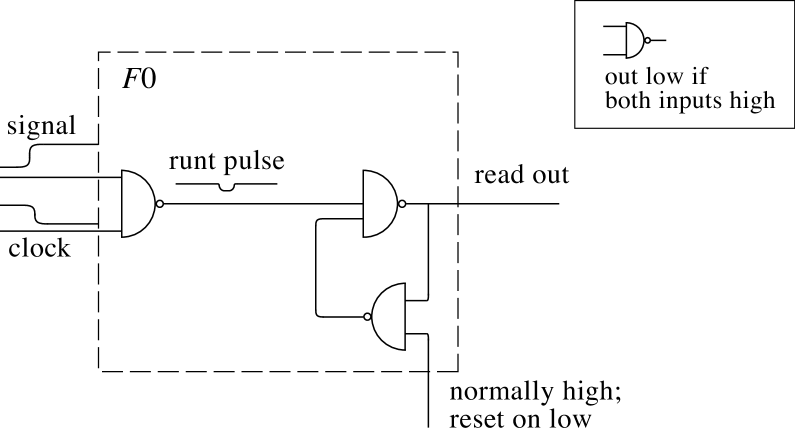
Figure 1: Flip-flop exposed to race between signal going high and clock going low.

We investigated a 1-bit recording device implemented in transistor-transistor logic circuitry as the flip-flop $F0$ shown in Fig. 1. In addition to power and ground leads not shown, the flip-flop has wire leads for input, clock, and read-out; it also has a lead that works as a reset knob when driven by a low voltage. The NAND gate into which both the clock and the signal feed acts as a switch. At each trial $F0$ is exposed to a race between a signal rising from low to high on the input line and the clock falling from high to low, which turns off the switch just as the signal is passing through it, resulting in a negative runt pulse emerging from the switch.

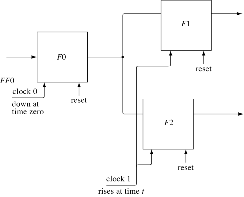
Figure 2: Flip-flops $F1$ and $F2$ used to read $F0$ after a delay $t$.

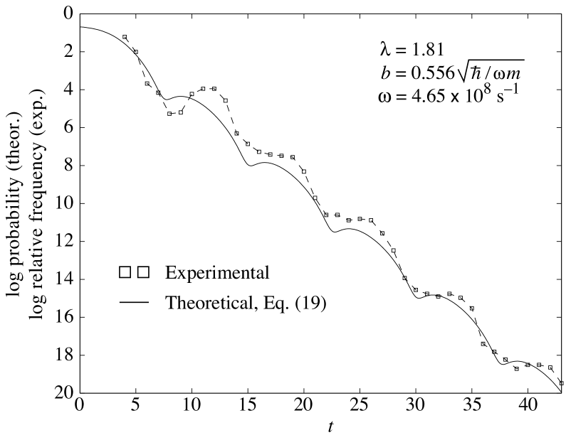
Figure 3: Probability of disagreement vs. settling time.

Besides the flip-flop $F0$ subjected to a race, two other flip-flops, $F1$ and $F2$ shown in Fig. 2, are used to record the result of each trial. The key experimental knob controls the delay time $t$ between exposing $F0$ to the race and a pulse on the clock-1 line that causes the reading of $F0$ by the paired flip-flops $F1$ and $F2$. After they read $F0$ and after an additional delay to assure that they have settled down, the bits recorded by $F1$ and $F2$ are tallied for later perusal. Figure 3 shows the experimental record of relative frequency of disagreement between $F1$ and $F2$ as a function of the waiting time $t$ between exposing $F0$ to the race and its reading by $F1$ and $F2$. While the flip-flops $F1$ and $F2$ and the other registers to which these transfer their results can be discussed in Turing language, the record displayed in Fig. 3 shows this is not the case for $F0$ exposed to a race condition.

V.3 Quantum-mechanical model of a metastable recording device

To model the metastable flip-flop $F0$ quantum-mechanically, notice that although recording devices are ordinarily assigned in models to the ‘detection’ side of the Heisenberg cut, there is no necessity for this, and in the present case, where $F0$ is part of what is being investigated, we can and do choose to model it as belonging to state preparation. In contrast, the flip-flops $F1$ and $F2$ that read $F0$ continue to be assigned to the detection side.

We invoke the rule of Sec. IV, according to which the modeling of whatever involves several detections must involve several particles. The flip-flop $F0$ is to be written into, and, before any later rewriting, it is to be read some number of times, say $n$ times. We model each reading as a detection, and hence are obliged by our rule to model the writing in the device as preparing at least $n$ particles, so that there can be $n$ detections.

Multiple readings entail the possibility of disagreements among them. Within the computer language of Turing tapes, any single reading can be expressed by a binary-valued variable $r\in\{0,1\}$. Allowing the possibility of disagreements, the expression of $n$ readings of 1 bit is then a bit string $\vec{r}=(r_{1},\dots,r_{n})\in\{0,1\}^{n}$. To connect this Turing language to the laboratory record, one has to partition the possible experimental outcomes into (at least) $2^{n}$ blocks and interpret these as corresponding one-to-one to the $2^{n}$ possible values of $\vec{r}$.

To model a 1-bit recording device, we focus not on experimental outcomes, but on outcomes in the mathematical sense of subsets of $\Omega$ to which probabilities are assigned by an equation of the form (3). Thus in our model $\alpha$ we will associate to each $\vec{r}$ a subset $\omega(\vec{r})\in\Omega$ with the notion that $\mu_{\alpha}(a,b)(\omega(\vec{r}))$ is the probability asserted by the model $\alpha$ for the outcome $\vec{r}$, given knob settings $a$ and $b$. With this in mind we propose a class of quantum-mechanical models of a 1-bit recording device, guided by the following considerations:

1. We model the recording of a bit—writing—as the preparation of a wave function satisfying a Schrödinger equation.

2. Writing of a bit that can be read some number $n$ times is modeled by the preparation of a $n$-particle wave function.

3. Each of the $2^{n}$ possible results of $n$ readings of 1 bit corresponds to one of $2^{n}$ mutually disjoint subsets of (the mathematical) outcome space $\Omega$. Of special interest are the two subsets $R_{0},R_{1}\subset\Omega$, interpreted as follows: the probability $\mu(R_{0})$ is taken to be the probability of an $n$-fold reading $r_{\ell}=0,\ell=1,\dots,n$, and similarly the probability $\mu(R_{1})$ is taken to be the probability of an $n$-fold reading $r_{\ell}=1,\ell=1,\dots,n$.

   1. The (unambiguous) writing of a 0 is modeled by the preparation of a $n$-particle wave function $\psi_{0}$ which evolves over time to produce a probability near 1 for an outcome in region $R_{0}$.

   2. The writing of a 1 is modeled by the preparation of a different wave function $\psi_{1}$ which evolves to produce a probability near 1 for detecting $n$ particles in region $R_{1}$.

4. We model a race condition as follows:

   1. Writing prepares an $n$-particle wave function intermediate between that for a 0 and that for a 1.

   2. Discrepancies of readings of the 1-bit device correspond to detections of $n$ particles in regions other than $R_{1}$ and $R_{0}$.

   3. An interaction term in the Schrödinger equation for the $n$-particle wave function couples the particles to produce a growth over time in correlation in the $n$-particle detection probability, meaning that the outcome regions other than $R_{0}$ and $R_{1}$ become progressively less likely.

Remark: The experimental records of the race condition do not accord with any model we know in which the wave function for the race condition is a quantum superposition of $\psi_{0}$ and $\psi_{1}$; thus the $\psi_{\mathrm{race}}$ is intermediate between $\psi_{0}$ and $\psi_{1}$ but is not a superposition of them.

For simplicity, we consider only a single space dimension for each of $n=2$ particles. Let $x$ be the space coordinate for one particle and $y$ be the space coordinate for the other particle (so $x$ and $y$ are coordinates for two particles moving in the same single space dimension, not for one particle with two space dimensions). The region $R_{0}$ is the region $x,y<0$, the region $R_{1}$ is the region $x,y>0$. Notice that this leaves two quadrants of the $(x,y)$-plane for discrepancies in which one reading yields a 0 while the other reading yields a 1. The model proposed will be analyzed to see what it says about the probability of discrepancies between paired detections, and how this probability varies over time.

We now specify the 2-particle Schrödinger equation which is the heart of this model. Characterizing a 1-bit recording device by an energy hump and assuming that what matters about this hump for long-time settling behavior is its curvature, we start by expressing uncoupled particles traveling in the presence of a parabolic energy hump. A single such particle, say the $x$-particle, is expressed by

$$i\hbar\,\frac{\partial\;}{\partial t}\,\psi(x,t)=\left(-\frac{\hbar^{2}}{2m}\,\frac{\partial^{2}\;}{\partial x^{2}}-\frac{kx^{2}}{2}\right)\psi(x,t).$$ (14)

Equation (14) is the quantum-mechanical equation for an unstable oscillator, the instability coming from the minus sign in the term proportional to $x^{2}$. To model a 1-bit recording device that can be read twice we augment this equation by adding a $y$-particle. The effect of the energy hump on this particle is then expressed by a term $-ky^{2}/2$ in the hamiltonian. In order to produce growth over time in the correlation of the detection probabilities, we put in the coupling term $\frac{1}{4}\lambda(x-y)^{2}$. This makes the following two-particle Schrödinger equation:

$$i\hbar\,\frac{\partial\;}{\partial t}\,\psi(x,y,t)=-\frac{\hbar^{2}}{2m}\left(\frac{\partial^{2}\;}{\partial x^{2}}+\frac{\partial^{2}\;}{\partial y^{2}}\right)\psi(x,y,t)+\frac{k}{2}\left(-x^{2}-y^{2}+\frac{\lambda}{2}(x-y)^{2}\right)\psi(x,y,t).$$ (15)

The natural time parameter for this equation is $\omega^{-1}$ defined here by $\omega\mathop{\stackrel{{\scriptstyle\mathrm{def}}}{{=}}}\nolimits\sqrt{k/m}$; similarly there is a natural distance parameter $\sqrt{\hbar/m\omega}$.

V.4 Initial conditions

For the initial condition, we will explore a wave packet of the form:

$$\psi(x,y,0)=\frac{1}{\pi^{1/2}b}\exp[-(x-c)^{2}/2b^{2}]\exp[(y-c)^{2}/2b^{2}].$$ (16)

For $c=0$, this puts the recording device exactly on edge, while positive or negative values of $c$ bias the recording device toward 1 or 0, respectively.

V.5 Solution

As discussed in Appendix A, the solution to this model is

$$|\psi(x,y,t)|^{2}=\frac{1}{\pi B_{1}(t)B_{2}(t)}\,\exp\left\{-\left(\frac{x+y}{\sqrt{2}}-c\sqrt{2}\cosh t\right)^{2}\Bigg{/}B^{2}(t)-\frac{(x-y)^{2}}{2B^{2}_{2}(t)}\right\},$$ (17)

with

$$B_{1}^{2}(t) \mskip-3.0mu=\mskip-3.0mu b^{2}\left[1+\left(\frac{\hbar^{2}}{\omega^{2}m^{2}b^{4}}+1\right)\sinh^{2}t\right]$$

$$B_{2}^{2}(t) \mskip-3.0mu=\mskip-3.0mu b^{2}\left[1+\left(\frac{\hbar^{2}}{\omega^{2}m^{2}b^{4}(\lambda-1)}-1\right)\sin^{2}\sqrt{\lambda-1}\,t\right].$$ (18)

The probability of two detections disagreeing is the integral of this density over the second and fourth quadrants of the $(x,y)$-plane. For the especially interesting case of $c=0$, this integral can be evaluated explicitly as shown in Appendix A:

$$\Pr(F1\text{ and }F2\text{ disagree at }t)=\frac{2}{\pi}\tan^{-1}\left(\frac{\displaystyle 1+\left[\frac{\hbar^{2}}{\omega^{2}m^{2}b^{4}(\lambda-1)}-1\right]\sin^{2}\sqrt{\lambda-1}\,\omega t}{\displaystyle 1+\left(\frac{\hbar^{2}}{\omega^{2}m^{2}b^{4}}+1\right)\sinh^{2}\omega t}\right)^{1/2}.$$ (19)

This formula works for all real $\lambda$. For $\lambda>1$, it shows an oscillation, as illustrated in Fig. 3. For the case $0<\lambda<1$, the numerator takes on the same form as the denominator, but with a slower growth with time and lacking the oscillation, so that the probability of disagreement still decreases with time, but more slowly. Picking values of $b$ and $\lambda$ to fit the experimental record, we get the theoretical curve of Fig. 3, shown in comparison with the relative frequencies (dashed curve) taken from the experimental record. For the curve shown, $\,\lambda=1.81$ and $b=0.556$ times the characteristic distance $\sqrt{\hbar/\omega m}$. According to this model $\alpha$, a design to decrease the half-life of disagreement calls for making both $k/m$ and $\lambda$ large. Raising $\lambda$ above 1 has the consequence of the oscillation, which can be stronger than that shown in Fig. 3. When the oscillation is pronounced, the probability of disagreement, while decreasing with the waiting time $t$, is not monotonic, so in some cases judging sooner has less risk of disagreement than judging later.

V.6 An alternative to model $\alpha$

Proposition 2 of Sec. III asserts that whenever one model works, so do other quite different models, and indeed we can construct alternatives to the above model $\alpha$ of a 1-bit recording device. Where model $\alpha$ distinguishes an initial condition for writing a 0 from that for writing a 1 by “placing a blob,” expressed in the choice of the value of $c$ in Eq. (16), a model $\beta$ can distinguish writing a 0 from writing a 1 by “shooting a particle at an energy hump” with less or more energy of wave functions initially concentrated in a region in which $x$ and $y$ are negative and propagating toward the energy saddle at $x,y=0$. Model $\beta$ can preserve the interpretation of detection probabilities (e.g., $\,x,y>0$ corresponds to both detectors reading a 1). Hints for this construction can be found in the paper of Barton barton , which contains a careful discussion of the energy eigenfunctions for the single inverted oscillator of Eq. (29), as well as of wave packets constructed from these eigenfunctions.

Such a model $\beta$ based on an energy distinction emphasizes the role of a 1-bit recording device as a decision device: it “decides” whether a signal is above or below the energy threshold. For this reason, energy-based models of a 1-bit recording device exposed to a race condition can be applied to detectors working at the threshold of detectability. It would be interesting to look for the behavior shown here for recording devices, including the oscillation, in a photodetector used to detect light at energies at or below a single-photon level.

V.7 The dependence of probability of disagreement on $\hbar$

For finite $b$, the limit of Eq. (19) as $\hbar\rightarrow 0$ is

$$\Pr(F1\text{ and }F2\text{ disagree at }t)=\frac{2}{\pi}\tan^{-1}\left(\left|\frac{\cos\sqrt{\lambda-1}\,\omega t}{\cosh\omega t}\right|\right).$$ (20)

This classical limit of model $\alpha$ contrasts with the quantum-mechanical Eq. (19) in how the disagreement probability depends on $\lambda$. Quantum behavior is also evident in entanglement exhibited by the quantum-mechanical model. At $t=0$ the wave function is the unentangled product state of Eq. (16). Although it remains in a product state when viewed in $(u,v)$-coordinates discussed in Appendix A, as a function of $(x,y)$-coordinates it becomes more and more entangled with time, as it must to exhibit correlations in detection probabilities for the $x$- and $y$-particles. By virtue of a time-growing entanglement and the stark contrast between Eq. (19) and its classical limit, the behavior of the 1-bit recording device exhibits quantum-mechanical effects significantly different from any classical description.

The alternative model $\beta$ based on energy differences can be expected to depend on a sojourn time with its interesting dependence on Planck’s constant, as discussed by Barton barton . Another variation in models, call it $\gamma$, would distinguish between 0 and 1 in terms of momenta rather than location; it too is expected to have a robust dependence on $\hbar$. These models thus bring Planck’s constant into the description of decision and recording devices, not by building up the devices atom by atom, so to speak, but by tying quantum mechanics directly to the experimentally recorded relative frequencies of outcomes of uses of the devices.

Appendix A Solution to Model $\alpha$ of a 1-bit recording device

Starting with Eq. (15), and writing $t$ as the time parameter times a dimensionless “$t$” and $x$ and $y$ as the distance parameter times dimensionless “$x$” and “$y$,” respectively, we obtain

$$i\,\frac{\partial\;}{\partial t}\,\psi(x,y,t)=\frac{1}{2}\left(-\frac{\partial^{2}\;}{\partial x^{2}}-\frac{\partial^{2}\;}{\partial y^{2}}-x^{2}-y^{2}+\frac{\lambda}{2}(x-y)^{2}\right)\psi(x,y,t).$$ (21)

This equation is solved by introducing a non-local coordinate change:

$$u=\frac{x+y}{\sqrt{2}}\quad\text{and}\quad v=\frac{x-y}{\sqrt{2}}.$$ (22)

With this change of variable, Eq. (21) becomes

$$i\,\frac{\partial\;}{\partial t}\,\psi(u,v,t)=\frac{1}{2}\left(-\frac{\partial^{2}\;}{\partial u^{2}}-\frac{\partial^{2}\;}{\partial v^{2}}-u^{2}+(\lambda-1)v^{2}\right)\psi(u,v,t),$$ (23)

for which separation of variables is immediate, so the general solution is a sum of products, each of the form

$$\psi(u,v,t)=\phi(u,t)\chi(v,t).$$ (24)

The function $\phi$ satisfies its own Schrödinger equation,

$$\left(i\,\frac{\partial\;}{\partial t}+\frac{1}{2}\,\frac{\partial^{2}\;}{\partial u^{2}}+\frac{u^{2}}{2}\right)\phi(u,t)=0,$$ (25)

which is the quantum-mechanical equation for an unstable harmonic oscillator, while $\chi$ satisfies

$$\left(i\,\frac{\partial\;}{\partial t}+\frac{1}{2}\,\frac{\partial^{2}\;}{\partial v^{2}}+\frac{1-\lambda}{2}\,v^{2}\right)\chi(v,t)=0,$$ (26)

which varies in its interpretation according to the value of $\lambda$, as follows: (a) for $\lambda<1$ it expresses an unstable harmonic oscillator; (b) for $\lambda=1$ it expresses a free particle, and (c) for $\lambda>1$ it expresses a stable harmonic oscillator. The last case will be of interest when we compare behavior of the model with an experimental record.

By translating Eq. (16) into $(u,v)$-coordinates, one obtains initial conditions

$$\phi(u,0) \mskip-3.0mu=\mskip-3.0mu \pi^{-1/4}b^{-1/2}\exp\left\{-\frac{(u-\sqrt{2}c)^{2}}{2b^{2}}\right\},$$ (27)

$$\chi(v,0) \mskip-3.0mu=\mskip-3.0mu \pi^{-1/4}b^{-1/2}\exp\left\{-\frac{v^{2}}{2b^{2}}\right\}.$$ (28)

The solution to Eq. (25) with these initial conditions is given by Barton barton ; we deal with $\phi$ and $\chi$ in order. From (5.3) of Ref. barton , one has

$$|\phi(u,t)|^{2}=\frac{1}{\pi^{1/2}B_{1}(t)}\exp\left\{\frac{-(u-c\sqrt{2}\cosh t)^{2}}{B_{1}^{2}(t)}\right\},$$ (29)

where

$$B_{1}^{2}(t)=b^{2}\left[1+\left(\frac{1}{b^{4}}+1\right)\sinh^{2}t\right].$$ (30)

Similarly, integrating the Green’s function for the stable oscillator ($\lambda>1)$ over the initial condition for $\chi$ yields

$$|\chi(v,t)|^{2}=\frac{1}{\pi^{1/2}B_{2}(t)}\exp\left\{\frac{-v^{2}}{B_{2}^{2}(t)}\right\},$$ (31)

where

$$B_{2}^{2}(t)=b^{2}\left[1+\left(\frac{1}{b^{4}(\lambda-1)}-1\right)\sin^{2}\sqrt{\lambda-1}\,t\right]$$ (32)

Multiplying these and changing back to $(x,y)$-coordinates yield the joint probability density

$$|\psi(x,y,t)|^{2}=\frac{1}{\pi B_{1}(t)B_{2}(t)}\,\exp\left\{-\left(\frac{x+y}{\sqrt{2}}-c\sqrt{2}\cosh t\right)^{2}\Bigg{/}B^{2}(t)-\frac{(x-y)^{2}}{2B^{2}_{2}(t)}\right\}.$$ (33)

The probability of two detections disagreeing is the integral of this density over the second and fourth quadrants of the $(x,y)$-plane. This is most conveniently carried out in $(u,v)$-coordinates. For the especially interesting case of $c=0$ (and $\lambda>1)$, this integral can be transformed into

$$\Pr(F1\text{ and }F2\text{ disagree at }t) \mskip-3.0mu=\mskip-3.0mu \frac{1}{\pi B_{1}(t)B_{2}(t)}\int^{\infty}_{-\infty}dv\int^{v}_{-v}du\,\exp\left\{\frac{-u^{2}}{B_{1}^{2}(t)}-\frac{v^{2}}{B_{2}^{2}(t)}\right\}$$ (34)

$$\mskip-3.0mu=\mskip-3.0mu \frac{4}{\pi}\int_{0}^{\infty}e^{-V^{2}}\,dV\int_{0}^{B_{2}(t)V/B_{1}(t)}dU\,e^{-U^{2}}$$

$$\mskip-3.0mu=\mskip-3.0mu \frac{2}{\pi}\tan^{-1}\left(\frac{B_{2}(t)}{B_{1}(t)}\right)$$

$$\mskip-3.0mu=\mskip-3.0mu \frac{2}{\pi}\tan^{-1}\left(\frac{\displaystyle 1+\left[\frac{1}{b^{4}(\lambda-1)}-1\right]\sin^{2}\sqrt{\lambda-1}\,t}{\displaystyle 1+\left(\frac{1}{b^{4}}+1\right)\sinh^{2}t}\right)^{1/2}.\qquad$$

It is easy to check that this formula works not only when $\lambda>1$ but also for the case $\lambda<1$. For $0<\lambda<1$, the numerator takes on the same form as the denominator, but with a slower growth with time, so that the probability of disagreement still decreases with time exponentially, but more slowly.

Converting Eq. (33) from dimensionless back to physical time and distance variables results in Eq. (17), and similarly Eq. (34) leads to Eq. (19).

Figure Captions

Figure 1: Flip-flop exposed to race between signal going high and clock going low.

Figure 2: Flip-flops $F1$ and $F2$ used to read $F0$ after a delay $t$.

Figure 3: Probability of disagreement vs. settling time.

References

- (1) H. J. Gray, Digital Computer Engineering (Prentice Hall, Englewood Cliffs, NJ, 1963), pp. 198–201.
- (2) T. J. Chaney and C. E. Molnar, IEEE Trans. Computers C-22, 421 (1973).
- (3) A. M. Turing, Proc. London Math. Society (2), 42, 230–265 (1936).
- (4) P. A. M. Dirac, The Principles of Quantum Mechanics, 4th ed. (Clarendon Press, Oxford, 1958).
- (5) J. Von Neumann, Mathematical Foundations of Quantum Mechanics (Princeton University Press, Princeton, 1955).
- (6) W. Rudin, Real and Complex Analysis, 3rd ed. (McGraw-Hill, New York, 1966).
- (7) W. Rudin, Functional Analysis, 2nd ed. (McGraw-Hill, New York, 1973).
- (8) J. M. Myers and F. H. Madjid, J. Opt. B: Quantum Semiclass. Opt. 4, S109–S116 (2002).
- (9) W. K. Wooters, Phys. Rev. D, 23, 357–362 (1981).
- (10) J. M. Myers and F. H. Madjid, “A proof that measured data and equations of quantum mechanics can be linked only by guesswork” in Quantum Computation and Information, S. J. Lomonaco, Jr. and H. E. Brandt, eds. (American Mathematical Society, Contemporary Mathematics Series. Vol. 305, 2002), pp. 221–244.
- (11) M. Born, Zeitschrift für Physik, 37 (1926).
- (12) F. H. Madjid and J. M. Myers, Annals of Physics (NY), 221, 258–305 (1993).
- (13) G. Barton, Annals of Physics (NY), 166, 322–263 (1986).