Spin-based all-optical quantum computation with quantum dots:
understanding and suppressing decoherence

Abstract

We present an all-optical implementation of quantum computation using semiconductor quantum dots. Quantum memory is represented by the spin of an excess electron stored in each dot. Two-qubit gates are realized by switching on trion-trion interactions between different dots. State selectivity is achieved via conditional laser excitation exploiting Pauli exclusion principle. Read-out is performed via a quantum-jump technique. We analyze the effect on our scheme’s performance of the main imperfections present in real quantum dots: exciton decay, hole mixing and phonon decoherence. We introduce an adiabatic gate procedure that allows one to circumvent these effects, and evaluate quantitatively its fidelity.

I Introduction

The promise of quantum computation is to enable algorithms which render feasible problems requiring exorbitant resources for their solution on a classical computer. This has stimulated a large number of proposals for the physical implementation of the elementary logical operations building up a general-purpose quantum computer FdP . A central issue is the trade-off between efficient coupling to the system, in order to control the quantized degrees of freedom, and good isolation from the environment, in order to preserve the coherence of the quantum evolution. Strategies have been developed to fight decoherence taking place during the computation, ranging from “active” (error-correcting) to “passive” (error-avoiding) schemes. Thereby, unwanted physical processes (i.e., computational errors) of a general kind can be compensated for, either by detecting and correcting their effect via redundant qubit encoding Error-correcting , or by decoupling the qubits from the environment dynamics through algebraic techniques exploiting symmetries in the evolution Error-avoiding . A less general, more implementation-dependent approach is to study the specific decoherence channels of a certain physical scheme, and to design gating processes that are stable against the relevant types of errors (for an example with ion traps, see Ref. ionPRA ).

In this paper, we adopt the latter point of view, and apply it to a recent proposal for all-optical quantum information processing based on charged semiconductor quantum dots pauli . In this scheme, quantum information is stored in the spin of an excess electron in a quantum dot (QD), and gating between 2 QDs is performed via optical excitation of electron-hole pairs (excitons), which in an external electric field acquire a dipole moment allowing them to interact with each other. In this way, the quantum memory coherence time is in the $\mu$s range, typical for spin degrees of freedom in semiconductor heterostructures spindeph , while the two-qubit gating time is in the ps range, as dictated by the electrostatic dipole-dipole interaction.

Decoherence is important mainly during gate operation when excitonic states are created that interact with the phonon bath. Recent calculations for the strong field limit kuhn indicate that the leading dephasing mechanism is the coupling to acoustic phonons. In this paper, we focus on this coupling mechanism, and we describe a procedure that allows one to circumvent, to a large extent, the limitations imposed by this decoherence channel on the fidelity $F$ of the gate operation. We will evaluate the dependence of $F$ on various parameters, including temperature, and take into account other sources of imperfection like heavy-/light-hole mixing.

We choose to neglect all kinds of nonidealities arising from limitations, e.g., in QD fabrication and manipulation techniques. We are well aware that these might yield the most significant problems for the implementation of our proposal in the immediate future. However, we prefer to focus on fundamental quantum-mechanical limitations of our physical system rather than on technical problems. Once the technological advances have overcome the latter, the relevant part will be to find ways to circumvent the former. The main purpose of this paper is to develop strategies aimed at this.

The paper is organized as follows: in Sec. II we describe the general idea of a two-qubit quantum gate based on selective switching of controlled interactions. In Sec. III we recall the dynamics of charge carriers in a quantum dot, including external static and oscillating electromagnetic fields. In Sec. IV we derive few-level model corresponding to the above general scheme and discuss some of its limitations. In Sec. V we discuss our two-qubit gate and develop its adiabatic version, suitable for operation even in realistic scenarios with hole mixing. In Sec. VI we propose a hole-mixing tolerant scheme for single-qubit operations. In Sec. VII we analyze the effect of the interaction with phonons on the performance of our adiabatic gates, showing that the gates indeed are quite robust also against this kind of imperfection. In Sec. VIII we describe how the quantum jump technique can be employed for measuring the spin state of a confined electron, emphasizing that this can be done even for the case of non-zero hole mixing. Our conclusions are summarized in Sec. IX.

II Quantum gate model

To execute an arbitrary quantum computation, i.e. to control the coherent evolution of a system composed of an arbitrary number of qubits, one does not need to realize physically arbitrary multi-qubit operations. On the contrary, just two kinds of elementary operations are sufficient, out of which all others can be constructed. These two elementary gates are the set of rotations of a single qubit, and a specific entangling operation on two qubits. Among the possible choices for the latter, one which is well suited for an implementation with atomic-like systems like quantum dots is the phase gate – a transformation which rotates by a certain phase just one component of logical states:

$$\begin{array}[]{rcrl}|0\rangle|0\rangle&\longrightarrow&|0\rangle|0\rangle&\\ |0\rangle|1\rangle&\longrightarrow&|0\rangle|1\rangle&\\ |1\rangle|0\rangle&\longrightarrow&|1\rangle|0\rangle&\\ |1\rangle|1\rangle&\longrightarrow&e^{i\vartheta}|1\rangle|1\rangle&\!\!\!.\end{array}$$ (1)

When we have $\vartheta=\pi$, this is equivalent, up to single-qubit rotations, to a controlled-NOT gate. Ideally, this would be accomplished by means of a state-dependent interaction of the form

$$H_{\mathrm{ideal}}=\Delta E_{ab}(t)\left|1\right\rangle_{a}\left\langle 1\right|\otimes\left|1\right\rangle_{b}\left\langle 1\right|.$$ (2)

This describes a situation in which the two-qubit system undergoes an energy shift $\Delta E_{ab}$ if and only if both qubits are in state $|1\rangle$. Imposing the additional condition

$$\int_{t_{0}}^{t_{0}+\tau}\Delta E_{ab}(t^{\prime})dt^{\prime}=\vartheta$$ (3)

on the time dependence of the energy shift, Eq. (1) is recovered.

II.1 Phase gate model: auxiliary interacting states

An interaction of the form Eq. (2) is not straightforwardly found in nature. Implementing it entails of course a certain degree of engineering “natural” interactions, i.e., those directly available in a specific physical system. This, together with other requirements on the stability of the available quantum memory, affects the choice of the particular qubit implementation. When it comes to systems of confined electrons in solid state systems, such as quantum dots, two different choices are natural for the logical degree of freedom: either charge excitation RossiPRL , or spin polarization LossDiVincenzo . The former provides for a strong interaction, leading to comparatively shorter gate times but to faster decoherence rates as well; conversely, the latter suffers less from the coupling to the environment, yielding better stability against memory decoherence, but bears also a weaker coupling between qubits, requiring longer times for gate operation. Aiming at a high ratio between coherence time and gate operation time leads to conflicting requirements. Reasonable trade-offs can be achieved in each case – however, sticking to the same degree of freedom for both the memory and the two-qubit interaction may be not necessarily the only option. For instance, the same effect of the interaction Eq. (2) can be obtained by introducing an auxiliary state $|x\rangle$. Let us consider two qubits, labeled by $a$ and $b$ and with logical states $|\alpha\rangle_{a,b}$ ($\alpha\in\{0,1\}$). Each qubit is selectively coupled to a further state $|x\rangle$ – namely, only $|1\rangle$ can be excited to $|x\rangle$. This situation is described by the following Hamiltonian:

$$H_{\mathrm{phys}}(t) = \!\sum_{\begin{subarray}{c}\alpha=0,1,x\\ \nu=a,b\end{subarray}}\!\!E_{\alpha}\left|\alpha\right\rangle_{\nu}\left\langle\alpha\right|+\frac{\Omega(t)}{2}\sum_{\nu=a,b}\left|x\right\rangle_{\nu}\left\langle 1\right|+\mathrm{h.c.}$$ (4)

$$\mbox{}+\Delta E_{ab}(t)\left|x\right\rangle_{a}\left\langle x\right|\otimes\left|x\right\rangle_{b}\left\langle x\right|$$

As in Ref. pauli , the logical states $|0\rangle$ and $|1\rangle$ (the quantum memory) can be encoded into long-coherence spin states, while the auxiliary states $|x\rangle$, needed for the gate to be performed, can be chosen to be electrostatically interacting states. State selectivity, required for conditional logical operations, is accomplished via the state-dependent coupling $\Omega(t)$. The simplest strategy for performing a quantum gate exploiting the coupling scheme Eq. (4) would be, e.g., to selectively excite the interacting state $|x\rangle$ via a Rabi flop, wait for the desired gate phase to be accumulated, and then de-excite. The interaction energy shift would then be effective only if both QDs started off state $|1\rangle$, as described in Fig. 1.

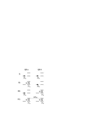
Figure 1: Gate operation via an auxiliary state: in the ideal scenario when only one of the logical states can be coupled to the interacting state, the interaction leading to the logical phase is “switched on” only when both qubits are in the same state (here, $|1\rangle$).

This procedure works in the ideal case when the coupling is perfectly state-selective as in Eq. (4). Compared to similar schemes for neutral atoms (see e.g. Rydberg ), it has also the advantage that quantum dots, unlike trapped atoms, are not subject to back-action on motional dynamics. However, in a real situation state selectivity may not be perfectly satisfied, in which case the simple procedure described above would not work. We will handle this imperfection below, and develop a strategy for overcoming it. But first we need a model of quantum dot dynamics that can account for Eq. (4). This is the subject of Sect. III.

II.2 Gate fidelity

To evaluate the performance of a quantum gate, one needs to compare its desired operation, Eq. (1) in our case, with the actual performance of the physical system which implements it. The fidelity $F$ represents a quantitative basis for this. To define it, let us start from the logical input state

$$\left|\chi\right\rangle\equiv c_{00}\left|00\right\rangle+c_{01}\left|01\right\rangle+c_{10}\left|10\right\rangle+c_{11}\left|11\right\rangle=\sum_{n=0}^{3}c_{n}\left|n\right\rangle,$$ (5)

which is an arbitrary superposition of all two-qubit computational basis states. The goal of gate operation is to obtain the ideal output

$$\left|\tilde{\chi}\right\rangle\equiv\sum_{n=0}^{3}e^{i\phi_{n}}c_{n}\left|n\right\rangle,$$ (6)

This is equivalent to the desired two-qubit transformation Eq. (1): one can be recovered from the other by redefining the logical states via single-qubit operations. The gate phase $\vartheta$ turns out to be related to the logical phases $\phi_{\alpha\beta}$ as follows ionPRA :

$$\vartheta=\phi_{00}-\phi_{01}-\phi_{10}+\phi_{11}.$$ (7)

Thus the condition $\vartheta\stackrel{{\scriptstyle!}}{{=}}\pi$ simply translates into a condition on the $\phi_{\alpha\beta}$’s.

The actual physical situation may involve other external (i.e., non-logical) degrees of freedom, which are not perfectly under control. In this case the initial state $\sigma$ will rather be a mixture:

$$\sigma\equiv\left|\chi\right\rangle\left\langle\chi\right|\otimes\rho_{\rm ext}(t_{0}),$$ (8)

where $\rho_{\rm ext}$ denotes the density matrix for external degrees of freedom. The operation $\cal U$ realized in the lab will in general involve both internal and external degrees of freedom in a non-trivial way: therefore the actual output

$$\sigma^{\prime}=\mathcal{U}\sigma\mathcal{U}^{\dagger}$$ (9)

will no longer be written in a simple factorized form like Eq. (8). In order to compare this state with the ideal one which would be obtained in the case of perfect operation, we define the fidelity

$$F=\min_{\chi}\mathrm{tr}_{\rm ext}\left\langle\tilde{\chi}\right|\sigma^{\prime}\left|\tilde{\chi}\right\rangle.$$ (10)

The intuitive meaning of this definition is that of a worst-case estimate (hence the minimum over the possible inputs $|\chi\rangle$) of the gate performance, averaged over the available non-logical states not being under control (hence the trace over the external degrees of freedom). Another option would be to define the fidelity as an average over the logical inputs $|\chi\rangle$ – however, we will stick to the minimum fidelity which gives a lower bound to the average fidelity.

Taking the most general possible form for the external state,

$$\rho_{ext}=\sum_{E}p_{E}\left|E\right\rangle\left\langle E\right|,$$ (11)

and assuming that the evolution does not mix different logical states,

$$\mathcal{U}\left|\chi\right\rangle\left|E\right\rangle\approx\sum_{n=0}^{3}c_{n}\left|n\right\rangle\otimes V_{n}\left|E\right\rangle,$$ (12)

the fidelity takes the form

$$F=\min_{\{c_{n}\}}\sum_{m,n=0}^{3}\left|c_{m}\right|^{2}\left|c_{n}\right|^{2}e^{i(\phi_{n}-\phi_{m})}\mathrm{tr}_{ext}\left(V_{m}V_{n}^{\dagger}\right),$$ (13)

which will be relevant for our calculations below.

III Quantum Dot dynamics

Quantum dots, due to their discrete density of states, are a very promising candidate for the implementation of quantum information processing RossiPRL ; Qdimplem . The brilliant idea first proposed by DiVincenzo and Loss LossDiVincenzo to employ the spin of an electron confined in a QD as the qubit degree of freedom has been developed by the authors over the years Lossrecent and is now pursued by many groups spinqu ; Imamoglu00 ; QED . Combining QD technology with ultra-fast laser pulses now seems to be one of the most promising channels for such an implementation scheme pauli ; spinoptic . Recently the necessary coherence required for such a task, i.e., Rabi oscillations, has been experimentally observed Rabi . There have been also impressive experimental achievements in exciting and probing excitons in QDs qdexciton .

The complex many-body dynamics of charge carriers in a semiconductor can be considerably simplified when considering semiconductor heterostructures like quantum wells and dots. The purpose of the present Section is to write down explicitly the carrier Hamiltonian for a quantum dot under these approximations. In the next Section this description will be linked to the particular model described by Eq. (4). Two main approximations Cardona ; Hawrylak are understood throughout the following. The first is the effective mass approximation, which arises from approximating the band dispersion relation around a band extremum up to second order in the carrier wavevector $k$. This is valid for small values of $k$, and allows for simplifying Hamiltonians in terms of effective electron and hole masses that take into account the underlying many-body dynamics. The other is the envelope function approximation Rossi , which is based on the following assumptions: (i) the different materials constituting the heterostructure are perfectly lattice-matched; (ii) the periodic parts of the Bloch functions $u_{l,\mathbf{0}}(\mathbf{r})$ are the same in the different layers; (iii) the confining potential is smoothly varying on the scale of the lattice structure, apart possibly from abrupt interfaces. The wavefunction can then be expanded as a sum of products of the rapidly varying functions $u_{l,\mathbf{0}}(\mathbf{r})$ by slowly varying envelope functions which obey an effective Schrödinger equation involving the effective masses. We consider QDs in the “strong-confinement” regime, in which the typical length scale in the growth direction $L$ is of the order of 10 nm to 20 nm. Considering QDs in the strong-confinement regime means that all relevant energy scales, e.g. charge carrier interactions in the QD or electron phonon interactions, will be small compared to the level spacing of the QD, typically of the order of $25$ meV for electrons.

III.1 Single-particle states under external fields

Under the above approximations, the carrier Hamiltonian for a quantum dot can be written as Hawrylak ; RossiPRB

$$H^{c}=H_{\perp}^{c}+H_{\parallel}^{c}=H_{\perp}^{e}+H_{\perp}^{h}+H_{\parallel}^{e}+H_{\parallel}^{h}$$ (14)

The electron in-plane Hamiltonian $H_{\parallel}^{e}$ describes the confinement in the direction perpendicular to the QD symmetry axis $\hat{z}$, which can be modeled with a parabolic potential:

$$H_{\parallel}^{e}=-\frac{\hbar^{2}}{2m_{e}}\nabla_{\mathbf{r}}^{2}+\frac{m_{e}\omega_{e}^{2}}{2}r^{2}+e\mathbf{F}\cdot\mathbf{r}$$ (15)

where the in-plane coordinate vector is $\mathbf{r}\equiv(x,y)$, and the electrical field $\mathbf{F}$ is taken to be parallel to the $xy$ plane. Defining

$$\mathbf{r}_{e}=\mathbf{r}+\frac{e\mathbf{F}}{m_{e}\omega_{e}^{2}}=(r_{e},\theta_{e}),$$ (16)

the eigenstates $\left|n,q\right\rangle^{e}$ of $H_{\parallel}^{e}$ in coordinate representation are

$$\left\langle r_{e}|n,q\right\rangle^{e}=\frac{r_{e}^{|q|}\sqrt{n_{r}!}e^{iq\theta_{e}-r_{e}^{2}/(2l_{0})^{2}}}{l_{0}^{|q|+1}\sqrt{\pi(n_{r}+|q|)!}}\mathcal{L}_{n_{r}}^{|q|}\left(\frac{r_{e}^{2}}{l_{0}^{2}}\right)$$ (17)

where $n=0,1,\ldots$ is the principal, $q=-n,-n+2,\ldots,n-2,n$ the azimuthal, and $n_{r}=(n-|q|)/2$ the radial quantum number; $\mathcal{L}_{n_{r}}^{|q|}\left(z\right)$ are Laguerre polynomials;

$$l_{0}=\sqrt{\frac{\hbar}{2m_{e}\omega_{0}}}$$ (18)

and the eigenenergies are

$$\epsilon_{nq}^{e}=\hbar(n+1)\omega_{0}.$$ (19)

In the growth direction the perpendicular Hamiltonian $H_{\perp}^{e}$ is in general a very narrow potential given by the quantum well structure and is therefore typically approximated by a step like potential. In the strong-confinement regime, a good approximation is to assume that the system remains in its ground state. Thus the problem effectively reduces to the in-plane dynamics. The hole Hamiltonian $H_{\perp,\parallel}^{h}$ is of course the same as $H_{\perp,\parallel}^{e}$ but with hole parameters $m_{h}$ and $\omega_{h}$, and opposite charge.

Due to the strong confinement and spatially symmetric shapes of the confining potentials in QDs, electronic angular momentum states can be defined. They exhibit many atomic-like symmetries which have been experimentally identified atomlike . In contrast to atoms, when considering the quantum numbers defining the angular momentum of an electron or a hole confined in a QDs, one has to take into account the underlying band structure Bastard .

Taking spin into account leads to splitting into hole subbands. The valence band, built from atomic $p$-type orbitals, contains states carrying an internal (band) angular momentum $\mathbf{m}$ equal to unity. Thus the total angular momentum is

$$\mathbf{j}=\mathbf{\sigma}+\mathbf{m}+\mathbf{l}$$ (20)

where $\mathbf{\sigma}$ is the spin and $\mathbf{l}$ the orbital angular momentum. Good quantum numbers are the modulus of $\mathbf{j}$ and its component along the QD symmetry axis $\hat{z}$. The single-particle states of the valence band with $\mathbf{l}=0$ are classified according to the value of $(|\mathbf{\sigma}+\mathbf{m}|,\sigma_{z}+m_{z})$, as follows:

$(3/2,\pm 3/2)$: heavy-hole subband;

$(3/2,\pm 1/2)$: light-hole subband;

$(1/2,\pm 1/2)$: spin-orbit split-off subband.

For the dynamics considered in this paper, only heavy and light holes will matter, the split-off subband being energetically far apart. So let us define electron and hole operators for the QD labeled by $\nu$ ($\nu\in\{a,b\}$), with composite index $i=[n,q]$ and spin $\sigma$:

$$c_{\nu,i,\sigma}^{\dagger}\left|\mathrm{vac}\right\rangle = \left|i,\sigma\right\rangle_{\nu},$$ (21)

$$h_{\nu,j,\sigma^{\prime}}^{\dagger}\left|\mathrm{vac}\right\rangle = \left|j,\sigma^{\prime}\right\rangle_{\nu}.$$ (22)

We can now write the noninteracting part of the carrier Hamiltonian for the QD $\nu$:

$$H_{\nu}^{c}=\sum_{i,\sigma=\pm 1/2}\epsilon_{i,\sigma}^{e}c_{\nu,i,\sigma}^{\dagger}c_{\nu,i,\sigma}+\sum_{j;\sigma^{\prime}=-3/2}^{3/2}\epsilon_{j,\sigma}^{h}h_{\nu,j,\sigma^{\prime}}^{\dagger}h_{\nu,j,\sigma^{\prime}}$$ (23)

III.2 Carrier-carrier interaction

The electrostatic interaction Hamiltonian is written as

$$H_{\nu}^{cc} = \sum_{\begin{subarray}{c}i,j,k,l\\ \sigma,\sigma^{\prime}\end{subarray}}\frac{1}{2}\left(\left\langle ij|V|kl\right\rangle_{ee}c_{\nu,i,\sigma}^{\dagger}c_{\nu,j,\sigma^{\prime}}^{\dagger}c_{\nu,l,\sigma}c_{\nu,k,\sigma^{\prime}}\right.$$

$$\left.+\left\langle ij|V|kl\right\rangle_{hh}h_{\nu,i,\sigma}^{\dagger}h_{\nu,j,\sigma^{\prime}}^{\dagger}h_{\nu,l,\sigma}h_{\nu,k,\sigma^{\prime}}\right)$$

$$-\left\langle ij|V|kl\right\rangle_{eh}c_{\nu,i,\sigma}^{\dagger}h_{\nu,j,\sigma^{\prime}}^{\dagger}c_{\nu,l,\sigma}h_{\nu,k,\sigma^{\prime}}$$

where the matrix elements of the Coulomb potential

$$V(\mathbf{r}-\mathbf{r}^{\prime})=\frac{e^{2}}{4\pi\epsilon\left|\mathbf{r}-\mathbf{r}^{\prime}\right|}$$ (25)

are calculated on electron and/or hole wavefunctions, according to subscripts. Here, carrier number conservation is assumed, since processes violating this (like e.g. Auger recombination and impact ionization) are relevant for energies and densities higher than we are considering RossiPRB . It should be noted that, in contrast to higher dimensional quantum structures, in QDs carrier-carrier interactions only induce an energy level renormalization without causing scattering or dephasing.

III.3 Interaction with a laser field

Let us consider a laser of amplitude $E(t)$ and central frequency $\omega_{L}$ impinging on our QD. Under the dipole and rotating-wave approximations dipoleapp the corresponding Hamiltonian is

$$H_{\nu}^{\mathrm{int}}=-\sum_{i,j,\sigma,\sigma^{\prime}}\left[\mu_{ij}^{\sigma\sigma^{\prime}}E^{\ast}(t)e^{-i\omega_{L}t}c_{\nu,i,\sigma}^{\dagger}h_{\nu,j,\sigma^{\prime}}^{\dagger}+\mathrm{h.c.}\right],$$ (26)

where $\mu_{ij}^{\sigma\sigma^{\prime}}$ is the dipole matrix element between the wave functions of an electron with spin $\sigma$ in state $i$ and a hole having angular momentum with $z$ component $\sigma^{\prime}$ in state $j$. The resulting selection rule is that the change in the number of electron-hole pairs can only be $\Delta N=\pm 1$.

IV Three-level model

Let us consider the QD identified by the index $\nu$, with an excess electron in the conduction-band ground state. We label its spin states with

$$\left|0\right\rangle_{\nu} \equiv c_{\nu,0,-1/2}^{\dagger}\left|\mathrm{vac}\right\rangle,$$ (27)

$$\left|1\right\rangle_{\nu} \equiv c_{\nu,0,1/2}^{\dagger}\left|\mathrm{vac}\right\rangle.$$ (28)

These are eigenstates of the bare Hamiltonian $H_{\nu}^{c}$, with eigenvalues $\epsilon^{e}_{0,-1/2}$ and $\epsilon^{e}_{0,1/2}$ respectively, and are not affected by the carrier-carrier interaction $H^{cc}_{\nu}$. On the other hand, in the so-called “trion” – i.e., the state obtained from Eqs.(27-28) by creating an exciton, having “bare” energy $\epsilon^{e}_{0,1/2}+\epsilon^{e}_{0,-1/2}+\epsilon^{h}_{0,\sigma_{h}}$ –, more than one carrier is present in the QD. Therefore, in this case the interaction $H^{cc}_{\nu}$ changes the bare state $c_{\nu,0,+1/2}^{\dagger}c_{\nu,0,-1/2}^{\dagger}h_{\nu,0,\sigma_{h}}^{\dagger}\left|\mathrm{vac}\right\rangle$ into the physical interacting state $\left|x,\sigma_{h}\right\rangle_{\nu}$, which we will take as our auxiliary state for gate operation. Such states were observed and studied experimentally in single self-assembled QDs trions .

According with the above selection rule, a laser pulse can excite at most one exciton. If the laser is tuned on the lowest interband excitation energy, then a ground-state exciton can be obtained. Due to angular momentum conservation, the hole angular momentum $\sigma_{h}$ will depend upon the laser polarization. For instance, in the case of a semiconductor material where heavy holes have the lowest energy, and assuming $\sigma^{+}$ circularly polarized light, the only hole state that can be excited has $\sigma_{h}=3/2$. If moreover the absolute value of the Rabi frequency, defined as

$$\Omega(t)\equiv\frac{2\mu_{00}^{-1/2,+3/2}E(t)}{\hbar},$$ (29)

is much smaller than the intraband excitation energy, $\left|\Omega\right|\ll\omega_{e,h}$, then we can neglect the probability of promoting the electron from the valence band to a higher-excited conduction band state. Under these assumptions, the interaction Hamiltonian Eq. (26) simplifies to

$$H_{\nu}^{\mathrm{int}}=\hbar\Omega(t)e^{-i\omega_{L}t}c_{\nu,0,-1/2}^{\dagger}h_{\nu,j,+3/2}^{\dagger}$$ (30)

If the temperature is sufficiently low with respect to the electronic intraband excitation energy, $k_{B}T\ll\hbar\omega_{e}$, then we can neglect also the excited states of the excess electron.

In the subspace defined by the states $\{\left|0\right\rangle_{\nu},\left|1\right\rangle_{\nu},\left|x,+3/2\right\rangle_{\nu}\}$, the effect of the carrier-carrier interaction term $H_{\nu}^{cc}$ will be to change the energy of the trion states. In particular, an external static electric field $\mathbf{F}$ applied in the $(x,y)$ plane will mutually displace the wavefunctions of the electron and of the hole which constitute an exciton, since they have opposite charge. In this way, the trion states acquire an electric dipole moment. The electrostatic interaction will then shift the energy of a trion state where a trion is also present in a neighboring dot. This energy difference, the so-called trion-trion shift $\Delta E_{ab}$, will be very important for obtaining the state-dependent phase needed for the logical gate to be performed. The key ingredient for this is a state-selective coupling of the logical states $\left|0\right\rangle$ and $\left|1\right\rangle$ to the auxiliary interacting state $\left|x^{\uparrow}\right\rangle\equiv\left|x,+3/2\right\rangle$. In the simplest, ideal case, this state-selectivity can be obtained if only one of the logical states is coupled to $\left|x^{\uparrow}\right\rangle$. The possibility of realizing physically such an effect in QDs is offered by the mechanism described in the following section.

IV.1 Exciton Pauli blocking

In fact, the Pauli exclusion principle forbids double occupancy of any of the electronic states. In particular, if the excess electron occupies the state $\left|0\right\rangle$, no further electron can be promoted from  the valence band into that state, and thus creation of an exciton by a $\sigma^{+}$-polarized laser pulse is inhibited (left part of Fig. 2). This effect, referred to as Pauli blocking, has been experimentally verified Warbuton97 . On the other hand, if the excess electron was in $\left|1\right\rangle$,  nothing could prevent a second electron from being excited to the state $\left|0\right\rangle$, thereby creating the trion state $\left|x^{\uparrow}\right\rangle$ (right part of Fig. 2) .

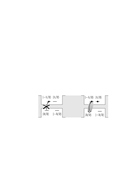
Figure 2: Pauli-blocking mechanism: a pulse of $\sigma_{+}$-polarized light can promote an electron from the valence band to the conduction-band $-1/2$-spin state of a quantum dot only if the latter is not occupied, i.e., if the excess electron in the dot is in the opposite spin state (right). Otherwise, no excitation takes place (left).

Taking now into account all of the above approximations and selection rules, we can write the following effective Hamiltonian for the dynamics of the relevant degrees of freedom in a frame rotating at the laser frequency $\omega_{L}$:

$$H_{\mathrm{eff}} = \hbar\sum_{\nu=a,b}\delta\left|1\right\rangle_{\nu}\left\langle 1\right|-\Delta(t)\left|x^{\uparrow}\right\rangle_{\nu}\left\langle x^{\uparrow}\right|$$

$$\mbox{}+\left[\frac{\Omega(t)}{2}\left|x^{\uparrow}\right\rangle_{\nu}\left\langle 1\right|+\mathrm{h.c.}\right]$$

$$\mbox{}+\Delta E_{ab}\left|x^{\uparrow}\right\rangle_{a}\left\langle x^{\uparrow}\right|\otimes\left|x^{\uparrow}\right\rangle_{b}\left\langle x^{\uparrow}\right|,$$

where for generality we have considered a chirped laser, i.e. one having a time-dependent detuning $\Delta(t)$ from the $\left|1\right\rangle\rightarrow\left|x^{\uparrow}\right\rangle$ transition. We have added a global (i.e., independent of the QD label) splitting $\delta$ between the two logical states, which can be realized, e.g., via an external static magnetic field. In the adiabatic scheme we are going to develop, this will have the effect of suppressing unwanted transitions between $|0\rangle$ and $|1\rangle$. This few state model will be valid for $\Omega$, $\Delta$, $\Delta E_{ab}/\hbar$, and the Fourier width of the pulse $\tau^{-1}$ to be much smaller than the QD level spacing, so that transitions to excited states are negligible. For $\Delta(t)=0$, $H_{\mathrm{eff}}$ has the same form as Eq. (4), and is thus suitable for quantum gate operation. A non-zero $\Delta(t)$ will turn out to be relevant for correcting the so-called hole-mixing problem, which is outlined in the following section.

IV.2 Hole mixing

Indeed, Eq. (IV.1) does not account for an important feature of a real QD system, namely the interaction between the hole subbands, described by the Luttinger Hamiltonian Luttinger . In this more accurate description, the actual hole eigenstates are no longer the ones described above. In  particular, the eigenstate of the (heavy) hole involved in the dynamics relevant to our study has to include a correction from the light-hole state $d_{\nu,0,+1/2}^{\dagger}\left|\mathrm{vac}\right\rangle$. Now, a pulse of $\sigma^{+}$-polarized light can promote an electron from the valence-band state corresponding to such light hole into the state $\left|1\right\rangle$. This means that the same laser we have included in the Hamiltonian Eq. (IV.1) has a certain probability amplitude to excite an exciton in the QD even if the initial excess electron state was $\left|0\right\rangle$, that is, the laser-coupling selection rules discussed above will be weakly violated in a real QD. This effect can be included in our simplified three-level model as an additional coupling between the states $\left|0\right\rangle$ and $\left|x^{\uparrow}\right\rangle$, induced by the laser with Rabi frequency $\Omega(t)$ and weighted by the effective parameter $\varepsilon$ whose typical value is at most 10%. This leads to the model Hamiltonian

$$H_{\mathrm{mix}} = \hbar\sum_{\nu=a,b}\delta\left|1\right\rangle_{\nu}\left\langle 1\right|-\Delta(t)\left|x^{\uparrow}\right\rangle_{\nu}\left\langle x^{\uparrow}\right|$$

$$\mbox{}+\left[\frac{\Omega(t)}{2}\left(\left|x^{\uparrow}\right\rangle_{\nu}\left\langle 1\right|+\varepsilon\left|x^{\uparrow}\right\rangle_{\nu}\left\langle 0\right|\right)+\mathrm{h.c.}\right]\qquad$$

$$\mbox{}+\Delta E_{ab}\left|x^{\uparrow}\right\rangle_{a}\left\langle x^{\uparrow}\right|\otimes\left|x^{\uparrow}\right\rangle_{b}\left\langle x^{\uparrow}\right|,$$

which will be the basis for our simulations.

V Two-qubit gate implementation

In this Section we show how the transformation Eq. (1) can be realized in practice using quantum dots. We will discuss the ideal scenario of perfect Pauli blocking as described in Eq. (IV.1), and then introduce imperfections. We will first lay out a strategy to overcome hole mixing, based on adiabatically chirped laser pulses. Then, in the next Section, we will show that the same strategy allows for suppressing the effect of phonon decoherence.

V.1 Ideal gate: $\varepsilon=0$

In the absence of hole mixing, the laser excitation of the trion is perfectly state-selective. In this ideal case, gate operation is particularly straightforward.

V.1.1 Direct Rabi excitation

The simplest quantum gate scheme exploiting the interaction Eq. (IV.1) is based on the following procedure:

1. selectively excite a trion via a resonant $\pi$ Rabi rotation;

2. wait a sufficient time $\tau\approx\pi\hbar/\Delta E_{ab}$ for the gate phase $\pi$ to be accumulated;

3. de-excite with a second $\pi$ pulse to return to the logical subspace.

This is depicted in Fig. 3.

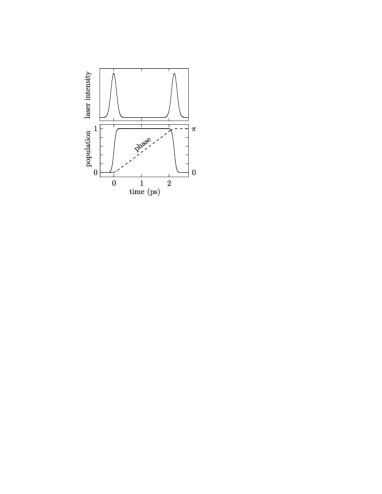
Figure 3: Two-qubit gate via direct Rabi excitation: pulse sequence for exciting and de-exciting the trion state in each dot (above); trion-trion population and accumulated interaction phase (below).

Since the trion-trion splitting can give an interaction time scale of the order of ps, such a gate would be pretty fast – however, unfortunately the scheme works only in the idealized model of perfect Pauli blocking. Therefore we want to develop an alternative excitation scheme, to be reliable also in the presence of hole mixing. This can be achieved by employing an adiabatic technique.

V.1.2 Adiabatic passage via dressed states

We want to design a process which allows to “switch on” the excitonic state for a certain time, and then to return to the initial ground state with the highest possible probability, by avoiding at the same time spontaneous emission. We can achieve this by using an adiabatically chirped laser pulse, i.e. one with a slowly changing detuning from the excitonic transition. Let us start by considering our driven two-level system

$$H_{0}=-\Delta\left|x\right\rangle\left\langle x\right|+\frac{\Omega}{2}\left|1\right\rangle\left\langle x\right|+h.c.$$ (33)

in the strong-coupling regime. Its two eigenstates (the so-called dressed states)

$$|+\rangle = \sin\frac{\theta}{2}|1\rangle+\cos\frac{\theta}{2}|x\rangle,$$ (34)

$$|-\rangle = \cos\frac{\theta}{2}|1\rangle-\sin\frac{\theta}{2}|x\rangle,$$ (35)

where

$$\tan\theta=-\Omega/\Delta\qquad(0\leq\theta\leq\pi),$$ (36)

have the energies

$$E_{\pm}=-\frac{\Delta}{2}\pm\frac{1}{2}\sqrt{\Delta^{2}+\Omega^{2}},$$ (37)

which are drawn in Fig. 4.

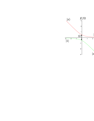
Figure 4: Dressed states in a driven two-level system.

Spontaneous emission can occur only if the system has a non vanishing probability amplitude of finding itself in its excited state. On the other hand, for small values of $\Delta/\Omega$ the dressed ground state contains a significant component of the interacting state $|x\rangle$. Hence, the following spontaneous-emission avoiding excitation procedure can be devised:

1. the system is prepared in the electronic ground state;

2. the laser excitation starts at a large negative value of $\Delta/\Omega$, where the lower dressed state tends to $|1\rangle$;

3. the laser parameters are slowly changed towards smaller values of $\Delta/\Omega$, achieving the transformation

   $$\alpha\left|0\right\rangle+\beta\left|1\right\rangle\rightarrow\alpha\left|0\right\rangle+\beta\left(\cos\frac{\theta}{2}\left|1\right\rangle-\sin\frac{\theta}{2}\left|x\right\rangle\right);$$ (38)

4. the system is adiabatically driven back to its initial state.

If such a chirped laser pulse is applied to two neighboring dots, they will still acquire a state-dependent trion-trion phase, due to the admixture from state $|x\rangle$ that is reached starting from state $|1\rangle$. The main constraint is that we want to change the Hamiltonian slowly enough such as to remain in the lower dressed state of the driven system with a high probability. We will show below that it is even possible to perform the operation in such a way that no phonon mode is excited during the gate, thus greatly reducing its sensitivity to temperature.

V.2 Hole-mixing-tolerant gate

In the presence of hole mixing, Pauli blocking does not work perfectly. Therefore a $2\pi$ pulse for the transition $|1\rangle\to|x^{\uparrow}\rangle$ will leave behind some excitonic population, causing decoherence. In this case only an adiabatic gate operation procedure can ensure that no excitonic population survive after gate operation. Let us therefore analyze it in more detail in the case when $\varepsilon\not=0$.

V.2.1 Hole-mixing-tolerant laser excitation

The Hamiltonian in this case is

$$H_{1}=H_{0}+\delta\left|1\right\rangle\left\langle 1\right|+\frac{\varepsilon\Omega}{2}\left|0\right\rangle\left\langle x\right|+h.c.$$ (39)

The level scheme for $H_{1}$ is drawn in Fig. 5. It shows an avoided crossing of the order of $\Omega$ between states $|1\rangle$ and $|x\rangle$ like in the two-level case, as well as a much smaller one between $|0\rangle$ and $|x\rangle$. However, the latter is found at more positive values of the detuning. Therefore, the same procedure as outlined above will work also in this case, while the adiabatic excitation Eq. (38) will be still approximately satisfied.

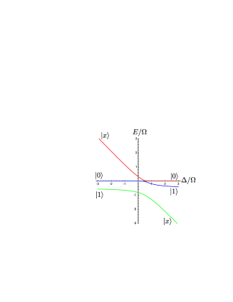
Figure 5: Dressed states in a driven three-level system. A typical hole mixing parameter value of $\varepsilon=0.1$ is assumed.

V.2.2 Two-qubit gate via chirped pulse

Let us now have a closer look to what happens when two neighboring dots undergo the above mentioned pulse sequence. The two-dot Hamiltonian, including trion-trion interaction, is

$$H_{2}=H_{1}^{a}+H_{1}^{b}+\Delta E_{ab}\left|x\right\rangle_{a}\left\langle x\right|\otimes\left|x\right\rangle_{b}\left\langle x\right|.$$ (40)

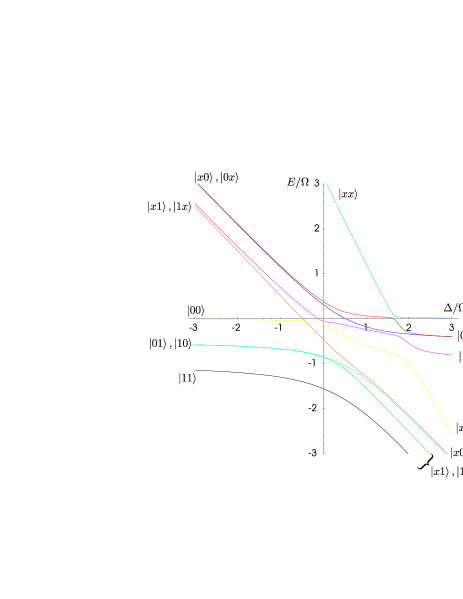
Figure 6: Level scheme of a system of two coupled quantum dots including hole mixing.

The level scheme is depicted in Fig. 6. Although it is of course significantly more complicated than the single-dot scheme of Fig. 5, the basic feature remains unchanged: under the same procedure as in the previous section, with the same laser pulse on both dots, different computational basis states will acquire different trion-trion amplitudes. This state selectivity allows one to obtain a nontrivial gate phase even in the presence of hole mixing, still avoiding spontaneous emission as discussed in Sec. V.1.2. We carried on a simulation using the following pulse shapes:

$$\Omega(t) = \Omega_{0}e^{-(t/\tau_{\Omega})^{2}},$$ (41)

$$\Delta(t) = \Delta_{\infty}\left[1-e^{-(t/\tau_{\Delta})^{2}}\right].$$ (42)

Results of the simulation with $\Delta E_{ab}=2$ meV, $\hbar\Delta_{\infty}=3$ meV, $\tau_{\Omega}=10$ ps, $\tau_{\Delta}=8.72$ ps, $\delta=0.5$ meV and $\hbar\Omega_{0}=3$ meV, are reported in Fig. 7. The gate phase $\vartheta=\pi$ is obtained in a longer time than in the simple Rabi-flopping scheme (Sec. V.1.1), since the procedure now has to be adiabatic to avoid excitations to decaying states. Indeed, the population left in the unwanted excitonic states remains below $10^{-6}$.

Figure 7: Hole-mixing-tolerant two-qubit gate operation via a chirped laser pulse: pulse shapes (above); interaction phase and trion-trion populations (below). The dashed line depicts the population in the $|xx\rangle$ state obtained starting from $|11\rangle$; the flat solid line the ones obtained starting from $|00\rangle$, $|01\rangle$ or $|10\rangle$.

VI Single-qubit operations

Contrary to atomic QC implementation schemes, implementing the single-qubit gate employing the spin state of an electron in a QD is of greater difficulty than implementing the two-qubit gate DiVincenzoNature . A natural candidate for an optical implementation of the spin rotation would be employing a two-photon Raman process involving an intermediate hole state. However, such a scheme is not possible since the lowest lying (long lived) hole states have $M_{J}^{h}=\pm 3/2$ symmetry, and there is, however, no strong dipole allowed two-photon coupling connecting the qubit states. This problem can be overcome by applying a transverse magnetic field, mixing the spin states and addressing the Zeeman split states in a frequency selective way, which however severely limits the Rabi frequencies and thus the gating time Imamoglu00 . An alternative is to make a Raman process via the lowest light hole states $M_{J}^{h}=\pm 1/2$ which however, being excited hole states, suffer from significant decoherence.

Employing II-VI semiconductors grown QDs avoids the above mentioned decoherence problems, since in these QDs the strain can shift the energy of the light holes to become the energetically lowest hole states light2 . Exploiting such QDs the single-qubit gate can be performed by the following pulse sequence: (i) a linearly polarized laser pulse couples the light-hole subband and the bottom of the conduction band (see Fig. 8).

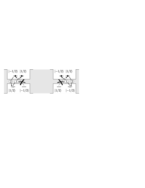
Figure 8: Single-qubit operation.

This linearly polarized pulse, which can be described as an equal-weighted superposition of $\sigma_{+}$ and $\sigma_{-}$ polarized light, attempts to create a trion-trion state in which both ground state electronic spin states are occupied but due to Pauli principle, a $\pi$-pulse of such a light will promote an electron only into the unoccupied qubit state – processes (1) in Fig. 8. (ii) A further $\pi$-pulse of $\sigma^{+}$ light now recombines the hole state with the original excess electron Fig. 8. In order to perform this recombination, i.e., changing the total angular momentum $\mathbf{j}$ by one unit and keeping its component along the QD symmetry axis $\hat{z}$ fixed, the laser pulse is shined in in-plane direction. This is achieved by employing a wave guide based scheme Weiner85 . The Hamiltonian describing the above process is given by:

$$H_{\rm 1q} = \hbar\frac{\Omega_{1}(t)}{2}\left(|{x_{l}}^{\downarrow}\rangle\langle 0|+\varepsilon|{x_{l}}^{\uparrow}\rangle\langle 0|\right.$$

$$\mbox{}+\left.|{x_{l}}^{\uparrow}\rangle\langle 1|+\varepsilon|{x_{l}}^{\downarrow}\rangle\langle 1|+{\rm h.c.}\right)$$

$$\mbox{}+\hbar\frac{\Omega_{2}(t)}{2}\left(|{x_{l}}^{\uparrow}\rangle\langle 0|+|{x_{l}}^{\downarrow}\rangle\langle 1|+{\rm h.c.}\right){}$$

$$\mbox{}-\Delta(t)\left(|{x_{l}}^{\downarrow}\rangle\langle{x_{l}}^{\downarrow}|+|{x_{l}}^{\uparrow}\rangle\langle{x_{l}}^{\uparrow}|\right)\ ,$$

where $\left|{x_{l}}^{\uparrow}\right\rangle\equiv\left|{x_{l}},+1/2\right\rangle,\left|{x_{l}}^{\downarrow}\right\rangle\equiv\left|{x_{l}},-1/2\right\rangle$ the $l$ index notation is used to indicate that the excitonic states are defined in terms of light holes, rather than of heavy holes as before. The electron-electron interaction appearing in the intermediate state has been absorbed by redefining the detuning. One should note that the heavy-light hole mixing has an effect only for the laser pulse directed in the growth direction, $\hat{z}$, the in-plane directed laser pulse does not induce transitions for the heavy hole part of the mixed wave function due to symmetry considerations. By properly adjusting the duration and the phase of the laser pulses, i.e., adiabatically eliminating the excitonic states, the following effective Hamiltonian is obtained:

$$H_{\rm 1q}^{eff}=\hbar\frac{\Omega_{eff}(t)}{2}\left|1\rangle\langle 0\right|+{\rm h.c.},$$ (43)

where $\Omega_{eff}=\sqrt{(\Omega_{1}\Omega_{2}+\varepsilon\Omega_{1}^{2})/\Delta}$ is the effective Rabi frequency for the coherent rotation between the two logical states. Thus utilizing strain inverted heavy-light hole II-VI semiconductors grown material, on which the adiabatic two qubit gate procedure can be adopted, single qubit optical gating can be induced on a pico-second time scale.

VII Phonons as a source of decoherence

VII.1 Interaction of quantum dots with phonons

The fidelity of the proposed qubit turns out to be quite good, and is determined by several mechanisms. Since the expected result is quite small, we can consider different sources of infidelity separately.

Due to the potentials confining electrons in all spatial dimensions which lead to a discrete density of states QDs are often referred to as “artificial atoms”. The major difference with respect to atoms is the coupling of the electrons to underlying lattice degrees of freedom, which lead to relatively faster decoherence times, on the order of tens of picoseconds excitondeph . In what follows we are developing a simple model of a QD interacting with a thermal bath of phonons.

In a large system of volume $V$ the displacement field is linear in creation and annihilation operators of phonons, $b_{j\mathbf{q}}$ and $b_{j\mathbf{q}}^{\dagger}$ respectively. Every phonon mode is characterized by its polarization $j$, momentum $\mathbf{q}$ and frequency $\omega_{j}(\mathbf{q})$. The number of phonon degrees of freedom is limited by the total number of atoms forming the lattice. Hence, there is a maximum frequency, usually defined via Debye temperature $\Theta$, so that $\omega_{j}(\mathbf{q})\lesssim\Theta$ (hereafter we use units such that $\hbar=k_{B}=1$). Normally $\Theta$ is very high (hundreds of K).

The minimal model describing the interaction of a charged quantum dot with the phonon field is given by the following Hamiltonian:

$$H_{\rm ph}=H_{\rm QD}-\mathbf{M}_{0}\mathbf{E}(c^{\dagger}h^{\dagger}+hc)+\sum_{j,\mathbf{q}}\omega_{j}(\mathbf{q})b_{j\mathbf{q}}^{\dagger}b_{j\mathbf{q}}+V_{int}.$$ (44)

The quantum dot is assumed to be in a time-dependent laser field $\mathbf{E}$. $\mathbf{M}_{0}$ is the dipole moment, and the Hamiltonian of an isolated QD is given by

$$H_{\rm QD}=\epsilon^{e}c^{\dagger}c+\epsilon^{h}h^{\dagger}h,$$ (45)

where $c$ and $h$ are the operators annihilating a ground-state electron and hole, respectively. Their spin dependence is not relevant here and will not be considered in what follows. As above, the quantities $\epsilon^{e}$ and $\epsilon^{h}$ are the energies of the single particle electron and hole states, respectively. The phonon coupling Hamiltonian is

$$V_{int}=\sum_{j,\mathbf{q}}\left[(g_{j\mathbf{q}}^{e}c^{\dagger}c-g_{j\mathbf{q}}^{h}h^{\dagger}h)b_{j\mathbf{q}}+c.c.\right],$$ (46)

where $g_{j\mathbf{q}}^{h}$ and $g_{j\mathbf{q}}^{e}$ are the coupling constants. The dynamics only couples the states $|g\rangle=|{\rm vac}\rangle$ and $|e\rangle=c^{\dagger}h^{\dagger}|{\rm vac}\rangle$. The matrix elements in this basis are: $\langle e|c^{\dagger}c|e\rangle=\langle e|h^{\dagger}h|e\rangle=1$ and $\langle e|c^{\dagger}h^{\dagger}|g\rangle=\langle g|ch|e\rangle=1$. These states are basically the logical and auxiliary states of the three-level model discussed in Sect. IV without the excess electron, namely, $|0\rangle=c_{0,-1/2}^{\dagger}|g\rangle$, $|1\rangle=c_{0,1/2}^{\dagger}|g\rangle$, and $|x,\sigma\rangle=c_{0,\sigma}^{\dagger}|e\rangle$.

Rewriting the laser field in the form: $E=E(t)\cos(\omega_{0}t)$, where $\omega_{0}$ is the laser frequency and $E(t)$ is the slow envelope, in the rotating wave approximation we obtain:

$$H_{\rm ph} = \Bigl{[}-\Delta+\sum_{j\mathbf{q}}\lambda_{j\mathbf{q}}(b_{j\mathbf{q}}+b_{j\mathbf{q}}^{\dagger})\Bigr{]}|e\rangle\langle e|$$ (47)

$$+\frac{\Omega}{2}(|e\rangle\langle g|+|g\rangle\langle e|)+\sum_{j,\mathbf{q}}\omega_{j}(\mathbf{q})b_{j\mathbf{q}}^{\dagger}b_{j\mathbf{q}},$$

where $\Delta$ is the laser frequency detuning, $\Omega=|\mathbf{M}_{0}\mathbf{E}(t)|$ is the Rabi frequency, and the phonon coupling strength is given by $\lambda_{j\mathbf{q}}=g_{j\mathbf{q}}^{e}-g_{j\mathbf{q}}^{h}$. This is identical, apart from the cavity terms, to the Imamoğlu–Wilson-Rae Hamiltonian WilsonRae (also used in Ref. kuhn ).

As we shall see, for slow processes considered below the interaction of a quantum dot with optical phonons is practically irrelevant. Indeed, optical phonons have a gap: $\omega_{opt}(\mathbf{q})\rightarrow\omega_{opt}\neq 0$ at $q\rightarrow 0$, which is large and hence optical phonons can always be adiabatically eliminated from the low frequency dynamics of the quantum dot. If taken into account, optical phonons contribution only renormalizes some quantities in the Hamiltonian (47). This is of course not really important for us, since we consider all the constants in the Hamiltonian as being phenomenological (essentially taken from experimental data). On the contrary, longitudinal acoustic phonons (LA phonons) have no gap: $\omega(\mathbf{q})=uq$ at $q\rightarrow 0$ ($u$ is the velocity of sound) and can effectively interact with low-frequency degrees of freedom of the Hamiltonian (47). Hereafter we will only consider LA phonons and omit the index $j$ everywhere.

The Hamiltonian (47) formally coincides with the Hamiltonian of the dissipative spin-boson model. The latter describes the interaction of a two-level system (spin) with the bath of harmonic oscillators (bosons). As described in Leggett , the important properties of the interaction of the quantum dot with the phonons are contained in the integrated quantity

$$J(\omega)=\sum_{\mathbf{q}}\lambda_{\mathbf{q}}^{2}\delta[\omega-\omega(\mathbf{q})].$$ (48)

One of the most important properties of the spectral function $J$ is its frequency dependence at small $\omega$: $J(\omega)\sim\omega^{s}$. The different values of the exponent $s$ distinguish between the cases of ohmic ($s=1$), sub- ($s<1$) and superohmic ($s>1$) couplings.

The phonons are coupled to the charge distribution in a quantum dot by means of either deformation or piezoelectric coupling potentials. The calculation of the spectral function $J$ requires a specific microscopic model. In the simplest case of a quantum dot characterized by a harmonic confinement potential the calculation is pretty easy, even if the QD is placed in external electric field (see Appendix A). The results of the calculation can be summarized as follows: both in the case of deformation and piezoelectric coupling the spectral function is superohmic, with $s=3$ and $s=5$, respectively. In both of the cases the spectral function can be approximately written as

$$J(\omega)\sim\omega^{s}\exp(-\omega^{2}/\omega_{l}^{2})$$ (49)

with a cut-off at $\omega_{l}\sim u/l$, where $l$ is the size of the quantum dot. This frequency is nothing else but the inverse phonon flight time through the quantum dot. The electric field (of reasonable intensity) does not change the exponent $s$ of the spectral function.

VII.2 Adiabatic Hamiltonian: Dressed states

Instead of considering the “bare” states $|e\rangle$ and $|g\rangle$ it is convenient to switch to the “adiabatic basis”: let us diagonalize first the quantum dot part of the Hamiltonian (47). The eigenstates (in terms of the bare states $|1\rangle$ and $|x\rangle$, which in the present discussion are replaced by $|g\rangle$ and $|e\rangle$, respectively) and energies are given in Sec. V.1.2.

The full interacting Hamiltonian (47) can be rewritten in the new basis and split into two parts: $H_{\rm ph}=H_{d}+H^{\prime}$, where

$$H_{d} = \Bigl{[}E_{+}+\sum_{\bf q}\omega({\bf q})b_{\bf q}^{\dagger}b_{\bf q}+\cos^{2}\frac{\theta}{2}\lambda_{\bf q}(b_{\bf q}^{\dagger}+b_{\bf q})\Bigr{]}|+\rangle\langle+|$$

$$+ \Bigl{[}E_{-}+\sum_{\bf q}\omega({\bf q})b_{\bf q}^{\dagger}b_{\bf q}-\sin^{2}\frac{\theta}{2}\lambda_{\bf q}(b_{\bf q}^{\dagger}+b_{\bf q})\Bigr{]}|-\rangle\langle-|,$$

and

$$H^{\prime}=-\frac{\sin\theta}{2}\sum_{\bf q}\lambda_{\bf q}(b_{\bf q}^{\dagger}+b_{\bf q})(|+\rangle\langle-|+|-\rangle\langle+|),$$ (51)

where $\tan(\theta)=-\Omega/\Delta$ so that $\theta$ is a time dependent quantity. The roles of the two Hamiltonians $H_{d}$ and $H^{\prime}$ are very different and will be considered separately below.

The interaction with the phonons can be understood in two ways. One of the remarkable non-perturbative simplifications can be used due to the fact that we are only dealing with the superohmic coupling case. For a slow process (the Hamiltonian parameters change on a time scale $\tau\omega_{l}\gg 1$) there is a way to adiabatically eliminate most of the “fast” phonon degrees of freedom with $\omega_{*}\lesssim\omega({\bf q})\ll\omega_{l}$ without relying on the pertubation expansion in phonon couplings $\lambda_{k}$. The resulting effective Hamiltonian has the same form as Eqs. (LABEL:eq:Hdiag-51), but with the summation restricted only to the phonon modes with $\omega({\bf q})\lesssim\omega_{*}$ and renormalized values of the Rabi frequency $\tilde{\Omega}$ and the detuning $\tilde{\Delta}$ (see the Appendix B). In what follows we will use both representations on the same footing and make no distinction between the bare and the renormalized quantities whenever it is not relevant.

VII.3 Diagonal and off-diagonal channels; Landau-Zener theory

Our qubit proposal relies on the fact, that the quantum dot stays in the same adiabatic ”dressed” state (34),(35) under slow variations of external parameters ($\Omega$ or $\Delta$). Therefore, transition between the adiabatic states (37) are a source of infidelity. Realistically every gate operation is performed with a finite speed and thus undesired transitions between the dressed states are always possible. In the absence of phonons the transition probability is given by the Landau-Zener theory. In its simplest version, i.e. for a case of linear detuning sweep $\Delta=\dot{\Delta}t$ around the resonance value $\Delta=0$, the measure of infidelity is given by the probability LL

$$P_{\pm}=\exp(-\pi\Omega^{2}/4\dot{\Delta}).$$ (52)

By requesting this quantity to be small we establish our adiabatic condition

$$\eta=\frac{\Omega^{2}}{\dot{\Delta}}\gg 1.$$ (53)

The condition has a simple physical meaning: the resonance is observed approximately when we have $\Delta\sim\Omega$, so $\tau\sim\Omega/\dot{\Delta}$ is nothing else but the characteristic time of the detuning sweep. Then, the adiabatic condition naturally implies that we have $\Omega\tau\gg 1$.

The effects of the interaction with phonons on this decoherence channel do not change this result much. As discussed in the Appendix B, both in the case of perturbation theory and in the adiabatic approximation the phonon interaction only renormalizes the Rabi frequency [see Eq. (105)]. Therefore, the same expression (52), but with the renormalized value of $\tilde{\Omega}$ instead of $\Omega$, holds even if the phonon coupling is strong.

Now let us consider the interaction with the phonons in some more detail. The phonon-assisted transitions between the dressed states $|\pm\rangle$ are possible and are described by the Hamiltonian (51). Since most of the transitions occurs close to the resonance $\Delta=0$, when the characteristic energy difference between the adiabatic levels is $\sim\Omega$, and the inter-level transition probability can be estimated using the Hamiltonian $H^{\prime}$ and the Fermi Golden Rule

$$P_{\pm}\sim\int_{\sim\Omega}^{\infty}|T_{\pm}(\omega)|^{2}J(\omega-\Omega)d\omega,$$ (54)

where

$$T_{\pm}(\omega)=\frac{1}{2}\int dt\exp(i\omega t)\sin[\theta(t)]$$ (55)

is the Fourier component of the “coupling potential” in Eq. (51). The latter can be easily estimated in the adiabatic limit by using the linear approximation for the detuning close to the resonance point (as above):

$$T_{\pm}(\omega)\sim\frac{\exp(-\omega/\omega_{m})}{(\omega\omega_{m})^{1/2}}$$ (56)

where we have $\omega_{m}=\tau^{-1}=\dot{\Delta}/\Omega$, and $\omega\gg\omega_{m}$. The frequency $\omega_{m}$ is the high-frequency cutoff imposed by the speed of the frequency detuning sweep. Substituting the above expression into Eq. (54) and integrating over $\omega$, we find the following estimation for the interstate transition probability:

$$P_{\pm}\sim\frac{J(\omega_{m})}{\Omega}\exp(-\alpha\Omega^{2}/\dot{\Delta}),$$ (57)

where $\alpha\sim 1$ is a numerical factor. This quantity characterizes the probability of unwanted processes and hence is a measure of infidelity. The result is exponentially small if we have $\omega_{m}\ll\Omega$, which is nothing else but our adiabaticity condition (53).

At finite temperatures there is an additional mechanism for decoherence: a quantum dot can interact with the phonon field and absorb a thermal phonon. Accordingly, the quantum dot acquires energy and is transformed into the excited dressed state. Nevertheless, the process can be easily suppressed by operating in the regime of small temperatures $T\ll\Omega$. In this case the transition probability is characterized by an additional small factor $\exp(-\Omega/T)\ll 1$ and can be disregarded.

Both probabilities (52) and (57) have similar structure and are exponentially small for adiabatic processes (53). In later sections we will find that the “diagonal” terms $H_{d}$ in the quantum dot Hamiltonian, though not changing the adiabatic states of the quantum dot, lead nevertheless to excitations of acoustical phonons and thus to a certain infidelity. The results do not contain exponentially small factors and hence the off-diagonal terms in the Hamiltonian considered here can be neglected in our further fidelity calculations.

VII.4 General expression for the fidelity in the presence of phonons

The major source of infidelity is the excitation of acoustical phonons without change of the quantum dot state, i.e., pure dephasing. To develop a formal approach to the fidelity calculation, we consider the evolution of a quantum dot coupled to a heat bath of phonons. Assume that at $t=-\infty$ the system starts from the state which is a direct product of pure quantum dot state and a thermal state of phonon field at a temperature $T$. As discussed in the previous section, the dynamics of the quantum dot can be well described (up to a few exponentially small amplitudes) by the diagonal Hamiltonian (LABEL:eq:Hdiag). Using this simplification, we can rewrite the density matrix of the quantum dot subsystem at $t=\infty$ as

$$\rho_{\alpha\beta}=\langle U_{\alpha}^{\dagger}\overleftarrow{T}\overrightarrow{T}U_{\beta}\rangle|\alpha\rangle\langle\beta|,$$ (58)

where $|\alpha\rangle$ is the quantum dot state, $\langle...\rangle$ is the average over the initial phonon state, $\overrightarrow{T}$ is the time ordering sign, and the (diagonal in the dressed state basis) evolution operators are given by

$$\overrightarrow{T}U_{\alpha}=\overrightarrow{T}\exp\Bigl{\{}-i\int dt\Bigl{[}f_{\alpha}(t)\sum_{k}\lambda_{k}(b_{k}+b_{k}^{\dagger})+E_{\alpha}\Bigr{]}\Bigr{\}},$$ (59)

with $f_{+}=\cos^{2}(\theta(t)/2)$ and $f_{-}=-\sin^{2}(\theta(t)/2)$. The time ordering is not convenient and can be removed by transforming the evolution operator into

$$\overrightarrow{T}U_{\alpha}=\exp\Bigl{\{}-i\int_{-\infty}^{\infty}dt\Bigl{[}f_{\alpha}(t)\sum_{k}\lambda_{k}(b_{k}+b_{k}^{\dagger})+E_{\alpha}\Bigr{]}+i\phi_{\alpha}\Bigr{\}},$$ (60)

where

$$\phi_{\alpha}=\int_{-\infty}^{\infty}dt\int_{\infty}^{t}dt^{\prime}f_{\alpha}(t)f_{\alpha}(t^{\prime})\sum_{k}\lambda_{k}^{2}\sin\omega_{k}(t-t^{\prime})$$ (61)

is the phase originating from the non-commutativity of $b_{k}$ operators at different times. Combining these results together we obtain the following expression for the fidelity matrix $T_{\alpha\beta}=\langle U_{\alpha}^{\dagger}\overleftarrow{T}\overrightarrow{T}U_{\beta}\rangle$:

$$T_{\alpha\beta}=\Bigl{\langle}\exp\Bigl{\{}-i\int_{-\infty}^{\infty}dta_{\alpha\beta}(t)\sum_{k}\lambda_{k}(b_{k}+b_{k}^{\dagger})+i\phi_{\alpha\beta}\Bigr{\}}\Bigr{\rangle},$$ (62)

where $a_{\alpha\beta}=f_{\alpha}-f_{\beta}$, and

$$\phi_{\alpha\beta} = \phi_{\beta}-\phi_{\alpha}+\int_{-\infty}^{\infty}dt\left[E_{\beta}(t)-E_{\alpha}(t)\right]$$

$$+\iint dtdt^{\prime}f_{\alpha}(t)f_{\beta}(t^{\prime})\sum_{k}\lambda_{k}^{2}\sin\omega_{k}(t-t^{\prime}).$$

The fidelity matrix $T$ can be used to rewrite Eq. (58) in a more convenient form. Consider an arbitrary pure state of a quantum dot $\Psi=\sum_{\alpha}c_{\alpha}|\alpha\rangle$, which evolves into the density matrix

$$\rho_{\alpha\beta}=c_{\alpha}^{*}c_{\beta}T_{\alpha\beta}(\lambda_{k}).$$ (64)

Without the interaction with phonons the evolution is characterized by the $T$-matrix with all $\lambda_{k}$ set to zero. Therefore, one can characterize the phonon interaction by the degree of infidelity, defined as

$$f\equiv 1-F=\max_{\{c_{\alpha}\},\sum_{\alpha}|c_{\alpha}|^{2}=1}\sum_{\alpha\beta}|c_{\alpha}^{*}c_{\beta}[T_{\alpha\beta}(\lambda_{k})-T_{\alpha\beta}(0)]|.$$ (65)

This is a standard problem of linear optimization, whose solution can be done in the general form: the infidelity is given by the largest eigenvalue of the matrix $T(\lambda)-T(0)$.

In what follows we will estimate the value of the infidelity $f$ for single qubit operations and for the quantum gate realization proposed above.

VII.5 Fidelity of Rabi rotation

We consider first the simplest case and calculate the fidelity of single qubit operations, such as a reversible internal rotation. To be specific, we calculate the fidelity of an adiabatic sweep of the detuning $\Delta$ around its resonant value $\Delta=0$, while keeping the Rabi frequency $\Omega$ constant. Using our fidelity definition from Eq. (65), we find that we have $f=1-\exp(-\Gamma)$, with

$$\Gamma=\frac{1}{2}\int d\omega J(\omega)|a(\omega)|^{2}[1+2N(\omega)],$$ (66)

where $N(\omega)=[\exp(\omega/T)-1]^{-1}$ is the phonon occupation number, and

$$a(\omega)=\int_{-\infty}^{\infty}dt\exp(-i\omega t)\cos(\theta).$$ (67)

In order to analyze the QD dynamics and compare the results with the discussion of the off-diagonal processes we use the same sort of linear approximation for the time-dependent detuning $\Delta=\dot{\Delta}t$ close to the resonance. A simple calculation gives

$$\Gamma\approx\frac{1}{2}\int\frac{\Omega^{2}J(\omega)}{\dot{\Delta}^{2}}K_{1}^{2}\left(\frac{\omega}{\omega_{m}}\right)[1+2N(\omega)]d\omega,$$ (68)

where we have $\omega_{m}=\dot{\Delta}/\Omega\ll\Omega$ (see the discussion above), and $K_{1}(x)$ is the Bessel function of the second kind. The main contribution to the integral originates from the range of frequencies $\omega\lesssim\omega_{m}$ (assuming, of course, $\omega_{m}\ll\omega_{l}$). Therefore, at small temperatures $T\ll\omega_{m}$ we can neglect the thermal occupation of the phonon states and find that

$$\Gamma\sim\frac{J(\omega_{m})}{\omega_{m}}.$$ (69)

In the opposite limit, i.e. when $T\gg\omega_{m}$, the phonon numbers can be approximated as $N(\omega)\approx T/\omega$ and the integration yields

$$\Gamma\sim\frac{J(\omega_{m})}{\omega_{m}}\frac{T}{\omega_{m}}.$$ (70)

If the coupling with the phonons is weak, i.e. $\Gamma\ll 1$, then the infidelity coincides with $\Gamma$ and is only a power law small (compare Eqs. (69) and (70) with the exponentially small results (52) and (57) of our off-diagonal Hamiltonians discussion). At zero temperature the conditions $\Gamma\ll 1$ and the perturbation theory expansion parameter (106) are the same.

Eqs. (69) and (70) are obtained assuming that $\omega_{m}\ll\omega_{l}$. In this case the results are not confined to the perturbation theory limit (see the Appendix B for more details about the adiabatic elimination of high frequency phonons). In the other limiting case the infidelity is given by the same Eqs. (69) and (70) but after the substitution $\omega_{m}\rightarrow\omega_{l}$. Of course, the condition $\omega_{m}\gtrsim\omega_{l}$ breaks the adiabatic separation of the slow and fast phonon degrees of freedom. Therefore, the results for the fidelity in this regime can only be valid if the infidelity $\Gamma$ is small.

Eq. (68) is derived in such a way, that its validity is not confined solely to the analysis of acoustical phonons. In fact it also allows one to understand how the contribution of the higher frequency degrees of freedom (such as optical phonons) can be ruled out. Indeed, optical phonons are characterized by the minimum frequency $\omega_{0}$ (the optical gap), so that $J(\omega)=0$ for all $\omega<\omega_{0}$. Substituting this definition into Eq. (68) and integrating in the adiabatic limit $\omega_{m}\ll\omega_{0}$ we find

$$\Gamma\sim\frac{J_{0}}{\omega_{0}}\exp(-\frac{\omega_{0}}{\omega_{m}}),$$ (71)

where $J_{0}=J(\omega_{0})$. This is once again an exponentially small result (compare with Eqs. (69) and (70)) with a clear physical meaning: a slow process occurring on a time scale $\omega_{m}^{-1}$ can not excite high frequency lattice vibrations if $\omega_{0}\gg\omega_{m}$.

VII.6 Rabi oscillations

Another revealing example of phonon interaction effects is the damping of Rabi oscillations. Consider the case of exact resonance ($\Delta=0$) and a quantum dot starting at $t=0$ in the state $|g\rangle$. In the dressed state picture this corresponds to

$$|g\rangle=\frac{1}{\sqrt{2}}(|+\rangle+|-\rangle).$$ (72)

As time progresses, the state changes and the probability to find the quantum dot in the state $|g\rangle$ can be found using the density matrix from Eq. (64)

$$P_{g}=\frac{1}{4}[T_{++}+T_{--}+2\Re T_{+-}].$$ (73)

In our diagonal approximation, at $t\rightarrow\infty$, this is equivalent to

$$P_{g}=\frac{1}{2}[1+\cos(\Omega t+\tilde{\phi}_{+-})],$$ (74)

with $\tilde{\phi}$ given by the first two terms in Eq. (VII.4). This means that the diagonal Hamiltonian (LABEL:eq:Hdiag) describes undamped Rabi oscillations at the frequency $\Omega$. Within the adiabatic approximation $\Omega\ll\omega_{l}$ one can integrate out the high frequency phonons (see Appendix B) and observe that in the first approximation the effects of phonon interaction show up in the renormalization of the Rabi oscillation frequency $\Omega\rightarrow\tilde{\Omega}$, as given by Eqs. (105), (107).

The gradual damping of the Rabi oscillations originates from the off-diagonal Hamiltonian $H^{\prime}$ (51). In contrast to our previous discussion of the internal qubit rotation, in this case there is a finite probability to find the quantum dot in its excited state $|+\rangle$. This means that now the processes leading to emission of phonons become possible. The transition rate $\Gamma$ can be calculated using the Fermi Golden Rule

$$\Gamma\sim J(\Omega),$$ (75)

so that

$$P_{g}\approx\frac{1}{2}[1+\cos(\Omega t+\tilde{\phi}_{+-})\exp(-\Gamma t)].$$ (76)

Since realistically it is $\Omega\ll\omega_{l}$, we have the ratio $J(\Omega)/\Omega\ll 1$ and thus the quantum-dot oscillations are only weakly damped.

Altogether this lets us conclude that in the presence of phonons a quantum dot in an external laser field undergoes weakly damped Rabi oscillations, characterized by the renormalized frequency and the damping rate determined by the spectral function $J(\Omega)$.

VII.7 Quantum Gate fidelity

The ultimate goal of our calculations is the fidelity of a quantum gate. The Hamiltonian of a couple of interacting QDs can be represented as follows

$$H_{\rm ph}^{(2)} = \Bigl{[}-\Delta+\sum_{\mathbf{q},\nu}\lambda_{\mathbf{q}}\big{(}b_{\mathbf{q}}e^{i\mathbf{q}\mathbf{x}_{\nu}}+b_{\mathbf{q}}^{\dagger}e^{-i\mathbf{q}\mathbf{x}_{\nu}}\big{)}\Bigr{]}|e\rangle_{\nu}\langle e|$$ (77)

$$+\frac{\Omega}{2}\sum_{\nu}(|e\rangle_{\nu}\langle g|+|g\rangle_{\nu}\langle e|)+\sum_{\mathbf{q}}\omega(\mathbf{q})b_{\mathbf{q}}^{\dagger}b_{\mathbf{q}}$$

$$+\Delta E_{ab}|e\rangle_{a}\langle e|\otimes|e\rangle_{b}\langle e|,$$

where the index $\nu=a,b$ labels the quantum dots, $x_{\nu}=\pm d/2$ is the position of the dots, and the last term represents the trion-trion shift $\Delta E_{ab}$.

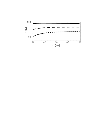
Figure 9: The fidelity of the quantum gate as a function of the inter-quantum dot separation $d$, for different values of the temperature $T$: 0 K (solid line), 5 K (long-dashed line), 15 K (dashed line).

The trion-trion shift is a crucial element of our quantum gate proposal. Its presence introduces the conditional dynamics. The timing of the adiabatic process should be designed in such a way that the trion-trion shift induces the required phase shift of the state $|e\rangle_{a}|e\rangle_{b}$.

The whole analysis of a single quantum dot operation can be easily generalized to the quantum gate case. As discussed above, we first transform into the dressed state basis and then select only “diagonal” terms from the interaction with the phonons. Then one can calculate the fidelity matrix $T$ (now $4\times 4$) and find the fidelity from Eq. (65). This program can be completed numerically.

Let us consider first the two simple limiting cases. In the simplest case of a small trion-trion shift $\Delta E_{ab}\ll\Omega$, the two quantum dots can be considered separately and the trion-trion shift can be accounted for as a perturbation. Then, following the steps of our single quantum dot calculation, we find that the infidelity is $f=1-\exp(-\Gamma)$, with

$$\Gamma=\int J(\omega)d\omega\cos^{2}(\omega d/u)[1+2N(\omega)]|a(\omega)|^{2},$$ (78)

where $a(\omega)$ is again given by Eq. (67). As expected, in this limit the result is practically the same as we had for a single qubit operation – see Eq. (66).

The dependence of the gate fidelity (78) on the quantum dots separation $d$ is very weak (the effective value of the $\cos$-function under the integral sign is anything between $1/2$ and $1$ for large and small values of $d$, respectively). This means that the obtained result is practically insensitive to the assumptions regarding the degree of coherence between the phonon modes around each of the dots. Indeed, Eq. (78) implies that both of the quantum dots interact with the same phonon bath. This corresponds to a case of having the dots interacting with the same set of bulk modes. Another possibility is that the inter-quantum dot separation is smaller than the phonon mean free path. In the case of separate phonon baths (which means the quantum dots electronic degrees of freedom interact with independent phonon modes, or the separation between the dots exceeds the mean free path of phonons), the quantum dots become completely separate and the infidelity is given by its single-qubit expression (66). Both expressions are indistinguishable within a factor $\sim 1$. The weak dependence of the fidelity on the interdot separation at not-too-high $T$ can be seen on the Fig. 9, obtained by our exact numerical calculation.

$\Omega$ (meV)	$f(T=0.1$ K)	$f(T=4$ K)	$f(T=20$ K)
0.3	$0$	$2.2\div 1.9\times 10^{-3}$	$5.9\div 4.5\times 10^{-3}$
0.06	$0$	$9.7\div 4.6\times 10^{-5}$	$4.8\div 2.3\times 10^{-4}$
0.02	$0$	$7.1\div 5.1\times 10^{-6}$	$5.3\div 2.5\times 10^{-5}$

Table 1: The infidelity $f(T)$ as a function of the temperature $T$ for different values of the Rabi frequency $\Omega$. The dot size is $20$ nm. The trion-trion shift $\Delta E_{ab}$ varies from $0.1$ meV to $3$ meV.

$\Omega$ (meV)	$f(T=0.1$ K)	$f(T=4$ K)	$f(T=20$ K)
0.3	$0$	$5.6\div 4.1\times 10^{-3}$	$0.034\div 0.020$
0.06	$0$	$5.0\div 4.6\times 10^{-5}$	$2.5\div 2.3\times 10^{-3}$
0.02	$0$	$1.5\div 1.4\times 10^{-5}$	$7.2\div 6.9\times 10^{-5}$

Table 2: The infidelity $f(T)$ as a function of the temperature $T$ for different values of the Rabi frequency $\Omega$. The dot size is $15$ nm. The trion-trion shift $\Delta E_{ab}$ varies from $0.1$ meV to $3$ meV.

$\Omega$ (meV)	$f(T=0.1$ K)	$f(T=4$ K)	$f(T=20$ K)
0.3	$0$	$1.4\div 0.92\times 10^{-2}$	$0.15\div 0.1$
0.06	$0$	$1.1\times 10^{-4}$	$1.2\times 10^{-3}$
0.02	N/A	N/A	N/A

Table 3: The infidelity $f(T)$ as a function of the temperature $T$ for different values of the Rabi frequency $\Omega$. The dot size is $10$ nm. The trion-trion shift $\Delta E_{ab}$ varies from $0.1$ meV to $3$ meV.

The calculation in the other limiting case $\Delta E_{ab}\gg\Omega$ is very similar. In this case the quantum gate has two avoided crossings instead of one and their contributions add independently. Since the width of the resonance is in both cases $\Omega$, the contributions of independent resonances add separately and are again of the same order of magnitude as Eq. (69) and (70). The dependence of the fidelity on the interdot separation is very weak again.

To quantify the discussion above we performed the exact numerical calculation of the fidelity matrix (62) using a certain shape of the detuning sweep $\Delta(t)$. The fidelity as a function of the interdot separation and of the temperature for a specific value of the trion-trion shift is plotted in Fig.(9). The figure nicely shows both temperature regimes (69) and (70), as well as the weak dependence of the result on the separation between the dots. We also performed a few calculations for quantum dots of different sizes (effectively varying the cutoff parameter $\omega_{l}$). The results of the calculations are summarized in the Tables (1)-(3). The interparticle separation is 5 nm, the pulse duration is 1 ps.

VII.8 Discussion

In this section we performed a systematic study of various decoherence mechanism associated with the interaction of the quantum dots with phonons. The results of our study can be summarized as follows.

The details of the interaction with phonons can be “compressed” into the spectral function $J(\omega)$. It is characterized by the strength of the coupling, the frequency dependence at small $\omega$ and the value of the high frequencies cutoff $\omega_{l}\sim u/l$, where $u$ is the velocity of sound and $l$ is the size of the quantum dot.

The infidelity $f$ turns out to be quite good for all the realistic situations we considered. This means that the perturbation theory is well applicable and, in the limit of small temperatures, the infidelity $f=1-\exp\{-\Gamma\}$ is given by

$$\Gamma\sim\frac{J(\omega_{c})}{\omega_{c}},$$ (79)

where $\omega_{c}=\min(\omega_{l},\omega_{m})$ and $\omega_{m}\sim\dot{\Delta}/\Omega$ is the inverse characteristic time of the gate operation. In the higher temperature limit ($T\gg\omega_{c}$) the infidelity scales linearly with the temperature

$$\Gamma\sim\frac{J(\omega_{c})}{\omega_{c}}\frac{T}{\omega_{c}}.$$ (80)

These expressions are the central results of the section. They can be applied to estimate the fidelities of both single qubit operations and of the quantum gates (in the latter case there is also a weak dependence on the separation between the quantum dots). The accuracy of the simple estimations along the lines of Eqs. (79) and (80) was checked by exact numerical calculations of the fidelity in a wide parameter range. The contributions of the piezoelectric coupling are numerically smaller by 2-3 orders of magnitude in all our calculations.

VIII State read-out by quantum jumps

A necessary requirement for a quantum information processing implementation scheme is the ability to perform an accurate measurement of a single qubit. Implementation of a highly efficient solid-state measurement scheme designed to measure the spin or charge of single electron is a highly difficult task Milburn01 .

Monitoring the fluorescence from a single quantum dot (QD) has been suggested as a mean to measure single scattering events within QDs Hohenester , as well as a means for final read out of the spin state for the purpose of quantum computation Imamoglu00 . Recently, it has been verified experimentally that the spin state of an electron residing in a QD can be read using circular pumped polarized light Cortez . In this section we describe how it is possible to devise an optical read out scheme based on the idea of the Pauli-blocking in QDs even in the presence of heavy/light hole mixing. We describe two situations: an ideal case with no heavy/light hole mixing and the realistic case which includes mixing. In the ideal case the time of measurement, i.e. the time in which one can still extract the information regarding the spin state of the confined electron, is limited only by the spin decoherence time whereas in the case of mixing the measurement time is also limited by the typical time for a spin flip induced by the excitation process.

The system we have in mind is described by Fig. 10. It is the single-QD counterpart of Eq. (IV.2), taking into account also the decay rates from the excited level, which we call $|x\rangle$ here for simplicity. We ignore the detunings $\delta$ and $\Delta$, which are not relevant here, as well as the decay rate $\kappa_{01}$ from state $|0\rangle$ to $|1\rangle$, since the typical time scale for it excitonspindeph is much larger than the typical time scale in which the spin directional information is lost due to the laser mediated spin flip which is now the bottleneck process limiting the measurement time.

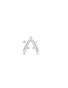
Figure 10: The lambda configuration one has to consider to include hole mixing.

VIII.1 Ideal case, i.e. no mixing

Let us first consider the case when $\varepsilon=0$. Shining a $\sigma^{+}$ pulse on the QD we obtain due to the Pauli blocking effect in QDs the usual two-level situation: no fluorescence from initial state $|0\rangle$, full fluorescence from state $|1\rangle$. The final state measurement i.e. measuring the spin state of the excess electron in the QD is obtained by the quantum jump technique (e.g. Ref. Imamoglu00 ): when the original state of the spin in a QD is $|1\rangle$ a fluorescence pattern is obtained, whereas the state $|0\rangle$ is completely decoupled from the laser field since exciton creation is blocked by the Pauli principle.

The typical time scale which limits the process is the spin coherence time in the QD which is of the order of microseconds, i.e. in a time of that order of a microsecond the spin of the electron in the QD will flip from the $|1\rangle$ fluorescing state to the $|0\rangle$ dark state and the fluorescence pattern will be terminated. The average number of photons emitted before the spin typically flips its state is given by the ratio of the spin coherence time to the typical rate for spontaneous emission, which is of the order of a few nano-seconds. Therefore, typically one should obtain on the order of $10^{3}$ photons before the original spin information is destroyed.

VIII.2 Case with mixing

A realistic QD will exhibit mixing of the heavy and light hole states. This invalidates the assumption of perfect Pauli blocking with $\sigma^{+}$ light and can be viewed as a rotation by an angle $-\varepsilon$ in the $\{|0\rangle,|1\rangle\}$ space. The mixing parameter $\varepsilon$ will typically be of the order of the lattice constant, $a$, to a typical length scale defining the QD in our case $a/L\approx 0.1$ where $L$ is the size of the dot in the growth direction.

Introducing mixing requires one to treat the full three-level lambda configuration shown in Fig. 10. As opposed to the usual atomic lambda configuration Zoller87 , here one can not distinguish between the $|0\rangle\langle x|$ and $|1\rangle\langle x|$ transitions. These two transitions are mediated through the same photon. The dissipative evolution of the density matrix $\tilde{\rho}(t)$ is given by Quantumnoise

$$\dot{\tilde{\rho}}_{00} = i\frac{\Omega}{2}\varepsilon\left(\tilde{\rho}_{x0}-\tilde{\rho}_{0x}\right)$$

$$\dot{\tilde{\rho}}_{11} = i\frac{\Omega}{2}\left(\tilde{\rho}_{x1}-\tilde{\rho}_{1x}\right)$$

$$\dot{\tilde{\rho}}_{xx} = i\frac{\Omega}{2}\left[\tilde{\rho}_{1x}-\tilde{\rho}_{x1}+\varepsilon\left(\tilde{\rho}_{0x}-\tilde{\rho}_{x0}\right)\right]-(1+\varepsilon^{2})\kappa\tilde{\rho}_{xx}$$

$$\dot{\tilde{\rho}}_{01} = i\frac{\Omega}{2}\left(\varepsilon\tilde{\rho}_{x1}-\tilde{\rho}_{0x}\right)$$ (81)

$$\dot{\tilde{\rho}}_{0x} = i\frac{\Omega}{2}\left[\varepsilon\left(\tilde{\rho}_{xx}-\tilde{\rho}_{00}\right)-\tilde{\rho}_{01}\right]-(1+\varepsilon^{2})\frac{\kappa}{2}\tilde{\rho}_{0x}$$

$$\dot{\tilde{\rho}}_{1x} = i\frac{\Omega}{2}\left(\tilde{\rho}_{xx}-\tilde{\rho}_{11}-\varepsilon\tilde{\rho}_{10}\right)-(1+\varepsilon^{2})\frac{\kappa}{2}\tilde{\rho}_{1x}$$

The probability that at time $t$ no photon has been emitted, starting from state $\alpha$ at time $t_{0}$, is

$$P^{(0)}_{\alpha}(t-t_{0})={\rm tr}\left[\tilde{\rho}(\alpha,t)\right],$$ (82)

where at the initial time $t_{0}$ we take $\tilde{\rho}(\alpha,t_{0})\equiv|\alpha\rangle\langle\alpha|$. Fig. 11 shows an example of their evaluation with $\Omega=3$ meV, $\kappa=1$ ns^-1 and $\varepsilon=0.1$.

Figure 11: Probability that at time $t$ the first photon has not yet been emitted, starting from state $|0\rangle$ (above) or $|1\rangle$ (below) at time $t=0$. Parameters are quoted in the text.

Note that, in contrast to the “common” lambda configuration Zoller87 , in Eq. (81) both of the recycling terms, $\kappa\tilde{\rho}_{xx}$ and $\varepsilon^{2}\kappa\tilde{\rho}_{xx}$, are missing, since it is the same photon that induces both these transitions, i.e. we can not distinguish between the two transitions via photon detection. This implies that, when the first photon is emitted, say at time $t_{1}$, the system collapses either into state $|0\rangle$ – with probability $p_{0}=\varepsilon^{2}/(1+\varepsilon^{2})$ – or into state $|1\rangle$ – with probability $p_{1}=1/(1+\varepsilon^{2})$ –, whence the evolution starts over again. Therefore the probability that, at the time $t>t_{i}$ ($i\geq 1$), the $(i+1)$-th photon has not been emitted, is

$$P^{(i)}_{\alpha}(t-t_{i})=\frac{\varepsilon^{2}P^{(0)}_{0}(t-t_{i})+P^{(0)}_{1}(t-t_{i})}{1+\varepsilon^{2}},$$ (83)

which is independent of the initial state $|\alpha\rangle$. A typical photoemission pattern will look like Fig. 12: a sequence of pulses, each one made out of a bunch of the order of $1/\varepsilon^{2}$ photons, separated by no-emission windows. This is the typical quantum-jump pattern one obtains in the presence of an emission probability having the form of a sum of different exponentials like Eq. (83).

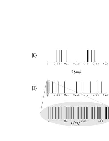
Figure 12: Simulation of photon counts for a system starting from state $|0\rangle$ (top) and from state $|1\rangle$ (middle). An expanded view of the first few photon counts is displayed in the bottom graph. Parameters are the same as in Fig. 11.

The only feature which allows for discriminating the two patterns is the first bunch of photons, which are emitted almost immediately in the case of state $|1\rangle$, and after a sensible delay in the case of state $|0\rangle$, due to the fact that, prior to the first photoemission, it was still $P^{(0)}_{0}(t)\not=P^{(0)}_{1}(t)$. Therefore, a detector with 100% efficiency would be still capable of discriminating between the two logical states even in the presence of hole mixing.

Another option would be available in II-VI semiconductor systems, showing energetic inversion between light and heavy hole states as described in Sect. VI. To be specific, let us refer to the left part of Fig. 8. In that case, the transition to be excited for probing the QD state is the one marked as (2). Hole mixing results in an unwanted coupling to the transition (1). This can be compensated for by simply adding a small component of $\sigma_{+}$ light, proportional to the mixing parameter $\varepsilon$. The error affecting this operation would scale linearly with the imprecision in $\varepsilon$, which is not straightforward to predict theoretically, yet it can be measured in a real situation to a good accuracy.

VIII.3 Case of perfect detection

We start by considering the error for the case $\eta=1$ where $\eta$ is the parameter describing the detection efficiency. On introducing hole mixing the detector would still be able to discriminate between the two logical states but mixing will be the cause for two types of measurement errors which can occur. Starting with the system in state $|1\rangle$ there is a possibility for no photon to be emitted from the QD during the whole measurement time. The probability for this type of error is given by: $P^{(0)}_{1}(t)$. In the other case starting with the system initially in $|0\rangle$ at least one photon might be emitted during the measurement time. The probability for this sort of error is given by: $1-P^{(0)}_{0}(t)$. The measurement time has to be chosen in such a way as to minimize the sum of these two errors. For the same parameters employed in Fig. 11, we obtain an estimate for the optimal measurement time of the order of a few tens of ns. What typically happens in practice is that, as shown in Fig. 12, by appropriate time windowing the first bunch of photons coming from state $|1\rangle$ can be safely discriminated from the (later) photons coming from state $|0\rangle$.

VIII.4 Finite detection efficiency

We now consider the case in which $\eta<1$. The lowest detector efficiency in which we can still hope to discriminate between the two logical states is given by $\eta=1/\langle N\rangle$, where remark  $\langle N\rangle=1/\varepsilon^{2}$ is the average number of photons to be emitted before a system starting off in state $|1\rangle$ flips to state $|0\rangle$. In our case this is not a tight constraint, since semiconductor photo-detectors have a very high quantum efficiency Bachor $\eta_{mat}\approx 0.98$. The typical wave length emitted by the recombination process in the QDs lies well within the spectral window which is due to the cutoff by band gap energy of such detectors. The main source for low detection efficiency is due to the probability for the emitted photon to reach the detector, i.e. the difficulty arising due to finite angle coverage of the detector. The situation however can be significantly improved by coupling the QD with a microcavity as described in Imamoglu00 .

It is important to note that we can use an avalanche photon counting mode so that each photon arriving creates one e-h pair which then amplifies in the device to produce a current spike. The need to wait a few nanoseconds before detecting the next photon is not a limitation in our case since the measurement process we are considering is essentially a one shot measurement process, as long as the dark count is low enough.

Working with a detector with a finite efficiency means that we have to choose the measurement time so as to ensure the fluorescent state emits a few photons thus increasing the probability one of them will be detected. This increases the probability for an error due to a photon being emitted by the initial state $|0\rangle$ since $P^{(0)}_{0}(t)$ decays exponentially with time. Moreover a further possibility for error is introduced into our measurement scheme. Starting initially in state $|1\rangle$ the QD can emit a photon/photons which will go undetected and the spin can flip into state $|0\rangle$, i.e., the information regarding the spin state is lost without being detected. The probability $P_{e}$ for such an error is given by

$$P_{e} = \varepsilon^{2}\sum_{n=0}^{N}\left(\frac{1-\eta}{1+\varepsilon^{2}}\right)^{n+1}$$ (84)

$$= \frac{\varepsilon^{2}(1-\eta)}{\varepsilon^{2}+\eta}\left[1-{\left({1-\eta\over 1+\varepsilon^{2}}\right)}^{N+1}\right],$$

which is simply the sum over $n$ incidents in which the emitted photons were not detected and no spin-flip occurred and on the $n+1$ incident such a spin flip occurred (without the photon being detected). This type of error turns out not to be particularly sensitive to the time of measurement. Given that the number of photon emitted in the first bunch in Fig. 12 is of the order of $\varepsilon^{-2}\approx 10^{2}$ in our case as discussed above, and taking an efficiency $\eta=0.9$ we obtain an error due to finite detection efficiency of the order of 0.1%.

IX Conclusions

To claim that a certain implementation scheme for quantum information processing is viable, one has to carefully understand the fundamental sources of decoherence acting in that specific physical system, and to show that they can actually be controlled. To this aim, in this paper we analyzed in detail the different decoherence mechanisms affecting a recently proposed all-optical scheme for quantum computation based on electron spin in quantum dots. In particular, we took into account the effect of hole mixing and of coupling to phonons at a finite temperature, estimating their impact on each of the building blocks of a quantum computer: single- and two-qubit gates, and state read-out. We developed a strategy to circumvent such unwanted effects via an adiabatic laser excitation scheme, simulated its performance under realistic conditions and evaluated the corresponding fidelity. Our scheme turns out to be able to suppress the effect of both of these decoherence sources on the proposed gate, and therefore constitutes a viable proposal for all-optical quantum information processing in semiconductor quantum dots.

Appendix A Coupling constants: Microscopic calculation

The phonons are coupled to the charge distribution in a QD by means of either deformation or piezoelectric coupling potentials. The corresponding coupling constants are either

$$\lambda_{q}^{D}=\frac{qD(q)}{\sqrt{2\rho\omega(\mathbf{q})V}}$$ (85)

in the case of deformation coupling, or

$$\lambda_{\mathbf{q}}^{p}=\frac{\rho(\mathbf{q})}{\sqrt{2\rho\omega(\mathbf{q})V}}M(\mathbf{q}),$$ (86)

in the case of piezoelectric coupling. In both cases $\rho$ is the mass density of the sample, and

$$M(\mathbf{q})=\frac{24\pi ee_{14}}{\epsilon q^{3}}q_{x}q_{y}q_{z}\equiv M\frac{q_{x}q_{y}q_{z}}{q^{3}},$$ (87)

is the coupling potential. Here $\epsilon$ is the dielectric constant of the sample and $e_{14}$ is the material constant. The form-factors

$$\rho(\mathbf{q})=\int d\mathbf{r}\big{[}|\psi_{v}(\mathbf{r})|^{2}-|\psi_{c}(\mathbf{r})|^{2}\big{]}\exp(-i\mathbf{q}\mathbf{r}),$$ (88)

and takagahara

$$D(\mathbf{q})=\int d\mathbf{r}\big{[}D_{v}|\psi_{v}(\mathbf{r})|^{2}-D_{c}|\psi_{c}(\mathbf{r})|^{2}\big{]}\exp(-i\mathbf{q}\mathbf{r})$$ (89)

are related to the exciton charge density. The wavefunctions $\psi_{v}$and $\psi_{c}$ describe the hole and the electron states making up the exciton. $D_{c},D_{v}$ are the deformation coupling potentials.

The calculation of the coupling constants relies on a microscopic model. We consider a QD in a static external electric field $F_{0}$ directed along the $x$-axis. Within the simplest model with harmonic confinement potential the Hamiltonian for the single-particle electron ($i=e$) and the holes ($i=h$) states is given by

$$H=\frac{p^{2}}{2m_{i}}+\frac{m_{i}\omega_{i}^{2}(r+r_{0i})^{2}}{2}-\frac{m_{i}\omega_{i}^{2}r_{0i}^{2}}{2},$$ (90)

where $r_{0i}=e_{i}F_{0}/m_{i}\omega_{i}^{2}$ is a measure of the electric field strength in “oscillator units of length”, $\omega_{i}$ is the frequency of the confining potential, $m_{i}$ and $e_{i}$ are the mass and the charge of the particles (the electrons or holes).

To clarify the effects of external electric field and compare the relative strength of the different types of the coupling, let us consider first the somewhat unrealistic but otherwise simple model of a spherically symmetric QD. In this case the wavefunction is given by

$$\psi_{i}=\left(\frac{1}{\pi l_{i}^{2}}\right)^{3/2}\exp\left\{-\frac{(\mathbf{r}-\mathbf{r}_{0i})^{2}}{2l_{i}^{2}}\right\},$$ (91)

where $l_{i}=(m_{i}\omega_{i})^{-1/2}$ is the ground state localization length. Then, in the case of deformation coupling, a simple calculation gives the following expression for $J-$function (for simplicity we put $l_{e}=l_{h}$):

$$J(\omega) = \frac{\omega^{3}}{4\pi^{2}\rho u^{5}}\exp\Bigl{\{}-\frac{\omega^{2}l^{2}}{2u^{2}}\Bigr{\}}$$ (92)

$$\mbox{}\times\Bigl{[}D_{e}^{2}+D_{h}^{2}-2D_{e}D_{h}\frac{\sin(2\omega r_{0}/u)}{2\omega r_{0}/u}\Bigr{]}.$$

The obtained result shows the two important features. First of all, since $D_{e}\neq D_{h}$ the $J-$function is superohmic in the external field of any strength. Essentially this means that a static electric field does not qualitatively change the interaction with the phonons. Secondly, the function $J(\omega)$ has a large frequency cutoff at $\omega_{l}=u/l$, which is nothing else but the inverse flight time of a phonon through the QD.

The piezoelectric coupling behaves somewhat different. Recalculating the $J-$function using the coupling constant (86) we find

$$J^{p}(\omega) = \frac{M^{2}\omega}{560\pi^{2}\rho u^{3}}\Bigl{[}\exp\Bigl{(}-\frac{\omega^{2}l_{c}^{2}}{2u^{2}}\Bigr{)}+\exp\Bigl{(}-\frac{\omega^{2}l_{v}^{2}}{2u^{2}}\Bigr{)}$$ (93)

$$- 2\exp\Bigl{(}-\frac{\omega^{2}l_{c}^{2}}{4u^{2}}\Bigr{)}\exp\Bigl{(}-\frac{\omega^{2}l_{v}^{2}}{4u^{2}}\Bigr{)}f\Bigl{(}2\frac{\omega}{u}r_{0}\Bigr{)}\Bigr{]}$$

where $f(0)=1$ and $f(x)\rightarrow 0$ at $x\rightarrow\infty$. Since the piezoelectric potential $M$ is the same for the electrons and for the holes, in the limit of small electric field strength we have:

$$J_{F_{0}=0}^{p}(\omega\rightarrow 0)=\frac{M^{2}\omega^{5}(l_{c}^{2}-l_{v}^{2})^{2}}{6720\pi^{2}\rho u^{7}}.$$ (94)

The coupling is still superohmic, but it contains a larger power of $\omega$ than the deformation coupling. Moreover, the value of the coupling potential $M$ is also numerically small for common materials and thus the interaction of a QD with the phonons is dominated by the deformation coupling.

The large electric field limit of Eq. (93) is somewhat interesting. One can see that we have

$$J_{F_{0}=\infty}^{p}(\omega\rightarrow 0)=\frac{M^{2}\omega}{280\pi^{2}\rho u^{3}},$$ (95)

which is, at first glance, an indication of ohmic type of coupling. Nevertheless, one should keep in mind that the $J^{p}-$function decreases quickly when $\omega\gtrsim\omega_{l}$ and hence the argument of the $f$-function never exceeds $\sim r_{0}/l$. This means that the function $f\sim 1$ practically everywhere in the course of the integration in Eq. (48) and hence the coupling remains superohmic in the whole relevant parameters range.

The analysis above paves the way to a more realistic calculation. Consider the Hamiltonian (90) acting in 2D ($x$- and $y$- directions), whereas the motion in the $z$-direction is confined within a box of length $L_{z}$. The wavefunction (of the ground state) is

$$\psi_{i}=\sqrt{\frac{2}{L_{z}}}\sin\frac{\pi z}{L_{z}}\sqrt{\frac{m_{i}\omega_{i}}{\pi}}\exp\Bigl{\{}-\frac{(r+r_{0i})^{2}}{2l_{i}^{2}}\Bigr{\}},$$ (96)

where $l_{i}=\sqrt{m_{i}\omega_{i}}$. The Fourier component is given by

$$\int d^{3}r\psi^{2}\exp\{-i\mathbf{q}\mathbf{r}\}=F_{z}(q_{z})F(\mathbf{q}),$$ (97)

where $\mathbf{q}=(q_{x},q_{y})$ is the vector in the $xy-$plane, and

$$F(\mathbf{q})=\exp\Bigl{\{}-\frac{q^{2}l^{2}}{4}+i\mathbf{q}\mathbf{r}_{0}\Bigr{\}},$$ (98)

and

$$F_{z}(q_{z})=\frac{4\pi^{2}i[\exp(iq_{z}L)-1]}{(q_{z}L)^{3}-4\pi^{2}q_{z}L}.$$ (99)

We note that, in spite of its ugly appearance, the form-factor $F_{z}$ is nowhere singular on the real axis and quickly decays when $q_{z}L\gg 1$. The normalization ensures that $F_{z}(0)=1$.

For simplicity consider the limit of very strong confinement: $L_{z}\ll l_{c,v}$. Then, neglecting the piezoelectric coupling and using the zero-argument value for the function $F_{z}$, we obtain

$$J(\omega)=\frac{\omega^{3}}{4\pi^{2}\rho u^{5}}\exp\Bigl{\{}-\frac{\omega^{2}l^{2}}{2u^{2}}\Bigr{\}}\Bigl{[}D_{c}^{2}+D_{v}^{2}-2D_{c}D_{v}f_{1}\Bigl{(}2\frac{\omega}{u}r_{0}\Bigr{)}\Bigr{]},$$ (100)

where we have

$$f_{1}(x)=\frac{1}{4\pi}\int d\theta\sin\theta\;d\phi\;\cos(x\sin\theta\cos\phi).$$ (101)

At small value of its argument this function gives $1$ and vanishes when $x\rightarrow\infty$. The presented $J-$function is always superohmic and is not qualitatively different from that considered above for an idealistic spherically symmetric QD. It shares all the important features of the simpler model above. In particular, the large-frequency cutoff is defined by the same inverse phonon flight-time through the QD: $\omega_{l}\sim u/l$.

In short, we presented a number of examples of the spectral function calculations. Both in the case of piezoelectric and of deformation coupling, the $J$-function is superohmic, with the exponents $s=3$ and $s=5$, respectively. The quantity $\omega_{l}\sim u/l$ plays the role of the high frequency cutoff.

Appendix B Adiabatic effective Hamiltonian: Applicability of perturbation expansions

The phonon interaction terms in the Hamiltonian (47) may well be large and hence the perturbation theory expansion in powers of $\lambda_{\mathbf{q}}$ may not always be well justified. A remarkable opportunity to extract non-perturbative results originates from our adiabatic assumption.

Indeed our quantum gate proposal relies on adiabatic manipulations of the external parameters of the Hamiltonian (47). Assume that both $\Omega(t)$ and $\Delta(t)$ change on a time scale $\tau$. Extreme adiabatic condition implies

$$\omega_{l}\tau\gg 1,$$ (102)

i.e. the considered QD dynamics can be considered slow for almost all of the phonon modes. According to Leggett , this condition can be formally used to adiabatically eliminate all the phonon modes with frequencies exceeding a certain cutoff $\omega_{*}$: $\tau^{-1}\ll\omega_{*}\ll\omega_{l}$ and obtain the effective adiabatic Hamiltonian for the slow phonon modes with frequencies $\omega\lesssim\omega_{*}$. At zero temperature $T=0$ the effective Hamlitonian takes the form:

$$H_{\rm ph} = \Bigl{[}-\tilde{\Delta}+\sum_{\mathbf{q},\omega(\mathbf{q})<\omega_{*}}\lambda_{\mathbf{q}}(b_{\mathbf{q}}+b_{\mathbf{q}}^{\dagger})\Bigr{]}|e\rangle\langle e|$$

$$+\frac{\tilde{\Omega}}{2}(|e\rangle\langle g|+|g\rangle\langle e|)+\sum_{\mathbf{q},\omega(\mathbf{q})<\omega_{*}}\omega(\mathbf{q})b_{\mathbf{q}}^{\dagger}b_{\mathbf{q}}.$$

The Hamiltonian (B) has the same form as the original Hamiltonian (47). The effect of the high frequency mode is limited to the renormalization of the frequency detuning

$$\tilde{\Delta}=\Delta-\frac{1}{2}\int d\omega\frac{J(\omega)}{\omega},$$ (104)

and Rabi frequency (tunneling term in the spin boson model)

$$\tilde{\Omega}=\Omega\exp\left(-\int_{\omega_{*}}^{\infty}\frac{d\omega}{2}\frac{J(\omega)}{\omega^{2}}\right),$$ (105)

In the superohmic case the integral in the exponent of Eq. (105) converges at $\omega\lesssim\omega_{*}$ and hence does not depend on $\omega_{*}$. Thus, in the adiabatic approximation we can conveniently set $\omega_{*}=0$. This means that at zero temperature even a strong phonon coupling leads only to the renormalization of the Hamiltonian parameters (the Rabi frequency). The measure of the Rabi frequency renormalization yields the perturbation theory expansion parameter:

$$\frac{\Omega-\tilde{\Omega}}{\Omega}\sim\int\frac{d\omega}{2}\frac{J(\omega)}{\omega^{2}}\sim\frac{J(\omega_{l})}{\omega_{l}}\ll 1.$$ (106)

The effective Hamiltonian (B) does not rely on this condition, whereas a perturbation theory for arbitrary fast processes would do.

The situation is somewhat different at finite temperatures. The QD can still change its state “coherently”, i.e. in the course of Rabi oscillations which are characterized by the new temperature-dependent renormalized value, called Huang-Rhys factor in Leggett :

$$\tilde{\Omega}=\Omega\exp\Bigl{\{}-\int_{0}^{\infty}\frac{d\omega}{2}\frac{J(\omega)}{\omega^{2}}[1+2N(\omega)]\Bigr{\}},$$ (107)

where $N(x)=[\exp(x/T)-1]^{-1}$ is the Bose occupation number. This is nothing else but the generalization of Eq. (105) now taking into account finite occupation of the phonon modes. In addition to that, the QD can change its state by either absorbing or emitting a phonon. This process is called incoherent tunnelling and has no effective Hamiltonian form (generally speaking there is no obvious separation between the fast and slow variables).

In the quantum gate proposal we suggest to operate our qubit starting from the ground state and adiabatically changing parameters. This means that the QD cannot emit a phonon of a high energy $\omega\gtrsim\tau^{-1}$ (since it is in the ground state). The absorption of a phonon from the thermal bath requires finite occupancy of a state with energy $\omega\sim\tilde{\Omega}$, which can be made exponentially small, provided $T\ll\tilde{\Omega}$.

The results of this section also make sense if compared with perturbation theory. Consider the case of the phonon coupling. There is no corrections to the eigenenergies (37) to first order in powers of $\lambda_{q}$. The second order perturbation theory gives

$$\delta E_{\pm}=\sum_{q}\frac{\lambda_{q}^{2}}{4}\left\{\frac{[1\pm\cos(\theta)]^{2}}{\omega_{q}}+\frac{\sin^{2}(\theta)}{\sqrt{\Delta^{2}+\Omega^{2}}+\omega_{q}}\right\}.$$ (108)

In the adiabatic limit (102) we can expand in powers of $\Delta/\omega_{l}$ and $\Omega/\omega_{l}$ to obtain the expression:

$$\delta E_{\pm} = \frac{1}{2}(1\pm\cos\theta)\int d\omega\frac{J(\omega)}{\omega}$$ (109)

$$\mbox{}-\frac{\sin^{2}\theta}{4}\sqrt{\Delta^{2}+\Omega^{2}}\int d\omega\frac{J(\omega)}{\omega^{2}}.$$

The same expression could be obtained by substituting the renormalized values (104-105) into the adiabatic energies (37) and expanding the obtained expession in powers of the small parameter (106). This once again shows that the results of the adiabatic renormalization coincide with perturbation theory whenever both approaches are equally valid.

We conclude that the effective Hamiltonian (B) with renormalized value of the Rabi transition amplitude (107) can be used as a good non-perturbative tool to study the QD dynamics in the presence of phonons. Its validity is ensured by the fact that the $J$-function for the deformation coupling is superohmic and relies on the timescale separation condtion (102). In the case when $\omega_{l}\tau\gtrsim 1$, the adiabatic approximation fails and one has to resort to perturbation theory, whose expansion parameter is given by (106).

References

- (1) Fort. Phys. 48, Nos. 9-11 (2000).
- (2) E. Knill , E. Laflamme, Phys. Rev. A 55, 900 (1997): D. Gottesman, Phys. Rev. A 52, 1862 (1996); A. R. Calderbank, E. M. Rains, P. W. Shor and N. J. A. Sloane, Phys. Rev. Lett. 78, 405 (1997).
- (3) L. M. Duan and G. C. Guo, Phys. Rev. Lett. 79, 1953 (1997); P. Zanardi and M. Rasetti, ibid. 79, 3306 (1997); D. A. Lidar, I. L. Chuang and K. B. Whaley, ibid. 81, 2594 (1998); E. Knill, R. Laflamme and L. Viola, ibid 84, 2525 (2000).
- (4) T. Calarco, J. I. Cirac, and P. Zoller, Phys. Rev. A 63, 062304 (2001).
- (5) E. Pazy, T. Calarco, I. D’Amico, P. Zanardi, F. Rossi and P. Zoller, submitted; E. Pazy, E. Biolatti, T. Calarco, I. D’Amico, P. Zanardi, F. Rossi and P. Zoller, J. Supercond. (to be published).
- (6) A. V. Khaetskii and Y. V. Nazarov Phys. Rev. B 61, 12639 (2000).
- (7) B. Krummheuer, V. M. Axt, and T. Kuhn, Phys. Rev. B 65, 195313 (2002); E. Pazy, Semicond. Sci. Tech. 17 1172 (2002); L. Jacak, A. Janutka, P. Machnikowski, A . Radosz, Preprint cond-mat/0212057.
- (8) E. Biolatti, RC. Iotti, P. Zanardi and F. Rossi, Phys. Rev. Lett. 85, 5647 (2000); S. De Rinaldis, I. D’Amico, E. Biolatti, R. Rinaldi, R. Cingolani, F. Rossi, Phys. Rev. B 65, 081309(R) (2002).
- (9) D. Loss and D. P. DiVincenzo, Phys. Rev. A 57, 120 (1998).
- (10) D. Jaksch, J. I. Cirac, P. Zoller, S. L. Rolston, R. Cote and M. D. Lukin, Phys. Rev. Lett. 85, 2208 (2000).
- (11) S. Bandyopadhyay, Phys. Rev. B 61, 13813 (2000); T. Tanamoto, Phys. Rev. A 61, 022305 (2000); J. H. Reina, L. Quiroga and N. F. Jhonson, Phys. Rev. A 62, 012305 (2000); F. Troiani, U. Hohenester, E. Molinari, Phys. Rev. B 62, R2263 (2000); it ibid, Phys. Stat. Sol. B 224, 849 (2001); K. R. Brown, D. A. Lidar, K. B. Whaley Phys. Rev. A 65, 012307 (2002).
- (12) G. Bukard, D. Loss, D. P. Divincenzo, Phys. Rev. B 59, 2070 (1999); J. Schliemann, D. Loss and A.H. MacDonald, Phys. Rev. B 63, 085311 (2001); G. Burkard and D. Loss, Phys. Rev. Lett. 88, 047903 (2002); V. N. Golovach and D. Loss, Semicond. Sci. Technol. 17, 355 (2002).
- (13) X. D. Hu and S. Das Sarma, Phys. Rev. A 61, 062301 (2000); ibid, 64, 042312 (2001); M. Bayer, P. Hawrylak, K. Hinzer, S. Fafard, M. Korkusinski, Z. R. Wasilewski, O. Stern and A. Forchel, Science 291, 451 (2001).
- (14) A. Imamoğlu, Fortschr. Phys. 48, 987 (2000).
- (15) A. Imamoğlu, D. D. Awschalom, G. Bukard, D. P. DiVincenzo, D. Loss, M. Sherwin and A .Small, Phys. Rev. Lett. 83, 4204 (1999); A. Kiraz, P. Michler, C. Becher, B. Gayral, A. Imamoğlu, Lidong Zhang, E. Hu, W. V. Schoenfeld and P. M. Petroff, Appl. Phys. Lett. 78, 3932 (2001).
- (16) C. Piermarocchi, Pochung Chen, L. J. Sham and D. G. Steel, Phys. Rev. Lett. 89, 167402 (2002);
- (17) T. H. Stievater, X. Q. Li, D. G. Steel, D. Gammon, D. S. Katzer, D. Park, C. Piermarocchi and L. J. Sham, Phys. Rev. Lett. 87, 133603 (2001); H. Kamada, H. Gotoh, J. Temmyo, T. Takagahara, H. Ando, ibid 87, 246401 (2001); A. Zrenner, E. Beham, S. Stufler, F. Findeis, M. Bichler and G. Abstreiter, Nature 418, 612 (2002).
- (18) J. R. Guest, T. H. Stievater, Gang Chen, E. A. Tabak, B. G. Orr, D. G. Steel, D. Gammon, D. S. Katzer, Science 293, 2224 (2001).
- (19) P. Y. Yu and M. Cardona, Fundamentals of Semiconductores (Springer ,Berlin, 2001).
- (20) See, e.g., L. Jacak and P. Hawrylak and Wojs, Quantum Dots (Springer, Berlin, 1998).
- (21) F. Rossi, Semicond. Sci. Technol. 13, 147 (1998).
- (22) E. Biolatti, I. D’Amico, P. Zanardi and F. Rossi, Phys. Rev. B 65, 075306 (2002).
- (23) U. Banin, Y. Cao, D. Katz and O. Millo, Nature 400, 542 (1999).
- (24) G. Bastard, Wave mechanics applied to semiconductor heterostructures (Les Ulis Cedex,1998).
- (25) H. Haug and S. W. Koch, Quantum theory of the optical and electronic proporties of semiconductors (World Scientific, Singapore, 1993).
- (26) F. Findeis, M .Baier, A. Zrenner, M. Bichler, G. Abstreiter, U. Hohenester and E. Molinari, Rev. B 63, 121309 (2001); D. V. Regelman, E. Dekel, D. Gershoni, E. Ehrenfreund, A. J. Williamson, J.Shumway, A. Zunger, W.V. Schoenfeld and P. M. Petroff Phys. Rev. B 64, 165301 (2001); A. Kiraz, S. Falth, C. Becher, B. Gayral, W. V. Schoenfeld, P. M. Petroff, Lidong Zhang, E. Hu, and A. Imamoğlu, Phys. Rev. B. 65, 161303 (2002).
- (27) R. J. Warbuton, C. S. Dürr, K. Karrai, J.P. Kotthaus, G. Medeiros-Ribeiro and P. M. Petroff, Phys. Rev. Lett. 79, 5282 (1997); V. K. Kalevich, M. Paillard, K. V. Kavokin, X. Marie, A. R. Kovsh, T. Amand, A. E. Zhukov, Yu. G. Musikhin, V. M. Ustinov, E. Vanelle and B. P. Zakharchenya, Phys. Rev. B. 64, 045309 (2001). Gang Chen, N. H. Bonadeo, D. G. Steel, D. Gammon, D. S. Katzer, D. Park and L. J. Sham, Science 289, 1906 (2000).
- (28) J. M. Luttinger Phys. Rev. 102, 1030 (1956).
- (29) D. P. DiVincenzo, D.Bacon, J. Kempe, G. Burkard and K. B. Whaley, Nature 408, 339 (2000).
- (30) E. Perez, V. Bellani, S. Zimmermann, L. Munoz, L. Vina, E. S. Koteles and K. M. Lau, Solid State Electronics 40, 737 (1996).
- (31) J. S. Weiner,D. S. Chemla,D. A. B. Miller, H. A Haus,A. C. Gossard, W. Wiegmann and C. A. Burrus, Appl. Phys. Lett. 47, 664 (1985).
- (32) D. Gammon, E. S. Snow, B. V. Shanabrook, D. S. Katzer and D. Park, Science 273, 87 (1996); M. Bayer and A. Forchel, Phys. Rev. B 65, 041308 (2002).
- (33) I. Wilson Rae and A. Imamoğlu, Phys. Rev. B 65, 235311 (2002).
- (34) A. J. Leggett, S. Chakravarty, A. T. Dorsey, M. P. Fisher, A. Garg, and W. Zwerger, Rev Mod. Phys. 59, 1 (1987); A. Wurger, Phys. Rev B 57, 347 (1997).
- (35) L. D. Landau and E. M. Lifshitz, Quantum Mechanics, (Pergamon Press, Oxford, 1997), Sec. 53,90.
- (36) H. -S. Goan and G. J. Milburn, Phys. Rev B 64, 235307 (2001).
- (37) U. Hohenester, Solid State Commun. 118, 151 (2001).
- (38) S. Cortez, O.Krebs, S. Laurent, M. Senes, X. Marie, P. Voisin, R. Ferreira, G. Bastard, J. M. Gerard and T. Amand, Phys. Rev. Lett. 89, 207401-1 (2002).
- (39) H. Kamada, H. Gotoh, H. Ando, J. Temmyo and T. Tamamura, Phys. Rev. B. 60, 5791 (1999); H. Gotoh, H. Ando, H. Kamada, A. Chavez-Pirson and J. Temmyo Appl. Phys. Lett. 72, 1341 (1998); M. Paillard, X. Marie, P. Renucci, T. Amand, A. Jbeli and J. M. Gérard, Phys. Rev. Lett. 86, 1634 (2001).
- (40) P. Zoller, M. Marte, D.F. Walls, Phys. Rev. A 35, 198 (1987).
- (41) See, e.g., C. W. Gardiner and P. Zoller Quantum Noise, 2nd ed. (Springer,2000).
- (42) The value of is given by , where and .
- (43) See, e.g., H.-A. Bachor A Guide to Experiments in Quantum Optics (Wiley-VCH, Weinheim, 1998).
- (44) T. Takagahara, Phys. Rev. B 60, 2638 (1999).