A new method for the solution of the Schrödinger equation

Abstract

We present a new method for the solution of the Schrödinger equation applicable to problems of non-perturbative nature. The method works by identifying three different scales in the problem, which then are treated independently: An asymptotic scale, which depends uniquely on the form of the potential at large distances; an intermediate scale, still characterized by an exponential decay of the wave function and, finally, a short distance scale, in which the wave function is sizable. The key feature of our method is the introduction of an arbitrary parameter in the last two scales, which is then used to optimize a perturbative expansion in a suitable parameter. We apply the method to the quantum anharmonic oscillator and find excellent results.

In this Letter we present a new method to find approximate solutions to eigenvalue problems in Quantum Mechanics. In particular, this method is applicable to problems where ordinary perturbation theory generates divergent asymptotic series. Actually, improving the convergence of the standard Rayleigh-Schrödinger perturbative expansion has been the subject of many studies in the past (see, e. g., Refs. Hatsuda:1996vp ; BB96 ; Gui95 ; Jan95 and references therein) and many variants of “optimized expansions” have been proposed.

Among them we would like to single out the Linear Delta Expansion (LDE) lde , which is at the base of our developments. The LDE has been extensively applied in many different settings with varying degrees of success. For example, in Ref. blencowe it has been used to analyze disordered systems. In Ref. Jones:2000au it has been applied to study the slow roll potential in inflationary models. Pinto and collaborators have applied it to the Bose-Einstein condensation problem Kneur:2002dn , the $O(N)(\phi^{2})^{2}_{3d}$ model Kneur:2002kq , the Walecka model Krein:1995rp and to the $\phi^{4}$ theory at high temperature Pinto:1999py . More recently the LDE has been applied with success to the study of classical nonlinear systems AA1:03 ; AA2:03 . Detailed references on the method can be found in these works.

Here, we illustrate the method we propose by applying it to the quantum anharmonic oscillator, which is the usual benchmark to test any non-perturbative method.

The cornerstone of the method is the identification of three different scales in the problem, which give rise to different behaviors of the wave function. Keeping in mind the standard separation of the Hamiltonian in a unperturbed piece (the harmonic oscillator) and a perturbative one (the anharmonic term), one can recognize that at very large distances the wave function assumes its asymptotic behavior: This is completely determined by the anharmonic potential and it is the same for all (ground and excited) states; at intermediate distances the wave function still decays exponentially, but now governed by the harmonic term; finally, there is a short distance scale, in which the wave function is sizable.

The key feature of our method is the introduction of an arbitrary parameter in the last two scales, which is then used, in the LDE spirit, to optimize a perturbative expansion in a suitable parameter.

Consider the Schrödinger equation

$$\left[-\frac{\hbar^{2}}{2m}\frac{\partial^{2}}{\partial x^{2}}+\frac{m\omega^{2}}{2}x^{2}+\frac{\mu}{4}x^{4}\right]\psi_{n}(x)=E_{n}\psi_{n}(x),$$ (1)

where $\mu$ is the anharmonic coupling. The asymptotic behavior of $\psi_{n}(x)$ in the region of large $x$ is determined by substituting the ansatz $\psi_{n}(x)\propto e^{-\gamma|x|^{p}}$ into Eq. (1). One obtains $p=3$ and $\gamma=\sqrt{\mu m/2}/3\hbar$.

In order to make the three scales explicit in the wave function, we write

$$\psi_{n}(x)=e^{-\gamma|x|^{3}-\beta x^{2}}\xi_{n}(x),$$ (2)

where the exponential takes care of the correct behavior in the limit $|x|\rightarrow\infty$. Notice that the quadratic term in the exponential does not affect the behavior at large distances, but dominates at scales where $|x|<\beta/\gamma$. Here $\beta=m\sqrt{\omega^{2}+\Omega^{2}}/2\hbar$ is the coefficient of a harmonic oscillator of frequency $\tilde{\Omega}\equiv\sqrt{\omega^{2}+\Omega^{2}}$, where $\Omega$ is an arbitrary parameter introduced by hand; $\xi_{n}$ is a well-behaved function, which fulfills the equation :

$$\xi_{n}^{\prime\prime}(x) - \left[\frac{\sqrt{2m\mu}}{\hbar}x^{2}+\frac{2m\widetilde{\Omega}x}{\hbar}\right]\xi^{\prime}_{n}(x)$$ (3)

$$+ \left[\frac{\sqrt{2\mu m^{3}\widetilde{\Omega}^{2}}}{\hbar^{2}}x^{3}+\frac{m^{2}\Omega^{2}}{\hbar^{2}}x^{2}-\frac{\sqrt{2m\mu}}{\hbar}x\right.$$

$$+ \left.\frac{2mE_{n}}{\hbar^{2}}-\frac{m\widetilde{\Omega}}{\hbar}\right]\xi_{n}(x)=0.$$

Equation (2) has been introduced in order to single out three different regimes in the wave function: The purely asymptotic regime ($|x|\rightarrow\infty$), where the cubic term in the exponential dominates; the intermediate regime, where $|x|$ is not yet asymptotic but large enough to expect the wave function to be exponentially damped; the regime of small $|x|$ where the physics is all contained in the $\xi$’s. The last two regimes will display a dependence upon the arbitrary frequency $\Omega$, although in a quite different fashion (in fact, the intermediate regime displays a truly non-perturbative dependence upon $\Omega$). In the limits $(\mu,\Omega)\rightarrow 0$ one obtains the equation for the harmonic oscillator of frequency $\omega$, which admits polynomial solutions (the Hermite polynomials).

It is worth stressing that the energy $E_{n}$ in Eq. (3) is still the true energy, since no approximation has been used to derive this equation.

We observe in Eq. (3) that both the wave function $\xi_{n}(x)$ and the energy $E_{n}$ depend in some nontrivial way upon the anharmonic coefficient $\mu$. On the other hand, the dependence of $\psi_{n}(x)$ and $E_{n}$ upon the arbitrary frequency $\Omega$ is only fictitious, since this parameter does not appear in the original equation (1). Nonetheless, we will show that $\Omega$ can be used to generate an efficient expansion for the solution of Eq. (1).

Indeed we rewrite Eq. (3) as

$$\xi_{n}^{\prime\prime}(x) - \left[\frac{2m\widetilde{\Omega}x}{\hbar}\right]\xi^{\prime}_{n}(x)+\left[\frac{2mE_{n}}{\hbar^{2}}-\frac{m\widetilde{\Omega}}{\hbar}\right]\xi_{n}(x)$$ (4)

$$= \delta\left\{\frac{\sqrt{2m\mu}}{\hbar}x^{2}\xi^{\prime}_{n}(x)-\left[\frac{\sqrt{2\mu m^{3}\widetilde{\Omega}^{2}}}{\hbar^{2}}x^{3}\right.\right.$$

$$+ \left.\left.\frac{m^{2}\Omega^{2}}{\hbar^{2}}x^{2}-\frac{\sqrt{2m\mu}}{\hbar}x\right]\xi_{n}(x)\right\},$$

where the left hand side of Eq. (4) corresponds to the equation for a harmonic oscillator of frequency $\widetilde{\Omega}$. Following the spirit of the LDE, we have introduced a parameter $\delta$, which is going to be used as a power-counting device: When $\delta=1$, Eq. (4) reduces exactly to Eq. (3).

Although $\delta$ is not a small parameter we will treat the right hand side of Eq. (4) as a perturbation, writing down the following expansions:

$$\xi_{n}(x)=\sum_{j=0}^{\infty}\delta^{j}\xi_{nj}(x),\ \ E_{n}=\sum_{j=0}^{\infty}\delta^{j}E_{nj}.$$ (5)

Combining Eqs. (4) and (5), one can generate a hierarchy of equations, corresponding to the different orders in $\delta$.

Since we are doing perturbation theory, all the results, to any finite order in the expansion, will depend upon the arbitrary frequency $\Omega$. Such dependence will therefore be minimized by applying the Principle of Minimal Sensitivity (PMS) Ste81 , i.e. by requiring that a given observable $O$ (the energy, for example) be locally independent of $\Omega$:

$$\frac{\partial O}{\partial\Omega}=0.$$ (6)

We will illustrate the method by explicitly showing the first two orders, although we have obtained results up to the eighth order. To lowest order Eq. (4) reduces to the equation of a harmonic oscillator of frequency $\widetilde{\Omega}$, whose solutions are the Hermite polynomials,

$$\xi_{n}(x) = H_{n}\left(\sqrt{\frac{m\tilde{\Omega}}{\hbar}}x\right),$$ (7)

while the energy eigenvalues are given by

$$E_{n0} = \hbar\tilde{\Omega}\left(n+\frac{1}{2}\right);\ \ n=0,1,\dots.$$ (8)

To first order we have the equation:

$$\xi_{n1}^{\prime\prime}(x) - \left[\frac{2m\tilde{\Omega}x}{\hbar}\right]\xi^{\prime}_{n1}(x)+\frac{2m\tilde{\Omega}}{\hbar}n\xi_{n1}(x)$$ (9)

$$= \left\{-\frac{2mE_{n1}}{\hbar^{2}}+\frac{\sqrt{2m\mu}}{\hbar}x\right.$$

$$- \left.\frac{m^{2}\Omega^{2}}{\hbar^{2}}x^{2}-\frac{\sqrt{2\mu m^{3}\widetilde{\Omega}^{2}}}{\hbar^{2}}x^{3}\right\}\xi_{n0}(x).$$

Although such equation is valid for any state of the AHO, for illustrative purposes we will now consider only the ground state, for which $\xi_{00}(x)=1$. Then, for the case $n=0$, the solution of Eq. (9) is a polynomial of order $3$ and can be cast in terms of unknown coefficients as:

$$\xi_{01}(x) = a_{0}+a_{1}x+a_{2}x^{2}+a_{3}x^{3}.$$ (10)

The coefficient $a_{0}$ is not determined by Eq. (9) and we impose $a_{0}=0$, since it corresponds to the same functional form of $\xi_{00}$ . By substituting this polynomial into Eq. (9) one gets the coefficients

$$a_{1}=0;\ \ a_{2} = \frac{m\Omega^{2}}{4\hbar\tilde{\Omega}};\ \ a_{3}=\frac{1}{3\hbar}\sqrt{\frac{m\mu}{2}}$$ (11)

and the energy

$$E_{01} = -\frac{\hbar\Omega^{2}}{4\tilde{\Omega}}.$$ (12)

Therefore, up to first order, we get the energy

$$E_{0}^{(1)} = \frac{\hbar\tilde{\Omega}}{2}-\frac{\hbar\Omega^{2}}{4\tilde{\Omega}}.$$ (13)

It is important to notice that the wave function obtained up to first order does not have nodes, a desirable result for the wave function of the ground state.

The PMS to this order yields the solution $\Omega=0$ and the corresponding energy

$$\left.E_{0}^{(1)}\right|_{\text{PMS}} = \frac{\hbar\omega}{2}.$$ (14)

Here we would like to stress a point: We could have obtained a solution similar to that of Eq. (10) by direct application of the Rayleigh-Schrödinger perturbation theory to the wave functions of the harmonic oscillator. However, had we applied the LDE directly to the Rayleigh-Schrödinger expansion, we would not have been able to reproduce the correct asymptotic behavior of the wave function Hatsuda:1996vp .

The extension of the method to include higher orders is straightforward and the details will be presented elsewhere AAD03b . Here we just present the expression for the energy up to third order

$$E_{0}^{(3)} = \frac{\hbar}{32m^{2}{\widetilde{\Omega}^{5}}}\left[6\mu\hbar\widetilde{\Omega}\left(-{\omega}^{2}+2{\widetilde{\Omega}}^{2}\right)+m^{2}\left(\omega^{6}\right.\right.$$ (15)

$$\quad-\left.\left.5\omega^{4}\widetilde{\Omega}^{2}+15\omega^{2}\widetilde{\Omega}^{4}+5\widetilde{\Omega}^{6}\right)\right].$$

The optimal value of $\Omega$ is then obtained by using the PMS. The expression for $\Omega$ in the general case is lengthy (see AAD03b ) and we only write here its asymptotic value in the limit of large $\mu$ (from now on we assume $\hbar=m=\omega=1$):

$$\Omega=2\left(\frac{3\mu}{5}\right)^{1/3}+O\left[{\mu^{-1/3}}\right].$$ (16)

We can then substitute this expression in Eq. (15) and extract the asymptotic behavior of the energy of the ground state to third order:

$$E_{0}^{(3)} = \frac{3}{16}\left(\frac{75}{2}\right)^{1/3}\left(\frac{\mu}{4}\right)^{1/3}+O\left[{\mu^{-1/3}}\right].$$ (17)

The asymptotic behavior of the ground state energy of the AHO has been studied in Janke:1995wt , by using the exact Rayleigh-Schrödinger perturbation coefficients as an input. We use this calculation as a reference to compare to our results. Following the notation set in Janke:1995wt we write the energy as

$$E_{0} = \alpha_{0}\left(\frac{\mu}{4}\right)^{1/3}+O\left[{\mu^{-1/3}}\right],$$ (18)

and using this formula in Eq. (17) we obtain the coefficient $\alpha_{0}$ to third order in our expansion to be

$$\alpha_{0}^{(3)}=\frac{3}{16}\left(\frac{75}{2}\right)^{1/3}\approx 0.627,$$ (19)

which falls within $6~{}\%$ of the true value. We have also computed $\alpha_{0}$ up to eighth order, where the agreement is within $0.4~{}\%$. The results are shown if Fig. 1.

Figure 1: The coefficient $\alpha_{0}$ in the asymptotic expansion of the ground state energy (see text) at different perturbative orders, up to order $8$. The solid line is the exact result Janke:1995wt .

In Fig. 2 we plot the energy of the AHO as a function of $\mu$. The solid bold curve is the exact result obtained by numerically solving the Schrödinger equation for the AHO. The other curves are the energies computed at different perturbative orders, up to fifth order (from bottom to top). We notice from the plot that the perturbative result is always below the true result; this is to be contrasted with a variational calculation, where the exact result would be approached from above. We do not know whether this is a general property.

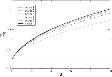
Figure 2: Ground state energy of the AHO as a function of $\mu$ to different perturbative orders, assuming $\hbar=m=\omega=1$.

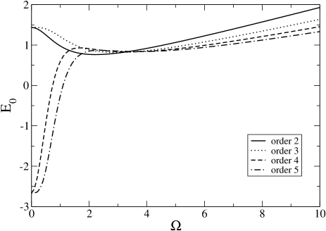
Figure 3: Energy of the AHO as a function of $\Omega$, at different perturbative orders ($\hbar=m=\omega=1$) and keeping $\mu$ fixed ($\mu=5$).

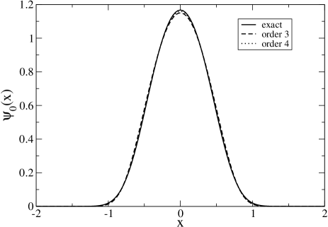
Figure 4: Wave function for the ground state of the anharmonic oscillator, assuming $m=\hbar=\omega=1$ and $\mu=200$. The solid line is the exact result whereas the dashed (dotted) line is the result obtained with our method to third (fourth) order.

In Fig. 3 we show the energy of the AHO as a function of the parameter $\Omega$, for $\mu=5$. The different curves correspond to different orders in perturbation theory (from second up to fifth order). We observe that the energy at different orders in the perturbative expansion develops local minima and maxima. By applying the PMS we select the extremum in which the energy is flatter, i. e. where the dependence upon $\Omega$ is smaller.

It should be remarked that the method works equally well for the wave function. Indeed, in Fig. 4 we plot the wave function of the ground state of the AHO. The solid line is the exact (numerical) result, whereas the dashed and dotted lines refer to the wave function obtained by applying our method to third and fourth order respectively. We see that it works extremely well, even for large values of $\mu$ ($\mu=200$). Although we have not imposed that the wave function be flat at the origin, we observe that the method naturally provides this result.

Finally, we would like to stress that, although we have displayed results up to a few orders in the perturbative expansion, it is very easy to push the calculation to any order, since the method only requires the solution of algebraic equations order by order.

We are currently working on the application of our method to the calculation of the excited states of the AHO, to more general anharmonic potentials and to the double-well potential.

- (1) T. Hatsuda, T. Kunihiro, and T. Tanaka, Phys. Rev. Lett. 78, 3229 (1997) [arXiv:hep-th/9612097].
- (2) C. M. Bender and L. M. A. Bettencourt, Phys. Rev. D 54, 7710 (1996) [arXiv:hep-th/9607074].
- (3) R. Guida, K. Konishi, and H. Suzuki, Ann. Phys. (N.Y.) 241, 152 (1995) [arXiv:hep-th/9407027].
- (4) W. Janke and H. Kleinert, Phys. Rev. Lett. 75, 2787 (1995).
- (5) A. Okopińska, Phys. Rev. D 35, 1835 (1987); A. Duncan and M. Moshe, Phys. Lett. B 215, 352 (1988).
- (6) M. P. Blencowe and A. P. Korte, Phys. Rev. B 56, 9422 (1997) [arXiv:cond-mat/9706260].
- (7) H. F. Jones, P. Parkin and D. Winder, Phys. Rev. D 63, 125013 (2001) [arXiv:hep-th/0008069].
- (8) J. L. Kneur, M. B. Pinto, and R. O. Ramos, arXiv:cond-mat/0207295.
- (9) J. L. Kneur, M. B. Pinto, and R. O. Ramos, Phys. Rev. Lett. 89, 210403 (2002) [arXiv:cond-mat/0207089].
- (10) G. Krein, D. P. Menezes, and M. B. Pinto, Phys. Lett. B 370, 5 (1996) [arXiv:nucl-th/9510059].
- (11) M. B. Pinto and R. O. Ramos, Phys. Rev. D 60, 105005 (1999) [arXiv:hep-ph/9903353].
- (12) P. Amore and A. Aranda, submitted to Phys. Lett. A [arXiv:math-ph/0303042].
- (13) P. Amore and A. Aranda, submitted to Phys. Rev. E [arXiv:math-ph/0303052].
- (14) P. M. Stevenson, Phys. Rev. D 23, 2916 (1981).
- (15) P. Amore, A. Aranda, and A. De Pace, work in progress.
- (16) W. Janke and H. Kleinert, Phys. Lett. A 206, 283 (1995) [arXiv:quant-ph/9502019].