Decoherence of the flux-based superconducting qubit in an integrated circuit environment

Abstract

Superconducting, flux-based qubits are promising candidates for the construction of a large scale quantum computer. We present an explicit quantum mechanical calculation of the coherent behavior of a flux based quantum bit in a noisy experimental environment such as an integrated circuit containing bias and control electronics. We show that non-thermal noise sources, such as bias current fluctuations and magnetic coupling to nearby active control circuits, will cause decoherence of a flux-based qubit on a timescale comparable to recent experimental coherence time measurements.

I INTRODUCTION

The possibility of observing quantum coherent behavior in macroscopic devices, such as superconducting circuits, was first suggested by A. J. Leggett in the mid 1980’s 1 . Since then, experimentalists have attempted to observe such behavior 2 ; 3 and, more recently, to extend the idea to a full scale quantum computer capable of executing quantum algorithms such as Shor’s algorithm 4 . Superconducting qubit types include charge qubits: created by a superposition of the number of electrons on a superconducting island 5 ; phase qubits: the superposition of energy states in a single Josephson junction 6 ; and flux qubits: the superposition of the quantity of flux threading a superconducting ring interrupted by a Josephson junction 7 . Quantum mechanical behavior has been verified in all three of these qubit systems, and experiments have shown that each system can be prepared in quantum superpositions. The coherence times which result from these environmental interactions, however, are far shorter than those predicted by current theories of open quantum systems.

Non-thermal sources of noise, such as fluctuations from room temperature laboratory control and measurement equipment and active circuit elements operating in the vicinity of the quantum device will contribute to the decoherence of the qubit in ways that are unique to different experimental configurations and methods. In this work we calculate the coherence time of a flux-based quantum bit exposed to classical noise sources consistent with those that would be found in an integrated circuit environment. We explicitly calculate the evolution of the qubit wavefunction under the influence of a Hamiltonian including environmental noise and infer decoherence times via an ensemble average of such calculations.

The future of solid state quantum computation will likely involve the integration of quantum bits onto a monolithic circuit also containing classical electronics used for quantum state preparation, manipulation and readout 4 ; 8 . For a large-scale quantum computer the classical control electronics will most likely be digital and be implemented in a well understood, robust technology such as superconducting rapid single flux quantum (RSFQ) technology. RSFQ logic is an integrated circuit family

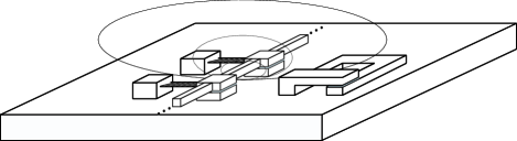
Figure 1: A RSFQ circuit (left) physically near and inductively coupled to a rf-SQUID qubit (right). The RSFQ circuit passes digital bits as quantized units of magnetic flux. The physical proximity of the active circuit will destroy the coherent behavior of the rf-SQUID qubit. The elliptical lines surrounding the RSFQ inductor are the field lines created by a passing data pulse.

that uses single flux quantum (SFQ) magnetic pulses as data bits. A diagram of a likely physical layout of an integrated circuit is illustrated in Fig. 1, where RSFQ digital circuitry is placed near by and inductively coupled to a rf-SQUID qubit. Unlike charge and phase based Josephson qubits, the flux based rf-SQUID qubit is inductively coupled to the environment making it susceptible to the effects of stray magnetic fields. The quantum dynamics of the rf-SQUID is exceedingly sensitive to the applied external magnetic field. The mutual inductance of the rf-SQUID qubit facilitates simple coupling procedures between qubits and classical circuitry, but also leaves the qubit vulnerable to unwanted coupling to active circuit elements integrated on the same chip. Although one clearly will attempt to shield the qubit from such stray fields these measures cannot be perfect. Furthermore, in order to be of any practical use, the flux qubits can not be completely isolated. Studies have been performed evaluating the effect of mutual inductive coupling in standard CMOS circuit technology 9 . Due to the robustness of digital logic, classical circuitry has a high level of immunity to these types of effects, contrary to quantum coherent technologies, which will be extremely sensitive to noise coupled through a mutual inductance.

Though quantum dynamics of the rf-SQUID have been verified, the macroscopic quantum coherent (MQC) oscillations of flux, predicted by A.J. Leggett 1 have not yet been directly observed due to the lack of sufficiently sensitive and fast means of measurement. By integrating the entire MQC experiment onto a monolithic circuit we believe it will be possible to create the necessary electronics to conduct the experiment. Furthermore, such chips used to perform the necessary experimental procedures can be used to explore decoherence mechanisms arising from qubit coupling to classical noise sources.

The calculation performed in the following sections models the decoherence of a rf-SQUID qubit integrated with active, classical circuitry. The effect of the classical circuits on the qubit is modeled by the inclusion of fluctuating terms in the Hamiltonian of the rf-SQUID. The classical sources of noise are characterized by Gaussian random variables with a finite bandwidth and predetermined power spectral density (PSD). The predicted qubit coherence times depend upon characteristics of the classical noise that may be measured experimentally.

II The Decoherence Calculation

Decoherence can most easily be defined as the deviation of the behavior of a quantum mechanical system from that predicted by the Schr dinger equation for the closed quantum system. Traditionally, decoherence is defined in the context of the density matrix ($\rho$) representation where loss of coherence in a quantum system is indicated by the suppression of the off-diagonal elements of the density matrix. In a given basis,

$$\rho(t)=\frac{1}{N}\sum_{i=1}^{N}|\psi_{i}(t)\rangle\langle\psi_{i}(t)|,$$ (1)

where $N$ is the number of individual systems composing the ensemble about which quantum statistics are being described and $|\psi_{i}(t)\rangle$ is the state of the $i^{th}$ system. When the off-diagonal elements of $\rho$ are completely suppressed evaluation of the Schr¨dinger equation for the closed system ceases to be an accurate predition of the evolution of the state $|\psi\rangle$ of the open system. Decoherence models have been created to predict the time scales on which non-deterministic degrees of freedom of the environment become entangled with the qubit thereby destroying the coherence of the quantum system 10 . There is a large body of work on the decoherence of a spin-1/2 system coupled to a reservoir of harmonic oscillators 11 ; 12 . To our knowledge, however, an explicit, time-dependent calculation of the evolution of a flux-based qubit including the effects of a noisy environment has not been completed.

Two distinguishable decoherence mechanisms contribute to the suppression of the off-diagonal elements of $\rho$. Relaxation is associated with an increase or reduction of the expectation value of the energy. Dephasing is an adiabatic process whereby the phase of the system wavefunction becomes randomized. Dephasing typically occurs on a much shorter timescale than relaxation 13 .

The Hamiltonian for the rf-SQUID, derived in 1 , is given by,

$$H=\frac{-\hbar^{2}}{2C}\frac{\partial^{2}}{\partial\Phi^{2}}+\frac{\left(\Phi-\Phi_{x}\right)^{2}}{2L}-\frac{I_{c}\Phi_{0}}{2\pi}\cos\left(\frac{2\pi\Phi}{\Phi_{0}}\right).$$ (2)

In this equation $C$ is the capacitance of the Josephson junction, $\Phi_{x}$ is the magnetic flux applied to the device externally and $L$ is the loop inductance. The independent variable, $\Phi$ is the flux threading the superconducting loop. The first term represents the kinetic energy of the SQUID, while the second and third terms constitute the potential energy of the superconducting inductor and Josephson junction, respectively.

The qubit potential has two independent degrees of freedom, the height of the barrier separating the two minima, and the relative depth of the two minima. The Hamiltonian can be rewritten in a form similar to that of a two-state system as,

$$H_{tss}=-\frac{\hbar\Delta}{2}\sigma_{x}+\frac{\epsilon}{2}\sigma_{z},$$ (3)

where $\Delta$ is the tunnelling matrix element, and $\epsilon$ is the difference in energy between the ground states of the two wells. The operators $\sigma_{x}$ and $\sigma_{z}$ are Pauli matrices. In principle these two degrees of freedom are separable, and can be considered independently. In a laboratory setting, however, they are subject to the same environmental influences and should be considered simultaneously when examining decoherence. The flux states of the system correspond to the eigenstates of $\sigma_{z}$. In this basis fluctuations in the barrier height are referred to as $\sigma_{x}$ fluctuations because they modulate the energy level spacing and fluctuations in the relative depths of the wells are called $\sigma_{z}$ fluctuations. When the flux bias deviates from $\Phi_{0}/2$ by greater than $10^{-4}\Phi_{0}$, the energy and flux basis states are nearly the same. However, when the system is flux biased at exactly $\Phi_{0}/2$ the energy bases are non-local in flux; there is finite probability of finding the flux in either well. Traditionally, $\sigma_{z}$ fluctuations are considered to be the most destructive to the coherence of a system. In a typical experiment[2], the single rf-SQUID junction is replaced by a double junction loop of small self-inductance. This added inductance will promote coupling between the environmental fluctuations and $\sigma_{x}$ degree of freedom in the system. The contribution to dephasing from $\sigma_{x}$ and $\sigma_{z}$ degrees of freedom will depend on the ratio of the self-inductances of the junction loop and SQUID loop, respectively. Reducing the junction loop inductance will allow $\sigma_{x}$ dephasing to be ignored.

As stated earlier, the calculation performed in this paper is an explicit solution of the time-dependant Schr dinger equation. Previous calculations of the decoherence of a rf-SQUID have focused on modeling the interaction of the environment as a continuous weak measurement 14 or by reducing the problem to a two-state system and using the spin-boson formalism 12 ; 15 . The shortcomings of these models are that they approximate the effect of a general environment on the system, but do not accurately reflect the dominant sources of noise in a circuit environment. For example, the spin-boson formalism reduces the qubit to a system with only two energy levels and models the interaction between the qubit and environment as bilateral, in that the state of the qubit affects the state of the environment. In an integrated circuit environment the back action of the qubit on the sources of the fluctuating fields is insignificant.

The illustration in Fig. 1 depicts an RSFQ integrated circuit, consisting of resistors and superconducting inductors and Josephson junctions near a rf-SQUID qubit. The magnetic data pulses that propagate through the RSFQ circuit will inductively couple flux to the qubit perturbing the otherwise constant external flux bias; it is necessary to determine the magnitude of these decoherence causing fluctuations. Stray magnetic flux coupled to the qubit from the RSFQ circuitry is determined by the magnitude of the current pulses in nearby RSFQ circuits and the mutual inductance ($M$) between the circuits and qubit. A typical estimate for $M$ when the circuit and qubit are $20\mu m$ apart is on the order of $10fH$. A SFQ data pulse passing through a superconducting inductor of typical size in RSFQ circuits has a peak amplitude of approximately $150\mu A$ and a duration of $2-4ps$. With these parameters the excess flux coupled to the qubit is $720\mu\Phi_{0}$. An analysis of the decoherence effects in such a situation follows.

The effect of a large number of nearby RSFQ circuits, each passing SFQ pulses at seemingly random times from the point of view of the qubit, may be represented by introducing a random component to the flux in the vicinity of the qubit. Thus, our calculation was performed by introducing noise terms directly into the Hamiltonian, Eq. 2, and then solving the time-dependant Schr dinger equation with the random Hamiltonian. The rf-SQUID can be perturbed by the flux environment in two ways: the external flux bias applied to the qubit can deviate from $\Phi_{0}/2$, or magnetic flux can couple to the Josephson junction thereby changing the effective $I_{c}$. As shown earlier the influence of the fluctuations of the applied flux bias, $\sigma_{z}$ noise, dominates the effect of qubit junction critical current fluctuations, the $\sigma_{x}$ noise. Therefore a random term was added to in the Hamiltonian and the evolution of the qubit was computed. The initial wavefunction, $|\Psi_{0}\rangle$, used in the calculation was determined by the ground state of the system with slightly less than $\Phi_{0}/2$ applied flux. At milliKelvin temperatures the system will completely relax to this state. $|\Psi_{0}\rangle$ is then projected onto the basis functions of the symmetric double well potential. The state of the system is nearly a pure superposition of the ground and first excited state of the symmetric potential. There are, however, excitations of higher lying states that are small but nonetheless included in the calculation.

The time evolution of the system is determined using a time varying propagator operating on the wavefunction,

$$|\psi_{m}(t+\Delta t)\rangle=exp(iH_{m}(t+\Delta t)\Delta t)|\psi_{m}(t)\rangle,$$ (4)

where $H_{m}(t+\Delta t)$ is the Hamiltonian of the system with $\Phi_{x}(t+\Delta t)$ and $I_{c}(t+\Delta t)$ ; we also chose $\Delta t$ to be $100ps$, much shorter than the period of the MQC oscillations. At each time step the wave function $|\psi_{m}(t)\rangle$ is projected onto the basis states of the new Hamiltonian $H_{m}(t+\Delta t)$, which are determined before the calculation and stored in a look up table, and then evolved through time $\Delta t$ to produce the new wavefunction, $|\psi_{m}(t+\Delta t)\rangle$. The result for short time-scales is a randomization of the phase of the coherent oscillations of the flux. On a longer time-scales the populations of the energy levels will deviate from those of $|\Psi_{0}\rangle$. Since the loss of phase coherence occurs on a shorter time-scale that is the dominant form of decoherence and thus will be the subject of this work.

In order to calculate the dephasing time of the MQC oscillations in the fluctuating potential the simulation described above is repeated many times, and the separate results are averaged as shown in Eq. 1. An experimental technique similar to the one described here was used in 16 to measure the phase stability of classical oscillators. For our calculation we used $N=50$. For each trial the phase of the oscillations becomes unpredictable after some period of time. Thus averaging over a large number of random phases leads to the vanishing of the off-diagonal elements of the density matrix in Eq. 1.

A set of $N$ evolutions was performed and summed for each value of

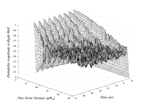
Figure 2: A surface plot of the data obtained from the calculation of decoherence of the rf-SQUID qubit. As the variance of the flux noise influencing the qubit is increased, the coherent oscillations of flux last for shorter amounts of time.

flux noise variance, and the results are plotted in the surface plot of Fig. 2. The bandwidth of the noise in Fig. 2 is $4GHz$. To quantify the dephasing time resulting from each value of flux noise variance, the damped sinusoid resulting from the set of N evolutions was fit to a function of the form,

$$P(t)=exp(-D_{\phi}t)cos(\omega_{0}t+\pi),$$ (5)

where $\omega_{0}$ is the resonant frequency of the tunnelling flux, which is also equal to the energy splitting between the ground and first excited states. The value of the dephasing time constant, $D_{\phi}$, for each value of flux noise variance was

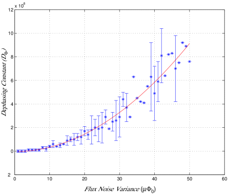
Figure 3: A plot of the dephasing rate as a function of flux noise variance. The bandwidth of the noise signal used for this data is $4GHz$. Error bars are provided for selected data points indicating the confidence of the fit.

determined using a least squares fit to the data obtained in Fig. 2. Fig. 3 shows the plot of $D_{\phi}$ as a function of the flux noise variance, $\sigma_{\phi}$, applied to the qubit. From the graph in Fig. 3 the relation between $D_{\phi}$ and the variance is $D_{\phi}=3.63\cdot 10^{-4}\left(\sigma_{\phi}\right)^{2}$ (1/ns), where $\sigma_{\phi}$ is in units of $\mu\Phi_{0}$. Since $\sigma_{\phi}^{2}=\int_{-\infty}^{\infty}S_{\Phi}(\omega)d\omega$, $D_{\phi}$ is linearly proportional to the amplitude of the power spectral density of the environmental flux noise at a given bandwidth. Fig. 2 shows that if the flux noise variance is increased above approximately $10\mu\Phi_{0}$ , then the coherence of the qubit lasts less than $20ns$. From the physical scenario described above, it is evident that $M$ must be reduced by at least two orders of magnitude, to below $.1fH$, in order for the excess flux to be reduced to these levels and for acceptable coherence times to be achieved.

An analysis was also performed to measure the dependence of $D_{\phi}$ on the bandwidth of the noise signal. It was seen that if the noise is bandlimited to a cutoff frequency, $\omega_{c}$, below $\omega_{0}$, then $D_{\phi}$ varies approximately linearly with the noise bandwidth. If $\omega_{c}\geq\omega_{0}$, $D_{\phi}$ is nearly independent of the bandwidth of the noise signal. When the noise is bandlimited so that $\omega_{c}\leq\omega_{0}$ the frequency of the oscillations is no longer $\omega_{0}$ due to the fact that on the timescales in question noise bandlimited below $\omega_{0}$ can no longer be considered white, and $\overline{\Phi_{x}}\neq\frac{\Phi_{0}}{2}$. This yields a noticeable increase in the coherent tunnelling frequency of the system. At noise frequencies greater than $\omega_{0}$ the noise can be considered white and $\overline{\Phi_{x}}=\frac{\Phi_{0}}{2}$ over the 35 ns time scale of the simulation. At large noise frequencies the dephasing rate, $D_{\phi}$, is dependent primarily on the variance of the flux noise and nearly independent of the bandwidth of the noise. In an integrated circuit environment, especially one operating at GHz speeds, the bandwidth of the noise created by the circuitry will certainly exceed that of $\omega_{0}$, which in this case is approximately 280 MHz.

III Conclusions

The ultimate goal of integrating classical electronics with coherent quantum circuitry is to efficiently prepare and manipulate the coherent states of the qubits. This will require that classical circuitry, such as RSFQ, be placed in close proximity to the quantum coherent bits in order to provide the necessary interaction, which in this case is inductive. Unwanted interactions between unintentionally coupled classical circuitry and qubits will no doubt exist and it must be determined what effect that will have on the coherence time of the qubits. We have calculated that for current RSFQ technology there is a threshold value for the mutual inductance between RSFQ circuitry and a qubit of approximately $0.1fH$ below which qubit coherence times may persist for longer than $20ns$.

We have used an explicit formulation of the Hamiltonian of the rf-SQUID in a noisy environment in order to determine a realistic value for the dephasing time in an integrated circuit environment. Moreover, the parameter that accounts for the loss of coherence in this model, the flux noise variance, is easily measured by incorporating a dc-SQUID magnetometer in the vicinity of the qubit. The approach presented here for estimating the coherence time of a rf-SQUID qubit is not intended as a general model of decoherence for two-state systems. Rather it provides an explicit model from which coherence times of rf-SQUID qubits may be estimated based upon experimentally measurable quantities. Models such as this one coupled with measurements of the flux noise at the location of the qubit will help quantum computer architects design large scale computers capable of executing the algorithms for which they were originally intended.

IV AKNOWLEDGEMENTS

Supported in part by AFOSR grant F49620-01-1-0457 funded under the Department of Defense University Research Initiative on Nanotechnology (DURINT) program and by the ARDA. J.L.H. is supported by a NASA GSRP fellowship.

References

- (1) A.J. Legget, in Quantum Mechanics at the Macroscopic Level, edited by G. Grinstein and G. Mazenko, Directions in Condensed Matter Physics Vol. 1 (1986).
- (2) J. Friedman et al., Nature 406, 43 (2000).
- (3) C. van der Wal, Science 290, 773 (2000).
- (4) M. Bocko, A. Herr and M. Feldman, IEEE Trans. On Applied Superconductivity 7, 3638 (1997).
- (5) J. Tsai, Y. Nakamura and Y. Pashkin, Physica C 375, 1 (2001).
- (6) Y. Yu et al., Science 296, 889 (2002).
- (7) J.E. Mooij et al., Science 285, 1036 (1999).
- (8) B.E. Kane, Progress of Physics 48, 1023 (2000).
- (9) M.H. Chowdhury et al., 2002 IEEE International Symposium on Circuits and Systems, (2002).
- (10) W. Zurek, Physics Today 44, 10 (1991).
- (11) M. Grifoni, E. Paladino and U. Weiss, Eur. Phys. J. B 10, 719 (1999).
- (12) U. Weiss, H. Grabert and S. Linkwitz, J. of Low Temp. Phys. 68, 213 (1987).
- (13) M. Governale, M. Grifoni and G. Schön, Chemical Physics 268, 273 (2001).
- (14) L. Viola, T. Onofrio and T. Calarco, Phys. Lett. A 229, 23 (1997).
- (15) A.J. Leggett et al., Rev. Mod. Phys. 67, 725 (1995).
- (16) D. Ham and A. Hajimiri, (to appear) IEEE J. of Solid State Circuits 38(3), (2003).