Quantum Computing and Error Correction

Abstract

The main ideas of quantum error correction are introduced. These are encoding, extraction of syndromes, error operators, and code construction. It is shown that general noise and relaxation of a set of 2-state quantum systems can always be understood as a combination of Pauli operators acting on the system. Each quantum error correcting code allows a subset of these errors to be corrected. In many situations the noise is such that the remaining uncorrectable errors are unlikely to arise, and hence quantum error correction has a high probability of success. In order to achieve the best noise tolerance in the presence of noise and imprecision throughout the computer, a hierarchical construction of a quantum computer is proposed.

1 Introduction

Quantum error correction (QEC) is one of the basic components of quantum information theory. It arises from the union of quantum mechanics and classical information theory, and leads to some powerful and surprising possibilities in the quantum context. For example, we may use a quantum error correcting code to allow us to store a general, unknown state of a two-state system in a set of five two-state systems (eg two-level atoms), in such a way that if any unknown change (arbitrarily large and including the case of relaxation) should occur in the state of any one atom, then it is still possible to recover the originally stored state precisely: the seemingly large perturbation had no effect at all on the stored information.

QEC is by now sufficiently well established that it has chapters devoted to it in text books, for example [1, 2, 3]. Nevertheless, an introduction to the ideas is still useful for people new to the subject, so much of the discussion here will be devoted to this. I will then discuss recent research in section 7.

QEC may be considered to consist of two separate parts. The first part is the theory of quantum error correcting codes, syndromes and quantum error operators. This is essentially a collection of physical insights and mathematical ideas which follow directly from the principles of quantum mechanics and are uncontroversial. The second part is the physics of noise, which must include the theory of how an open quantum system interacts with its environment. The success of QEC methods in practice will depend on our having the correct understanding of noise in open quantum systems. There is still some controversy over which methods can be correctly applied when we are considering large-scale systems such as a ‘classical’ environment, but the success of QEC is found not to depend on special pleading in this area. Nevertheless, it is necessary to be careful to examine what assumptions are required, so the presentation here will focus on this, particularly in sections 4 and 6.

2 Background

The first quantum error correcting codes were discovered independently by Shor [4] and Steane [5]. Shor proved that 9 qubits could be used to protect a single qubit against general errors, while Steane described a general code construction whose simplest example does the same job using 7 qubits (see section 5.1). A general theory of quantum error correction dates from subsequent papers of Calderbank and Shor [6] and Steane [7] in which general code constructions, existence proofs, and correction methods were given. Knill and Laflamme [8] and Bennett et. al. [9] provided a more general theoretical framework, describing requirements for quantum error correcting codes, and measures of the fidelity of corrected states.

The important concept of the stabilizer (section 5.1) is due to Gottesman [10] and independently Calderbank et. al. [11]; this yielded many useful insights into the subject, and permitted many new codes to be discovered [10, 11, 12]. Stabilizer methods will probably make a valuable contribution to other areas in quantum information physics. The idea of recursively encoding and encoding again was explored by several authors [13, 14, 15], this uses more quantum resources in a hierarchical way, to permit communication over arbitrarily long times or distances. Van Enk et. al. [16, 17] have discussed quantum communication over noisy channels using a realistic model of trapped atoms and high-quality optical cavities, and recursive techniques for systems in which two-way classical communication is possible were described by Briegel et al. [18].

Quantum error correction is discussed in reviews of quantum information theory, see for example [19, 20].

3 Three bit code

We will begin by analysing in detail the workings of the most simple quantum error correcting code. Exactly what is meant by a quantum error correcting code will become apparent.

Suppose a source A wishes transmit quantum information via a noisy communication channel to a receiver B. Obviously the channel must be noisy in practice since no channel is perfectly noise-free. However, in order to do better than merely sending quantum bits down the channel, we must know something about the noise. For this introductory section, the following properties will be assumed: the noise acts on each qubit independently, and for a given qubit has an effect chosen at random between leaving the qubit’s state unchanged (probability $1-p$) and applying a Pauli $\sigma_{x}$ operator (probability $p<1/2$). This is a very artificial type of noise, but once we can correct it, we will find that our correction can also offer useful results for much more realistic types of noise.

Figure 1: Example of quantum error correction which illustrates the main features. A single qubit is encoded into three, and these are sent down the noisy channel. The receiver introduces further qubits (the ancilla) and uses them to extract a syndrome by applying controlled-not gates and then measuring the ancilla bits. The received state can then be corrected. Finally, the single qubit of information may be re-extracted (decoded) from the three.

The simplest quantum error correction method is summarised in fig. 1. We adopt the convention of calling the source Alice and the receiver Bob. The state of any qubit which Alice wishes to transmit can be written without loss of generality $a\left|{0}\right>+b\left|{1}\right>$. Alice prepares two further qubits in the state $\left|{0}\right>$, so the initial state of all three is $a\left|{000}\right>+b\left|{100}\right>$. Alice now operates a controlled-not gate from the first qubit to the second, producing $a\left|{000}\right>+b\left|{110}\right>$, followed by a controlled-not gate from the first qubit to the third, producing $a\left|{000}\right>+b\left|{111}\right>$. Finally, Alice sends all three qubits down the channel.

The states $\left|{000}\right>$ and $\left|{111}\right>$ are called quantum codewords. Only codewords, or superpositions of them, are sent by Alice.

Bob receives the three qubits, but they have been acted on by the noise in the channel. Their state is one of the following:

$$\begin{array}[]{ll}\mbox{state}&\mbox{probability}\\ a\left|{000}\right>+b\left|{111}\right>&(1-p)^{3}\\ a\left|{100}\right>+b\left|{011}\right>&p(1-p)^{2}\\ a\left|{010}\right>+b\left|{101}\right>&p(1-p)^{2}\\ a\left|{001}\right>+b\left|{110}\right>&p(1-p)^{2}\\ a\left|{110}\right>+b\left|{001}\right>&p^{2}(1-p)\\ a\left|{101}\right>+b\left|{010}\right>&p^{2}(1-p)\\ a\left|{011}\right>+b\left|{100}\right>&p^{2}(1-p)\\ a\left|{111}\right>+b\left|{000}\right>&p^{3}\end{array}$$ (10)

Bob now introduces two more qubits of his own, prepared in the state $\left|{00}\right>$. This extra pair of qubits, referred to as an ancilla, is not strictly necessary, but makes error correction easier to understand and becomes necessary when fault-tolerant methods are needed. Bob uses the ancilla to gather information about the noise. He first carries out controlled-nots from the first and second received qubits to the first ancilla qubit, then from the first and third received qubits to the second ancilla bit. The total state of all five qubits is now

$$\begin{array}[]{cc}\mbox{state}&\mbox{probability}\\ (a\left|{000}\right>+b\left|{111}\right>)\left|{00}\right>&(1-p)^{3}\\ (a\left|{100}\right>+b\left|{011}\right>)\left|{11}\right>&p(1-p)^{2}\\ (a\left|{010}\right>+b\left|{101}\right>)\left|{10}\right>&p(1-p)^{2}\\ (a\left|{001}\right>+b\left|{110}\right>)\left|{01}\right>&p(1-p)^{2}\\ (a\left|{110}\right>+b\left|{001}\right>)\left|{01}\right>&p^{2}(1-p)\\ (a\left|{101}\right>+b\left|{010}\right>)\left|{10}\right>&p^{2}(1-p)\\ (a\left|{011}\right>+b\left|{100}\right>)\left|{11}\right>&p^{2}(1-p)\\ (a\left|{111}\right>+b\left|{000}\right>)\left|{00}\right>&p^{3}\end{array}$$ (20)

Bob measures the two ancilla bits in the basis $\{\left|{0}\right>,\left|{1}\right>\}$. This gives him two classical bits of information. This information is called the error syndrome, since it helps to diagnose the errors in the received qubits. Bob’s next action is as follows:

measured syndrome             action 00 do nothing 01 apply $$\sigma_{x} \sigma_{x} \sigma_{x}$$ to third qubit 10 apply to second qubit 11 apply to first qubit

Suppose for example that Bob’s measurements give $10$ (i.e. the ancilla state is projected onto $\left|{10}\right>$). Examining eq. (20), we see that the state of the received qubits must be either $a\left|{010}\right>+b\left|{101}\right>$ (probability $p(1-p)^{2}$) or $a\left|{101}\right>+b\left|{010}\right>$ (probability $p^{2}(1-p)$). Since the former is more likely, Bob corrects the state by applying a Pauli $\sigma_{x}$ operator to the second qubit. He thus obtains either $a\left|{000}\right>+b\left|{111}\right>$ (most likely) or $a\left|{111}\right>+b\left|{000}\right>$. Finally, to extract the qubit which Alice sent, Bob applies controlled-not from the first qubit to the second and third, obtaining either $(a\left|{0}\right>+b\left|{1}\right>)\left|{00}\right>$ or $(a\left|{1}\right>+b\left|{0}\right>)\left|{00}\right>$. Therefore Bob has either the exact qubit sent by Alice, or Alice’s qubit operated on by $\sigma_{x}$. Bob does not know which he has, but the important point is that the method has a probability of success greater than $1-p$. The correction is designed to succeed whenever either no or just one qubit is corrupted by the channel, which are the most likely possibilities. The failure probability is the probability that at least two qubits are corrupted by the channel, which is $3p^{2}(1-p)+p^{3}=3p^{2}-2p^{3}$, i.e. less than $p$ (as long as $p<1/2$).

To summarise, Alice communicates a single general qubit by expressing its state as a joint state of three qubits, which are then sent to Bob. Bob first applies error correction, then extracts a single qubit state. The probability that he fails to obtain Alice’s original state is $O(p^{2})$, whereas it would have been $O(p)$ if no error correction method had been used. We will see later that with more qubits the same basic ideas lead to much more powerful noise suppression, but it is worth noting that we already have quite an impressive result: by using just three times as many qubits, we reduce the error probability by a factor $\sim 1/3p$, i.e. a factor $\sim\!30$ for $p=0.01$, $\sim\!300$ for $p=0.001$, and so on.

3.1 Phase errors

The channel we just considered was rather artificial. However, it is closely related to a more realistic type of channel: one which generates random rotations of the qubits about the $z$ axis. Such a rotation is given by the operator

$$P(\epsilon\phi)=\left(\!\!\!\!\begin{array}[]{cc}e^{i\epsilon\phi}&0\\ 0&e^{-i\epsilon\phi}\end{array}\!\!\!\!\right)\equiv\cos(\epsilon\phi)I+i\sin(\epsilon\phi)\sigma_{z}$$ (21)

where $I$ is the identity, $\epsilon$ is a fixed quantity indicating the typical size of the rotations, and $0<\phi<2\pi$ is a random angle. We may understand such an error as a combination of no error ($I$) and a phase flip error ($\sigma_{z}$). We can deal with this situation by using exactly the same quantum error correcting code as before, only now at either end of the channel we apply to each qubit the Hadamard rotation

$$H\equiv\frac{1}{\sqrt{2}}\left(\begin{array}[]{cc}1&1\\ 1&-1\end{array}\right)$$

The combined effect of phase error and these Hadamard rotations is

$$HPH=\cos(\epsilon\phi)I+i\sin(\epsilon\phi)\sigma_{x}$$ (22)

which is easy to derive using $HH=I$ and $H\sigma_{z}H=\sigma_{x}$.

We now have a situation just like that considered in the previous section, only instead of a $\sigma_{x}$ ‘bit flip’ being applied randomly with probability $p$ to each qubit, every qubit certainly experiences an error which is a combination of the identity and $\sigma_{x}$. When we put this type of error through the analysis of the correction network shown in figure 1, modeling the measurements on the ancilla qubits as standard Von-Neumann projective measurements, the outcome is exactly as before, with the quantity $p$ equal to the average weight of the terms in the quantum state which have single bit-flip errors (before correction). This average is over the random variable $\phi$, thus $p=\left<\sin^{2}\epsilon\phi\right>\simeq(2\pi\epsilon)^{2}/3$ for $\epsilon\ll 1$, where we have considered the worst case, in which the states being transmitted are taken to orthogonal states by the action of $\sigma_{z}$. A complete calculation of the 3-qubit system, with the random rotations and the syndrome measurement described, confirms that the fidelity of the final corrected state is $f=1-3p^{2}$ for small $p$, in agreement with the results of the previous section.

3.2 Projective errors

It is a familiar feature of quantum mechanics that a set of particles where each is in an equal superposition of two states $(\left|{0}\right>+\exp(i\phi)\left|{1}\right>)/\sqrt{2}$, with the relative phase $\phi$ of the two terms random, is indistinguishable from a statistical mixture, i.e. a set of particles where each is either in the state $\left|{0}\right>$ or in $\left|{1}\right>$, randomly. This follows immediately from the fact that these two cases have the same density matrix. With this in mind, it should not be surprising that another type of error which the three-bit code can correct is an error consisting of a projection of the qubit onto the $\left|{0}\right>,\left|{1}\right>$ basis. To be specific, imagine the channel acts as follows: for each qubit passing through, either no change occurs (probability $1-2p$) or a projection onto the $\left|{0}\right>,\left|{1}\right>$ basis occurs (probability $2p$). The projection $\left|{0}\right>\left<{0}\right|=(I+\sigma_{z})/2$ and $\left|{1}\right>\left<{1}\right|=(I-\sigma_{z})/2$. Such errors are identical to phase errors (equation(21)), except for the absence of the factor $i$ before the $\sigma_{z}$ term. However, this factor does not affect the argument, and once again the analysis in equation (20) applies (once we have used the Hadamard ‘trick’ to convert phase errors to bit-flip errors) in the limit of small $p$. Note that we define $p$ in terms of the effect of the noise on the state: it is not the probability that a projection occurs, but the probability that a $\sigma_{z}$ error is produced in the state of any single qubit when quantum codewords are sent down the channel.

Another way of modeling projective errors is to consider that the projected qubit is first coupled to some other system, and then we ignore the state of the other system. Let such another system have, among its possible states, two states $\left|{\alpha}\right>_{e}$ and $\left|{\beta}\right>_{e}$ which are close to one another, $\left<{\alpha}\right.\left|{\beta}\right>=1-\epsilon$. The error consists in the following coupling between qubit and extra system:

$$\left(a\left|{0}\right>+b\left|{1}\right>\right)\left|{\alpha}\right>_{e}\rightarrow a\left|{0}\right>\left|{\alpha}\right>_{e}+b\left|{1}\right>\left|{\beta}\right>_{e}$$ (23)

this is an entanglement between the qubit and the extra system. A useful insight is to express the entangled state in the following way:

$$a\left|{0}\right>\left|{\alpha}\right>+b\left|{1}\right>\left|{\beta}\right>\equiv\frac{1}{\sqrt{2}}\left[\left(a\left|{0}\right>+b\left|{1}\right>\right)\left|{+}\right>_{e}+\left(a\left|{0}\right>-b\left|{1}\right>\right)\left|{-}\right>_{e}\right]$$ (24)

where $\left|{\pm}\right>_{e}=(\left|{\alpha}\right>_{e}\pm\left|{\beta}\right>_{e})/\sqrt{2}$. Hence the error on the qubit is seen to be a combination of identity and $\sigma_{z}$, and is correctable as before. The probability that the $\sigma_{z}$ error is produced is calculated by finding the weights of the different possibilities in equation (20) after the tracing over the extra system. We thus obtain $p=(1-{\rm Re}(\left<{\alpha}\right.\left|{\beta}\right>))^{2}/2=\epsilon^{2}/2$.

4 Most general possible error, digitization of noise

The most general possible error that a qubit can undergo is a general combination of the ones we have listed, that is, general rotations in the two-dimensional Hilbert space, combined with a possible projection onto any axis. In what follows we will model a projection by using the method just outlined, in which the qubit is entangled with another system, and the error consists in the fact that the entangling process can not be undone, because the other system is not under our control. In QEC it has become standard practice to refer to coupling to ‘the environment’ in this way. It might seem that this depends on modeling the environment as if it is a quantum system with unitary evolution, but in fact the technique is only a mathematical convenience for dealing with projections. If one is uncomfortable with writing down quantum states of the environment, then one should return to the language of projection, and the conclusions concerning the efficacy of QEC will remain unchanged.

With these considerations in mind, we now come to one of the basic insights of QEC: a completely arbitrary change in a general state $\left|{\phi}\right>$ of a qubit can be written

$$\left|{\phi}\right>\left|{\psi_{0}}\right>_{e}\rightarrow\sum_{i=\{I,x,y,z\}}\left(\sigma_{i}\left|{\phi}\right>\right)\left|{\psi_{i}}\right>_{e}$$ (25)

where we have written $I=\sigma_{I}$ and the second system with states $\left|{\psi_{i}}\right>_{e}$ (typically called ‘states of the environment’) is introduced simply to allow us to write using the language of kets a general change in the density matrix of the qubit. This density matrix of the qubit is the reduced density matrix of the pair of systems, after tracing over the second system. We can thus reproduce arbitrary changes in the density matrix of the qubit as long as we allow the states $\left|{\psi_{i}}\right>_{e}$ to be unconstrained, that is, they are not necessarily either normalised or orthogonal.

Generalising this insight, we find that any transformation of the state of a set of qubits can be expressed

$$\left|{\phi}\right>\left|{\psi_{0}}\right>_{e}\rightarrow\sum_{i}\left(E_{i}\left|{\phi}\right>\right)\left|{\psi_{i}}\right>_{e}$$ (26)

where each ‘error operator’ $E_{i}$ is a tensor product of Pauli operators acting on the qubits, $\left|{\phi}\right>$ is the initial state of the qubits, and $\left|{\psi_{i}}\right>_{e}$ are states of a second system, not necessarily orthogonal or normalised.

We thus express general noise and/or decoherence in terms of Pauli operators $\sigma_{x}$, $\sigma_{y}$, $\sigma_{z}$ acting on the qubits. These will be written $X\equiv\sigma_{x}$, $Z\equiv\sigma_{z}$, $Y\equiv-i\sigma_{y}=XZ$. The remarkable fact embodied by (26) is that arbitrary changes, which form a continuous set, can be ‘digitized’ by expressing them as a weighted sum of discrete errors. This arises from the fact that the Pauli matrices with the identity form a complete set.

To write tensor products of Pauli matrices acting on $n$ qubits, we introduce the notation $X_{u}Z_{v}$ where $u$ and $v$ are $n$-bit binary vectors. The non-zero coordinates of $u$ and $v$ indicate where $X$ and $Z$ operators appear in the product. For example,

$$X\otimes I\otimes Z\otimes Y\otimes X\equiv X_{10011}Z_{00110}.$$ (27)

The weight of an error operator is the number of terms in the tensor product which are not the identity, this is 4 in the example just given.

Error correction is a process which takes a state such as $E_{i}\left|{\phi}\right>$ to $\left|{\phi}\right>$. Correction of $X$ errors takes $X_{u}Z_{v}\left|{\phi}\right>$ to $Z_{v}\left|{\phi}\right>$; correction of $Z$ errors takes $X_{u}Z_{v}\left|{\phi}\right>$ to $X_{v}\left|{\phi}\right>$. Putting all this together, we discover the highly significant fact that to correct the most general possible noise (eq. (26)), it is sufficient to correct just $X$ and $Z$ errors. See eq. (28) and following for a proof. It may look like we are only correcting unitary ‘bit flip’ and ‘phase flip’ rotations, but this is a false impression: actually we will correct everything, including non-unitary relaxation processes!

5 Correction of general errors

A general quantum error correcting code will be an orthornormal set of $n$-qubit states (quantum codewords) which allow correction of all members of a set $S=\{E_{i}\}$ of correctable errors. We are usually interested in the case where the correctable errors include all errors (including $X$, $Y$ or $Z$ and combinations thereof for different qubits) of weight up to some maximum $w$. Such a code is called a $w$-error correcting code. It can be shown that such a code allows perfect correction of any change in the $n$-qubit quantum state which affects at most $w$ qubits [7, 6]. The correction method is comparable to that shown in figure 1 for the simple 3-bit code, where first a syndrome is extracted, and then the state is corrected accordingly.

The main steps in the proof of this claim are as follows. Let $\left|{\phi}\right>_{L}$ be a state consisting of a general superposition of codewords of some QEC code. A general noise process (26) will then produce the state

$$\sum_{i}\left(E_{i}\left|{\phi}\right>_{L}\right)\left|{\psi_{i}}\right>_{e}$$ (28)

The syndrome extraction can be done most simply by attaching an $n-k$ qubit ancilla $a$ to the system (this is not the only method, but is convenient), and storing in it the parity checks which are satisfied by the quantum codewords, using controlled-not and Hadamard operations. Another way of saying the same thing is that we store into the ancilla the eigenvalues of a set of simultaneously commuting operators (the stabilizer) acting on the noisy state. The quantum codewords themselves are all simultaneous eigenstates with eigenvalue 1 of all the operators in the stabilizer, so such a process does not have any effect on a general noise-free state. In the case of a noisy state, the effect is to couple system and environment with the ancilla as follows:

$$\left|{0}\right>_{a}\sum_{i}\left(E_{i}\left|{\phi}\right>_{L}\right)\left|{\psi_{i}}\right>_{e}\rightarrow\sum_{i}\left|{s_{i}}\right>_{a}\left(E_{i}\left|{\phi}\right>_{L}\right)\left|{\psi_{i}}\right>_{e}.$$ (29)

The $s_{i}$ are $(n-k)$-bit binary strings, the syndromes. A projective measurement of the ancilla will collapse the sum to a single syndrome taken at random: $\left|{s_{i}}\right>_{a}\left(E_{i}\left|{\phi}\right>_{L}\right)\left|{\psi_{i}}\right>_{e}$, and will yield $s_{i}$ as the measurement result. To keep the argument clear, we have assumed that every $E_{i}$ will have a different syndrome. This assumption will be dropped in a moment. Since there is only one $E_{i}$ with the syndrome we have measured, we can deduce the operator $E_{i}^{-1}$ which should now be applied to correct the error. The resulting state is $\left|{s_{i}}\right>_{a}\left|{\phi}\right>_{L}\left|{\psi_{i}}\right>_{e}$, and now we can ignore the state of environment and ancilla without affecting the system, since they are in a product state. The system is therefore “magically” disentangled from its environment, and perfectly restored to $\left|{\phi}\right>_{L}$!

This remarkable process can be understood as first forcing the general noisy state to ‘choose’ among a discrete set of errors, via a projective measurement, and then reversing the particular discrete error ‘chosen’ using the fact that the measurement result tells us which one it was. Alternatively, the correction can be accomplished by a unitary evolution consisting of controlled gates with ancilla as control, system as target, effectively transferring the noise (including entanglement with the environment) from system to ancilla.

In general the true situation is that more than one error operator has the same syndrome, just as in equation (20). If two error operators $E_{1}$, $E_{2}$ have the same syndrome $s$ for a given QEC code, then upon obtaining $s$ in the syndrome extraction we apply to the qubits the inverse of whichever of $E_{1}$ and $E_{2}$ was most likely to have been produced by the noise process. The other error operator is then an uncorrectable error. This will be considered further in section 6.

5.1 Example codes

The above abstract treatment is clarified by some specific examples. In section 3 we considered a simple example where either an $X$ error or a $Z$ error (on any single qubit) was correctable. The most important generalisation is to the case of a code which allows both an $X$ error and a $Z$ error to be corrected. We will then further generalise to the case where errors affecting more than one qubit are correctable.

We have already noted that $HZH=X$ and this means that if the set of states (quantum error correcting code) $\{\left|{u}\right>\}$ are to be correctable for $X$ and $Z$ errors, it is sufficient and necessary that $\{\left|{u}\right>\}$ and $\{{\bf H}\left|{u}\right>\}$ both be correctable for $X$ errors, where ${\bf H}=H\otimes H\otimes H\cdots\otimes H$ signifies the Hadamard rotation applied to all $n$ qubits. This was how the first general class of QEC codes was discovered [7, 6]. A general formalism in which such ideas can be handled succinctly has been developed by Gottesman [10] and Calderbank et al. [21]. The simplest (though not the shortest) single-error correcting code is the 7-bit code having two codewords given by

$$\left|{0}\right>_{L} = \left|{0000000}\right>+\left|{1010101}\right>+\left|{0110011}\right>+\left|{1100110}\right>$$

$$\!\!\!\!\!\!+\left|{0001111}\right>+\left|{1011010}\right>+\left|{0111100}\right>+\left|{1101001}\right>,$$

$$\left|{1}\right>_{L} = X_{1111111}\left|{0}\right>_{L}.$$ (30)

This code is constructed by combining two classical error correcting codes: the states occurring in $\left|{0}\right>_{L}$ are all the members of a classical error correcting code $C$ which has minimum distance 4, and the states occurring in ${\bf H}\left|{0}\right>_{L}$ are all the members of another classical error correcting code $C^{\perp}$ (the dual of $C$) which has minimum distance 3 and which contains $C$. Furthermore, any superposition of $\left|{0}\right>_{L}$ and $\left|{1}\right>_{L}$ only involves members of $C^{\perp}$, and this is also true for any superposition of ${\bf H}\left|{0}\right>_{L}$ and ${\bf H}\left|{1}\right>_{L}$. It is not my purpose to present this code construction fully, this may be found in the references given in the introductory sections above. The aim is to give enough information here to enable an understanding of the main themes to be gained.

I referred just now to the concept of ‘minimum distance’. For a set of binary words, the minimum distance is the minimum number of bits which must be flipped to convert one binary word in the set into another in the set. A classical error correcting code of distance $d$ can correct any set of bit flips as long as they affect no more than $(d-1)/2$ bits. In the quantum case it can be shown that codes can be constructed which allow correction of any error operator $E$ of weight less than or equal to $(d-1)/2$, where $d$ is now the minimum distance of the quantum code.

The code given by equation (30) has distance $3$ and is therefore a single-error-correcting quantum code. Since there are two orthogonal states in the code, only a single qubit of information can be stored in the 7 qubits employed. These parameters are summarised by the notation $[[n,k,d]]=[[7,1,3]]$. The code construction methods are now quite advanced. Infinite sets of codes of given distance are known, as well as a large set of quite powerful codes [21, 12]. Some parameters of known codes include, for example, $[[5,1,3]]$, $[[8,3,3]]$, $[[21,6,5]]$, $[[23,1,7]]$, $[[127,29,15]]$, $[[127,43,13]]$. The 5-bit $[[5,1,3]]$ code has the minimum number of bits needed to allow correction of a single general error.

6 Success probability

As I have remarked in the introduction, the properties of QEC codes, such as the set of correctable errors and the syndrome extraction, follow immediately from the basic principles of quantum mechanics. If a channel truly produces noise of the form (26) where all the error operators are in the correctable set for some code, then that code will certainly allow error-free communication down the channel. However, any realistic channel will produce not only correctable errors, but also uncorrectable ones. The essence of evaluating the success of QEC is to calculate the probability that the error correction will work, and this is identical to calculating the probability $P_{u}$ that the channel will produce an uncorrectable error. The fidelity of the final state of the system of qubits, after passing through the channel and having correction applied, will be $1-P_{u}$. For the rather artificial channel considered in section 3, $P_{u}=3p^{2}-2p^{3}$, and for the more realistic case of random rotations through angles $\epsilon\phi$, considered in section 3.1, we obtained $P_{u}\simeq 3p^{2}=(2\pi\epsilon)^{4}/3$ in the limit of small $\epsilon$.

More general types of noise can be modeled in a number of ways. As remarked before, by ‘noise’ we mean simply any unknown or unwanted change in the density matrix of our system. One approach to modeling it is to consider the Hamiltonian describing a coupling between the set of qubits and their environment. For example, if the qubits are two-level atoms, we might consider the effects of spontaneous emission of photons, adopting a master equation approach.

The statement (26) about digitization of noise is equivalent to the statement that any interaction between a system of qubits and its environment can be written in the form

$$H_{I}=\sum_{i}E_{i}\otimes H_{i}^{e}$$ (31)

where the operators $H_{i}^{e}$ act on the environment. Under the action of this coupling, the density matrix of the system (after tracing over the environment) evolves from $\rho_{0}$ to $\sum_{i}a_{i}E_{i}\rho_{0}E_{i}^{\dagger}$. QEC returns all terms of this sum having correctable $E_{i}$ to $\rho_{0}$. Therefore, the fidelity of the corrected state, compared to the noise-free state $\rho_{0}$, is determined by the sum of all coefficients $a_{i}$ associated with uncorrectable errors.

For a mathematically thorough analysis of this problem, see [13, 8, 22]. The essential ideas are as follows. Noise is typically a continuous process affecting all qubits all the time. However, when we discuss QEC, we can always adopt the model that the syndrome is extracted by a projective measurement. Any statement such as ‘the probability that error $E_{i}$ occurs’ is just a short-hand for ‘the probability that the syndrome extraction projects the state onto one which differs from the noise-free state by error operator $E_{i}$’. We would like to calculate such probabilities.

To do so, it is useful to divide up (31) into a sum of terms having error operators of different weight:

$$H_{I}=\sum_{{\rm wt}(E)=1}E\otimes H_{E}^{e}+\sum_{{\rm wt}(E)=2}E\otimes H_{E}^{e}+\sum_{{\rm wt}(E)=3}E\otimes H_{E}^{e}+\ldots$$ (32)

There are $3n$ terms in the first sum, $3^{2}n!/(2!(n-2)!)$ terms in the second, and so on. The strength of the system-environment coupling is expressed by coupling constants which appear in the $H_{E}^{e}$ operators. In the case that only the weight 1 terms are present, we say the environment acts independently on the qubits: it does not directly produce correlated errors across two or more qubits. This language has lead to some confusion, since clearly the environment is acting on all the qubits at once, and sometimes the term ‘spatially correlated’ is used to refer to any situation where one degree of freedom (such as a mode of the environment) can interact with all the qubits. Nevertheless, if the interaction only contains error operators of weight 1, then in the terminology of QEC we have a situation of independent or uncorrelated errors. The important point is that in this case, although errors of all weights will still appear in the density matrix of the noisy system, the size of the terms corresponding to errors of weight $w$ will scale as $O(\epsilon^{2w})$, where $\epsilon$ is a parameter giving the system-environment coupling strength.

As an example, consider dephasing produced by coupling between a set of qubits and a bath of oscillators:

$$H_{I}(t)=\hbar\sum_{q=1}^{n}\sum_{k}\sigma_{z,q}\left(g_{kq}^{*}e^{-i\omega_{kq}t}a_{kq}+g_{kq}e^{i\omega_{kq}t}a_{kq}^{\dagger}\right)$$

where $g_{kq}$ are the coupling coefficients, $a_{kq}$ are the lowering operators for the modes. Each mode here couples to all the qubits, but the error operators $\sigma_{z}$ in the Hamiltonian are all of weight 1, and the resulting system density matrix will be of the form $\sum_{i}a_{i}E_{i}\rho_{0}E_{i}^{\dagger}$ where for small times $t$,

$$a_{i}\sim O\left(\left|\sum_{q=1}^{n}\sum_{k}g_{kq}\right|^{2\,{\rm wt}(E_{i})}\right).$$

Since QEC restores all terms in the density matrix whose errors are of weight $\leq t=(d-1)/2$, the overall failure probability $P_{u}$ is the probability $P(t+1)$ for the noise to generate an error of weight $t+1$ or more. In the case of uncorrelated noise, this probability is approximately

$$P(t+1)\simeq\left(3^{t+1}\left(\!\!\begin{array}[]{c}n\\ t+1\end{array}\!\!\right)\epsilon^{t+1}\right)^{2}$$ (33)

when all the single-qubit error amplitudes can add coherently (i.e. the qubits share a common environment), or

$$P(t+1)\simeq 3^{t+1}\left(\!\!\begin{array}[]{c}n\\ t+1\end{array}\!\!\right)\epsilon^{2(t+1)}$$ (34)

when the errors add incoherently (i.e. either separate environments, or a common environment with couplings of randomly changing phase). The significance of (33) and (34) is that they imply QEC works extremely well when $t$ is large and $\epsilon^{2}<t/3n$. Since good codes exist, $t$ can in fact tend to infinity while $t/n$ and $k/n$ remain fixed. Therefore as long as the noise per qubit is below a threshold around $t/3n$, almost perfect recovery of the state is possible. The ratio $t/n$ constrains the rate $k/n$ of the codes which can be constructed.

As a numerical example, consider the $[[127,29,15]]$ code. Let us suppose we employ this code to store a general $29$-qubit state in a collection of 127 two-level atoms, and we envisage that the excited state of each atom is subject to spontaneous decay with a lifetime of 1 second. If the sequence of operations required for syndrome extraction can be completed in 1 millisecond, then the error probability per atom is of order $p=10^{-3}$. The probability that an uncorrectable error occurs is approximately $(3np)^{8}/8!\simeq 10^{-8}$. Therefore we could repeatedly correct the state for $10^{5}$ s$=1$ day before the fidelity of the stored state falls to a half, despite the fact that during such a process every one of the atoms will have decayed on average about 50,000 times!

Such uncorrelated noise is a reasonable approximation in many physical situations, but we need to be careful about the degree of approximation, since we are concerned with very small terms of order $\epsilon^{d}$. If we relax the approximation of completely uncorrelated noise, equations (33) and (34) remain approximately unchanged, if the coupling constants in (32) for errors of weight $t$ are themselves of order $\epsilon^{t}/t!$ [14].

A very different case in which QEC is also highly successful is when a set of correlated errors, also called burst errors, dominate the system-environment coupling, but we can find a QEC whose stabilizer includes all these correlated errors. This is sometimes called ‘error avoiding’ rather than ‘error correction’ since by using such a code, we don’t even need to correct the logical state: it is already decoupled from the environment. The general lesson is that the more we know about the environment, and the more structure there exists in the system-environment coupling, the better able we are to find good codes.

The obvious approach to take in practice is a combined one, in which we first discover the correlated contributions to the noise in our system, and design a first layer of encoding accordingly, and then overlay a second layer optimized for minimum-distance coding. Such ideas have been studied in classical coding theory, where sometimes many layers of encoding are combined, including tricks such as not placing adjacent physical bits in the same logical block when the code is not designed for burst errors.

The process of encoding one bit in several, and then encoding each of those bits, and so on, is referred to as code concatenation. When used recursively, we obtain a powerful code whose behaviour is relatively simple to analyse. This is the structure which underlies the “threshold result”, which states that arbitrarily long quantum computations can be made reliable by introducing more and more layers of concatenation, conditioned only that the level of noise per time step and per elementary operation on the physical hardware is below a finite threshold. In other words, we don’t require a more and more precise and noiseless computer if we want to evolve longer and longer computations. However, we do need a bigger one.

7 Fault tolerant methods

There is ongoing research on constructing quantum error correcting codes, and understanding the bounds on their size. In particular, there are interesting cases of codes or correction methods which are not covered by the stabilizer formalism.

In another direction, we are interested in codes whose construction is thoroughly understood, but we wish to consider what happens when we take a further step towards a realistic model of a quantum computer. This further step is to allow not only the channel, but also all the quantum gate operations involved in the corrective process to be themselves noisy. It was far from obvious whether QEC could still succeed in such conditions, since if we ‘correct’ a set of qubits on the basis of a faulty syndrome, we will in fact introduce more errors.

Methods which can have a good probability of success even when all the operations involved are imperfect are called ‘fault tolerant’. Fault tolerance is possible through the use of simple ideas such as repetition, and also some more subtle ideas which allow us to construct networks of operations in which the routes by which errors can propagate around a set of qubits are restricted. The main themes were proposed by Shor [23] and helpfully summarised by Preskill [24, 1]. A significant collection of further ideas have been put forward by Gottesman [25, 26], which allow fault tolerant methods to be found for a wide class of QEC codes, and the methods were further improved in [27, 28].

It was shown in [28] that a quantum computer whose size was a factor 22 larger than the number of logical qubits required for its computations could be stabilized sufficiently to allow large computations once the error probability per elementary gate operation was of order $10^{-5}$, and the error probability for every other qubit not participating in the gate was of order $10^{-7}$ during the time of one gate. The analysis was based on a $[[127,29,15]]$ code. To calculate the overall failure probability it is necessary to track errors through networks of many hundreds of elementary gates, and it is only possible to do this analytically in an approximate way. I have now written a (classical) computer code to automate such error tracking calculations, and this has allowed the analytical approximate methods to be checked for the case of smaller codes such as $[[23,1,7]]$. This gives some confidence that the estimates in [28] are correct for the codes and networks considered there.

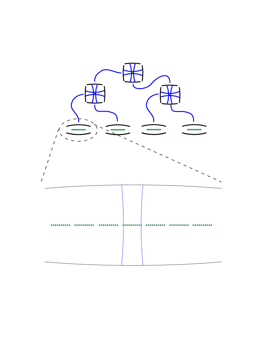
Figure 2: Hierarchical design for a quantum computer. The qubits are in groups of about 10. The physical mechanism of the computer allows gates between any pair in a group, and between the end qubits of each group and their nearest neighbours. Around 10 such groups form a block (the illustration shows 7 groups per block). Each block is coupled to the others by another physical mechanism, such as an optical method, and this allows quantum communication across long distances in the computer. To allow any one block to communicate with one of several others, switching networks may be necessary, as illustrated.

However, any such estimates involve assumptions not only about what codes and fault tolerant techniques are employed, but also about what degree of communication and of parallelism the physical hardware of the quantum computer allows. By communication we mean the ease with which one qubit can be coupled in a quantum gate with any other, not necessarily a neighbouring one. By parallelism we mean the degree to which operations can be carried out simultaneously on different sets of qubits. The case considered in [28] assumed that controlled multiple-not operations, in which a single control qubit is coupled to multiple target qubits, would be possible within each block of 127 qubits in a single time step, that operations in different blocks could be done in parallel, and that qubits in one block could be coupled to qubits in any one of several other blocks without introducing extra operations to cover communication problems. Unfortunately, it is not clear whether these assumptions are realistic.

High parallelism and ready communication tend to be mutually exclusive. At one extreme is the case of only nearest-neighbour interactions, i.e. limited communication, but any number of (logically mutually consistent) operations can be carried out in parallel. It was shown in [29] that in this case fault-tolerant methods can succeed, but no estimate of the noise threshold has yet been made. It is certainly not as high as the figures just quoted, which assumed much better communication. At the other extreme is the case of perfect communication, that is any qubit can communicate directly with any other, through a single shared degree of freedom such as a photon mode or the motion of ions in a single trap, but with no parallelism for gates involving more than one qubit. It is unlikely that this case can be stabilized sufficiently to allow large quantum computations.

Obviously the most robust physical system will be one which combines good parallelism with good communication, but the extreme case of full parallelism and direct communication between every pair of qubits is almost certainly not optimal because any process which allows such a high degree of inter-qubit coupling will have correspondingly high unwanted coupling to noisy degrees of freedom. I propose that the best construction for a quantum computer is a hierarchical one, as illustrated in figure 2. The most important role of the parallelism and communication inside the computer is to get the syndromes out as quickly as possible, so that qubits are not left accumulating noise for too long before they are corrected. The syndrome extraction operation, when carried out in a fault-tolerant manner, is itself hierarchical, because many two-bit logic gates are needed between qubits in each ancilla block, while coupling between one block and another is needed less frequently, and distant blocks need to communicate the least. The idea of the hierarchical quantum computer is that the physical hardware should reflect this logical state of affairs if an optimal robustness against noise is to be achieved.

Acknowledgements

I thank the organisers of the workshop. This work was supported by EPSRC and the European Community network QUBITS.

References

- [1] H.-K. Lo, S. Popescu, and T. Spiller, editors. Introduction to quantum computation and information. World Scientific, Singapore, 1998.
- [2] D. Bouwmeester, A. Ekert, and A. Zeilinger, editors. The physics of quantum information. Springer-Verlag, Berlin, 2000.
- [3] Michael A. Nielsen and Isaac L. Chuang. Quantum Computation and Quantum Information. Cambridge University Press, Cambridge, 2000.
- [4] P. W. Shor. Scheme for reducing decoherence in quantum computer memory. Phys. Rev. A, 52:R2493–6, 1995.
- [5] A. M. Steane. Error correcting codes in quantum theory. Phys. Rev. Lett., 77:793–797, 1996.
- [6] A. R. Calderbank and P. W. Shor. Good quantum error–correcting codes exist. Phys. Rev. A, 54:1098–1105, 1996.
- [7] A. M. Steane. Multiple particle interference and quantum error correction. Proc. Roy. Soc. Lond. A, 452:2551–2577, 1996.
- [8] E. Knill and R. Laflamme. A theory of quantum error-correcting codes. Phys. Rev. A, 55:900–911, 1997. quant-ph/9604034.
- [9] C. H. Bennett, D. P. DiVincenzo, J. A. Smolin, and W. K. Wootters. Mixed state entanglement and quantum error correction. Phys. Rev. A, 54:3825, 1996.
- [10] D. Gottesman. Class of quantum error-correcting codes saturating the quantum hamming bound. Phys. Rev. A, 54:1862–1868, 1996.
- [11] A. R. Calderbank, E. M. Rains, N. J. A. Sloane, and P. W. Shor. Quantum error correction and orthogonal geometry. Phys. Rev. Lett., 78:405–409, 1997.
- [12] A. M. Steane. Enlargement of Calderbank-Shor-Steane quantum codes. IEEE Transactions on Information Theory, 45:2492–2495, 1999.
- [13] Emanuel Knill and Raymond Laflamme. Concatenated quantum codes. quant-ph/9608012, 1996.
- [14] Dorit Aharonov and Michael Ben-Or. Fault-tolerant quantum computation with constant error rate. In Proc. 29th Ann. ACM Symp. on Theory of Computing, page 176, New York, 1998. ACM. quant-ph/9906129, quant-ph/9611025.
- [15] A. Y. Kitaev. Quantum error correction with imperfect gates. In Quantum Communication, Computing and Measurement (Proc. 3rd Int. Conf. of Quantum Communication and Measurement), pages 181–188, New York, 1997. Plenum Press.
- [16] S. J. van Enk, J. I. Cirac, and P. Zoller. Ideal quantum communication over noisy channels: a quantum optical implementation. Phys. Rev. Lett., 78:4293–4296, 1997.
- [17] S. J. van Enk, J. I. Cirac, and P. Zoller. Purifying two-bit quantum gates and joint measurements in cavity QED. Phys. Rev. Lett., 79:5178–5181, 1997.
- [18] H.-J. Briegel, W. Dür, J. I. Cirac, and P. Zoller. Quantum repeaters: The role of imperfect local operations in quantum communication. Phys. Rev. Lett., 81:5932–5935, 1998.
- [19] Andrew Steane. Quantum computing. Rep. Prog. Phys., 61:117–173, 1998.
- [20] C. H. Bennett and P. W. Shor. Quantum information theory. IEEE Transactions on Information Theory, 44:2724–2742, 1998.
- [21] A. R. Calderbank, E. M. Rains, P. W. Shor, and N. J. A. Sloane. Quantum error correction via codes over GF. IEEE Transactions on Information Theory, 44:1369–1387, 1998.
- [22] E. Knill, R. Laflamme, and L. Viola. Theory of quantum error correction for general noise. Phys. Rev. Lett., 84:2525–2528, 2000. quant-ph/9908066.
- [23] P. W. Shor. Fault-tolerant quantum computation. In Proc. 35th Annual Symposium on Fundamentals of Computer Science, pages 56–65, Los Alamitos, 1996. IEEE Press. quant-ph/9605011.
- [24] J. Preskill. Reliable quantum computers. Proc. R. Soc. Lond. A, 454:385–410, 1998.
- [25] D. Gottesman. A theory of fault-tolerant quantum computation. Physical Review A, 57:127–137, 1998. quant-ph/9702029.
- [26] D. Gottesman and I. L. Chuang. Quantum teleportation is a universal computational primitive. Nature, 402:390, 1999. quant-ph/9908010.
- [27] A. M. Steane. Active stabilisation, quantum computation, and quantum state sythesis. Phys. Rev. Lett., 78:2252–2255, 1997. quant-ph/9608026.
- [28] A. M. Steane. Efficient fault-tolerant quantum computing. Nature, 399:124–126, 1999. quant-ph/9809054.
- [29] D. Gottesman. Fault-tolerant quantum computation with local gates. Journal of Modern Optics, 47:333–45, 2000. quant-ph/9903099.