Broken promises and quantum algorithms

Abstract

In the black-box model, problems constrained by a ‘promise’ are the only ones that admit a quantum exponential speedup over the best classical algorithm in terms of query complexity. The most prominent example of this is the Deutsch-Jozsa algorithm. More recently, Wim van Dam put forward an algorithm for unstructured problems (i.e., those without a promise). We consider the Deutsch-Jozsa algorithm with a less restrictive (or ‘broken’) promise and study the transition to an unstructured problem. We compare this to the success of van Dam’s algorithm. These are both compared with a standard classical sampling algorithm. The Deutsch-Jozsa algorithm remains good as the problem initially becomes less structured, but the van Dam algorithm can be adapted so as to become superior to the Deutsch-Jozsa algorithm as the promise is weakened.

1 Introduction

It is known that for a quantum algorithm to achieve a black-box exponential speedup over a classical one, the problem in question must be constrained by a ‘promise’ (Buhrman et al., [1]). In the Black Box model of computation, where the oracle contains a set of $N$ Boolean variables $F=(f_{0},f_{1},f_{2}\ldots f_{N-1})$, about the properties of which questions can be asked (eg, ‘do all the $f_{i}$ have the value 1’, or ‘do the $f_{i}$ contain at least one 1’) through queries of the oracle, a problem with a promise is one with a restriction on the $F$s that are allowed.

The Deutsch-Jozsa problem is an example of a problem with a promise, where the question is one of deciding whether or not a given function is ‘balanced’ or ‘constant’ (each of these criteria describes a set of possible $F$ from the set of all possible $N$-bit strings and so comprises a promise as described above). We consider a relaxation of the promise on this problem (i.e., we allow extra possible $F$) and consider how this affects the efficacy of the Deutsch-Jozsa algorithm as the weakening of the promise is increased and the problem becomes less structured.

Following an introduction to the standard Deutsch-Jozsa problem (in section 2), we modify/weaken the promise on the Deutsch-Jozsa problem in section 3 and then consider the performance of the Deutsch-Jozsa algorithm on this modified problem, particularly in the limit of large numbers of input qubits and queries, providing asymptotic results. A classical algorithm based on sampling is devised to address the new problem and its success probability is considered in the same limits. In section 3.4 we introduce van Dam’s Quantum Oracle Interrogation algorithm [3] (which is designed for unstructured problems), consider how well it can be adapted to solve the modified problem and compare its performance with that of the Deutsch-Jozsa algorithm as the problem becomes less structured; this allows us to determine in which regimes one might prefer to use which algorithm.

2 The Deutsch-Jozsa Problem and Algorithm

The Deutsch-Josza problem is to recognise whether a Boolean function $f$, $\{0,1\}^{n}\stackrel{{\scriptstyle f}}{{\mapsto}}\{0,1\}$ is ‘balanced’ or ‘constant’ (that the function has one of these two properties is the promise on the problem). A constant function is one for which $f(x)$ evaluates the same, for all $x\in\{0,1\}^{n}$ (i.e., either the $f(x)$ are all $1$s or all $0$s). A balanced function is one in which $f(x)$ is equal to $0$ for exactly half of the $x$ and $1$ for the other half. This comprises a restriction on the possible contents of the oracle, $F=f_{0}f_{1}\ldots f_{N-1}$ where $N=2^{n}$ and $f_{x}=f(x)$. The Deutsch-Jozsa algorithm [4]-[6] solves this problem with one query and with no probability of error.

The input state for the Deutsch-Josza algorithm is an equal superposition of all the $|x\rangle$ such that $x\in\{0,1\}^{n}$ (constructed by acting on $|00\ldots 0\rangle$ with $H^{\otimes n}$), with an ancilla qubit in the state $\frac{1}{\sqrt{2}}(|0\rangle-|1\rangle)$. This is then acted on with the operator $U_{f}:U_{f}|x\rangle|y\mapsto|x\rangle|y\oplus f(x)\rangle$ which, given that $|y\rangle$ is the ancilla bit already described and ‘$\oplus$’ represents addition modulo $2$, has the effect of introducing a phase $(-1)^{f(x)}$ to the state $|x\rangle$. Finally an $n$-bit Hadamard is applies to the first $n$ qubits (the ancilla is discarded) and then the resulting state is measured along $|z=0\rangle$. The process, omitting the ancilla quibit, is summarised below:

$$|00\ldots 0\rangle \stackrel{{\scriptstyle H^{\otimes n}}}{{\mapsto}} \frac{1}{\sqrt{2^{n}}}\sum_{x=0}^{x=2^{n}-1}|x\rangle$$ (1)

$$\stackrel{{\scriptstyle U_{f}}}{{\mapsto}} \frac{1}{\sqrt{2^{n}}}\sum_{x=0}^{x=2^{n}-1}(-1)^{f(x)}|x\rangle$$

$$\stackrel{{\scriptstyle H^{\otimes n}}}{{\mapsto}} \frac{1}{2^{n}}\sum_{x,z=0}^{x,z=2^{n}-1}(-1)^{f(x)+x.z}|z\rangle,$$

where ‘$x.z$’ refers to the scalar product between bitstrings ($x.z=x_{1}z_{1}\oplus x_{2}z_{2}\oplus\ldots\oplus x_{n}z_{n}$). Consideration of the state $|z=0\rangle$ reveals that its amplitude is $1$ if the function is constant and $0$ if the function is balanced, so measuring along $|z=0\rangle$ will allow perfect differentiation between the cases of the function being balanced or constant. Achieving this feat classically would require examination of half of the values of $f(x)$ plus one, for a total of $2^{n-1}+1$ queries and, therefore, an exponential disadvantage as compared to the quantum algorithm.

If error is allowed, a classical algorithm needs far less queries to achieve a small error (see, eg, [2]). This algorithm progresses by looking at bits and as soon as a bit is observed which is different to previous bits, the algorithm halts and returns the result ‘balanced’, else it terminates after $k$ bits examined (i.e., $k$ queries to the algorithm) and returns ‘constant’. The only possibility of error, therefore, is when $k$ identical bits are observed (in which case the result ‘constant’ is returned) and the function is, in fact, balanced; the probability of this occurring is just the chance of selecting $k$ identical objects from a sample of two species of equal number.

$$P_{\mathrm{fail}}=2p\frac{\left(\begin{array}[]{c}N/2\\ k\end{array}\right)}{\left(\begin{array}[]{c}N\\ k\end{array}\right)}$$ (2)

where $p$ is the probability that the function is actually balanced and $N=2^{n}$. If the constant and balanced cases are equally likely and $k\ll N$,

$$P_{\mathrm{fail}}\simeq\frac{1}{2^{k}},$$ (3)

and we can see that a comparatively small number of queries $k$ can produce an accurate answer.

3 Breaking the Promise

We can imagine weakening the promise on the problem in the following way: introducing $y$ bit-flips into the $N=2^{n}$ bit string that characterises the function $f$, at random positions, would correspond to saying that the function is ‘nearly balanced’ or ‘nearly constant’, up to $y$ deviations from the promise. In this section, when we say ‘constant’ we are actually referring to ‘nearly constant’, and similarly in the case of ‘balanced’.

3.1 Deutsch-Jozsa algorithm with broken promise

The Deutsch-Jozsa (DJ) algorithm can be used unmodified on the new problem. If the function $f(x)$ is actually balanced, then in the coefficient of $|z=0\rangle$ in equation 1, we no longer see the cancellation caused by equal numbers of terms with $f(x)=1$ and $f(x)=0$ in the index of the $-1$. We now have $(\frac{N}{2}+y)$ of $\pm 1$ in the phase of $|z=0\rangle$ and $(\frac{N}{2}-y)$ of $\mp 1$. There is, therefore, a non-zero coefficient of $|z=0\rangle$, $\alpha_{0}$:

$$\alpha_{0}=\pm\frac{2y}{2^{n}},$$ (4)

which leads to an error probability $P_{\mathrm{bal}}$ of (given that error in this case is measuring $|z=0\rangle$):

$$P_{\mathrm{bal}}=y^{2}2^{2-2n}.$$ (5)

For $y$ weakenings in the promise on the actually constant $n$-bit function $f(x)$, we find that for the D-J algorithm we have:

$$\alpha_{0}=\pm\left(1-\frac{2y}{2^{n}}\right).$$ (6)

It is an error, in the case where $f(x)$ is constant, if we do do not observe $|z=0\rangle$, so our error probability in this case $P_{\mathrm{con}}$ is given by:

$$P_{\mathrm{con}}=y2^{2-n}-y^{2}2^{2-2n},$$ (7)

and we see that the error is worse if the function is actually constant than if it is balanced. Assuming that the probability that the function $f(x)$ is balanced is $p$, the error probability $P_{\mathrm{fail}}$ from one query to the quantum algorithm is:

$$P_{\mathrm{fail}} = pP_{\mathrm{bal}}+(1-p)P_{\mathrm{con}}$$ (8)

$$= py2^{2-n}-py^{2}2^{2-2n}+(1-p)y^{2}2^{2-2n}$$

$$= py2^{2-n}+(1-2p)y^{2}2^{2-2n},$$

which, where each case is equally probable ($p=\frac{1}{2}$), is given by:

$$P_{\mathrm{fail}}=y2^{1-n}$$ (9)

for a single query.

The chance of the quantum algorithm failing we assess by majority decision over $k$ queries (for direct comparison with van Dam’s algorithm and the classical case); this is the chance that $\geq\frac{k}{2}$ of the results return the wrong result (all evaluated on copies of the same function) and is given by:

$$P_{\mathrm{fail}}=\sum_{r=\frac{k}{2}}^{k}\left(\begin{array}[]{c}k\\ r\end{array}\right)\left(pP_{\mathrm{bal}}^{r}(1-P_{\mathrm{bal}})^{k-r}+(1-p)P_{\mathrm{con}}^{r}(1-P_{\mathrm{con}})^{k-r}\right).$$ (10)

We have that the mean failure probabilities for the balanced and constant strings are

$$\mu_{\mathrm{bal}} = kP_{\mathrm{bal}}=\frac{4ky^{2}}{N^{2}}$$ (11)

$$\mu_{\mathrm{con}} = kP_{\mathrm{con}}=\frac{4ky}{N}\left(1-\frac{y}{N}\right)$$ (12)

and the variances are given by:

$$\sigma^{2}_{\mathrm{bal}} = kP_{\mathrm{bal}}(1-P_{\mathrm{bal}})=\frac{4ky^{2}}{N^{2}}\left(1-\frac{4y^{2}}{N^{2}}\right)$$ (13)

$$\sigma^{2}_{\mathrm{con}} = kP_{\mathrm{con}}(1-P_{\mathrm{con}})=\frac{4ky}{N}\left(1-\frac{y}{N}\right)\left(1-\frac{4y}{N}+\frac{4y^{2}}{N^{2}}\right).$$ (14)

If we consider the limit where $y<<N$ and also that k is large enough to allow the binomial distribution to be approximated by a normal distribution, we have that

$$P_{\mathrm{fail}}\approx\frac{p}{2}\left[1-{\mathrm{erf}}\left(\frac{\frac{k}{2}-\mu_{\mathrm{bal}}}{\sigma_{\mathrm{bal}}\sqrt{2}}\right)\right]+\frac{1-p}{2}\left[1-{\mathrm{erf}}\left(\frac{\frac{k}{2}-\mu_{\mathrm{con}}}{\sigma_{\mathrm{con}}\sqrt{2}}\right)\right]$$ (15)

Since the mean value for the constant probability is smaller, the term for the ‘near-constant’ string dominates the failure probability (since we are considering probabilities at the upper tail end of the distribution). With $k$ large enough that we can use the approximation for the complementary error function, ${\mathrm{erfc}}(t)\sim e^{-x^{2}}/x\sqrt{\pi}$, and with the probabilities of actually having a balanced or constant function being equal, we have that

$$P_{\mathrm{fail}}\approx\frac{1}{4}\left[1-{\mathrm{erf}}\left(\frac{\frac{k}{2}-\mu_{\mathrm{con}}}{\sigma_{\mathrm{con}}\sqrt{2}}\right)\right]$$ (16)

so that, taking the logarithm of $P_{\mathrm{fail}}$ for ease of comparison with the other algorithms:

$$\ln P_{\mathrm{fail}} \approx -\frac{k}{32}\left(\frac{y}{N}\right)^{-1}\frac{\left[1-\frac{8y}{N}\left(1-\frac{y}{N}\right)\right]^{2}}{\left(1-\frac{y}{N}\right)\left(1-\frac{4y}{N}+\frac{4y^{2}}{N^{2}}\right)}-\frac{1}{2}\ln k+\frac{1}{2}\ln\frac{y}{N}$$ (17)

$$+ \frac{1}{2}\ln\left(1-\frac{y}{N}\right)\left(1-\frac{4y}{N}+\frac{4y^{2}}{N^{2}}\right)-\ln\left|1-\frac{8y}{N}\left(1-\frac{y}{N}\right)\right|+\frac{1}{2}\ln\frac{1}{\pi}.\ \ \ \ \ \$$

3.2 Classical algorithm with broken promise

Once we allow weakenings of the promise, the classical algorithm from section 2 becomes particularly poor; whereas previously the algorithm only failed in the case that the function was actually balanced, as the number of weakenings increases it becomes more probable that a constant function will be described as balanced and it is this probability that dominates the error probability relatively quickly. The existing algorithm is closely tied to the promise being unbroken, but a new algorithm, based on sampling, is easily designed.

This algorithm queries $k$ values of the function and then makes a decision depending on the relative numbers of bits in the sample, by counting the number of $0$s in the sample, $k_{0}$. The proportion of $0$s in the sample is used as an estimator, $\hat{p}^{cl}_{0}=\frac{k_{0}}{k}$ for the number of $0$s in the full $N$ bit string of $1$s and $0$s that describes $f$. The algorithm then infers balanced if $0.25<\hat{p}^{cl}_{0}<0.75$, or constant otherwise. This estimator is unbiased since its expected value $E(\hat{p}^{cl}_{0})=N_{0}/N$, the true proportion of zeros in the string, independent of the degree of weakening. This algorithm avoids the severe failure in the case of ‘actually constant’ from which previous classical algorithm from section 2 suffers.

This new classical algorithm fails if we have a constant (i.e., ‘weakened constant’) string and yet observe the number of $0$s, $k_{0}$, in the $k$ queries such that $\frac{k}{4}\leq k_{0}\leq\frac{3k}{4}$, or if we have ‘balanced’ and yet observe a number of $0$s, $k_{0}$, in the $k$ queries such that $k_{0}\leq\frac{k}{4}$ or $k_{0}\geq\frac{3k}{4}$ In both of these cases, the wrong inference is made.

If we describe the event ‘observing $\frac{k}{4}\leq k_{0}\leq\frac{3k}{4}$’ as $B$, the property ‘string is balanced’ as $A_{1}$ and the property ‘string is constant’ as $A_{2}$, then we can write an expression for the probability of algorithm failure, $P_{\mathrm{fail}}$, in terms of the conditional probabilities of deciding on one case given that the other is actually the case:

$$P_{\mathrm{fail}}=p\left(1-\frac{1}{2}P(B|A_{1a})-\frac{1}{2}P(B|A_{1b})\right)+(1-p)\left(\frac{1}{2}P(B|A_{2a})+\frac{1}{2}P(B|A_{2b})\right),$$ (18)

in which the subscript $a$ refers to the case when there is an excess of zeroes in the $N$ values of $f(x)$ and $b$ refers to when there is an excess of ones and, as before, $p$ is the probability that the function is actually balanced, and the classical probabilities can be well approximated by the binomial distribution in the case of ‘large’ query number, so that

$$P(B|A_{1a}) \approx \sum^{\frac{3k}{4}}_{k_{0}=\frac{k}{4}}\left(\begin{array}[]{c}k\\ k_{0}\end{array}\right)\left(\frac{1}{2}+\frac{y}{N}\right)^{k_{0}}\left(\frac{1}{2}-\frac{y}{N}\right)^{k-k_{0}}$$ (21)

$$P(B|A_{1b}) \approx \sum^{\frac{3k}{4}}_{k_{0}=\frac{k}{4}}\left(\begin{array}[]{c}k\\ k_{0}\end{array}\right)\left(\frac{1}{2}-\frac{y}{N}\right)^{k_{0}}\left(\frac{1}{2}+\frac{y}{N}\right)^{k-k_{0}}$$ (24)

$$P(B|A_{2a}) \approx \sum^{\frac{3k}{4}}_{k_{0}=\frac{k}{4}}\left(\begin{array}[]{c}k\\ k_{0}\end{array}\right)\left(1-\frac{y}{N}\right)^{k_{0}}\left(\frac{y}{N}\right)^{k-k_{0}}$$ (27)

$$P(B|A_{2b}) \approx \sum^{\frac{3k}{4}}_{k_{0}=\frac{k}{4}}\left(\begin{array}[]{c}k\\ k_{0}\end{array}\right)\left(1-\frac{y}{N}\right)^{k-k_{0}}\left(\frac{y}{N}\right)^{k_{0}}$$ (30)

In the limit of large $k$ and $y/N<1/4$, it is the ‘balanced’ string that dominates the error probability. Asymptotically we can use the central limit theorem to approximate the cumulative probability as an error function,

$$P(B|A_{1a}) \approx \frac{1}{2}{\mathrm{erf}}\left[\frac{\frac{3k}{4}-k\left(\frac{1}{2}-\frac{y}{N}\right)}{\sqrt{2k\left(\frac{1}{4}-\frac{y^{2}}{N^{2}}\right)}}\right]-\frac{1}{2}{\mathrm{erf}}\left[\frac{\frac{k}{4}-k\left(\frac{1}{2}-\frac{y}{N}\right)}{\sqrt{2k\left(\frac{1}{4}-\frac{y^{2}}{N^{2}}\right)}}\right]$$ (32)

$$P(B|A_{1b}) \approx \frac{1}{2}{\mathrm{erf}}\left[\frac{\frac{3k}{4}-k\left(\frac{1}{2}+\frac{y}{N}\right)}{\sqrt{2k\left(\frac{1}{4}-\frac{y^{2}}{N^{2}}\right)}}\right]-\frac{1}{2}{\mathrm{erf}}\left[\frac{\frac{k}{4}-k\left(\frac{1}{2}+\frac{y}{N}\right)}{\sqrt{2k\left(\frac{1}{4}-\frac{y^{2}}{N^{2}}\right)}}\right].$$ (33)

$P_{\mathrm{fail}}$ is then given by:

$$P_{\mathrm{fail}} \approx p(1-\frac{1}{2}(P(B|A_{1a}+P_{B|A_{1b}})))$$ (34)

Using the identity ${\mathrm{erf}}(-x)=-{\mathrm{erf}}(x)$ we find,

$$P(B|A_{1a})+P(B|A_{1b})\approx{\mathrm{erf}}\left[\frac{\frac{k}{4}-\frac{ky}{N}}{\sqrt{2k\left(\frac{1}{4}-\frac{y^{2}}{N^{2}}\right)}}\right]+{\mathrm{erf}}\left[\frac{\frac{k}{4}+\frac{ky}{N}}{\sqrt{2k\left(\frac{1}{4}-\frac{y^{2}}{N^{2}}\right)}}\right]$$ (35)

So that assuming $k$ is large and using the same approximation for ${\mathrm{erfc}}(x)$ as in the DJ case, we find

$$\ln P_{\mathrm{fail}} \approx -\frac{k}{8}\left[\frac{\left(1-\frac{4y}{N}\right)^{2}}{1-\frac{4y^{2}}{N^{2}}}\right]-\frac{1}{2}\ln k-\frac{1}{2}\ln\left(1-\frac{4y}{N}\right)+\ln\left(1-\frac{4y^{2}}{N^{2}}\right)+\frac{1}{2}\ln\frac{8}{\pi}\ \ \ \ \ \ \$$ (36)

3.3 Comparison of Classical and Deutsch-Jozsa algorithms

We can compare the classical and Deutsch-Jozsa algorithms, in the region where the approximations hold, through examination of equations 17 and 36. We are primarily interested in the limit where $N\gg k\gg 0$. Equating the two expressions for $\ln P_{\mathrm{fail}}$ and where $k$ is large, we have that equality in failure probability is approximately achieved by solving:

$$\frac{1}{32}\left(\frac{y}{N}\right)^{-1}\frac{\left[1-\frac{8y}{N}\left(1-\frac{y}{N}\right)\right]^{2}}{\left(1-\frac{y}{N}\right)\left(1-\frac{4y}{N}+\frac{4y^{2}}{N^{2}}\right)}-\frac{1}{8}\left[\frac{\left(1-\frac{4y}{N}\right)^{2}}{1-\frac{4y^{2}}{N^{2}}}\right]=0.$$ (37)

We see that in this regime, the solution is independent of $k$ and that the degree of weakening at which the DJ and classical algorithms yield the same failure probability tends to $y/N\approx 0.0973$. If the weakening of the promise is greater than this, the classical sampling approach works better than the DJ-based approach.

3.4 Quantum Oracle Interrogation

Since reducing the strength of the promise is akin to making the problem less structured, we compare the power of the DJ algorithm with that of an algorithm that is specifically tailored for completely unstructured problems, the Quantum Oracle Interrogation algorithm of van Dam [3, 7] (WVD). In this case, there is no promise on the problem (i.e., all possible $X$ are allowed).

As before, we use the fact that an $n$-bit function $f$ (i.e., $\{0,1\}^{n}\stackrel{{\scriptstyle f}}{{\mapsto}}\{0,1\}$ so that $N=2^{n}$) can be described by an $N$-bit string consisting of the values of $f(x)$; this is represented as a state $|F\rangle=|f_{0}f_{1}\ldots f_{N-1}\rangle$, where $f_{x}=f(x)$. An operator $A_{k}$ is introduced, the action of which depends on the Hamming weight $||x||$ of the state $|x\rangle$ (ie the number of $1$s in the binary representation of $x$):

$$A_{k}|x\rangle|b\rangle=\left\{\begin{array}[]{lc}|x\rangle|b\oplus(F.x)\rangle&\mathrm{if}\ ||x||\leq k\\ |x\rangle|b\rangle&\mathrm{if}\ ||x||>k\end{array}\right..$$ (38)

This operator requires at most $k$ queries, because the query complexity of $(F.x)$ is limited by the Hamming weight $||x||$ of $|x\rangle$, and can be carried out on states in superposition. The algorithm proceeds as follows:

• Prepare starting state $|\Psi_{k}\rangle\frac{1}{\sqrt{2}}\left(|0\rangle-|1\rangle\right)$ ($|\Psi_{k}\rangle$ depends on $k$, as is explained below)

• Act on state with $A_{k}$

• Apply $H^{\otimes N}$ to the first $N$ quibits

• Discard the ancilla qubit and measure the $N$ bits

For comparison with the previous two algorithms, we use the ‘approximate oracle interrogation’ version of WVD [3], for which the starting state $|\Psi_{k}\rangle$ is prepared as follows:

$$|\Psi_{k}\rangle=\sum_{j=0}^{k}\frac{\alpha_{j}}{\sqrt{\left(\begin{array}[]{c}N\\ j\end{array}\right)}}\sum_{\begin{subarray}{c}x\in\{0,1\}^{N}\\ ||x||=j\end{subarray}}|x\rangle.$$ (39)

Upon measurement, the observed state $|F^{\prime}\rangle$ is ‘close’ to $|F\rangle$, by which we mean that we obtain an N-bit string of which $m$ bits are correct (that is, it shares $m$ bits with $F$, so correctly represents the function $f$ for those $m$ values of $f(x)$) and the remainder incorrect, where we don’t know in which locations the correct bits are. The probability distribution for $m$ is given by

$$P(m)=1-\frac{\left(\begin{array}[]{c}N\\ m\end{array}\right)}{2^{N}}\left|\sum_{j=0}^{k}\frac{\alpha_{j}}{\sqrt{\left(\begin{array}[]{c}k\\ m\end{array}\right)}}{\mathcal{K}}_{j}(m;N)\right|^{2}$$ (40)

where ${\mathcal{K}}_{j}(m;N)$ is a Krawtchouk polynomial [8] given by

$${\mathcal{K}}_{j}(m;N)=\sum_{r=0}^{j}(-1)^{r}\left(\begin{array}[]{c}m\\ r\end{array}\right)\left(\begin{array}[]{c}N-m\\ j-r\end{array}\right).$$ (41)

We follow van Dam and use,

$$\alpha_{j}= {1\over\sqrt[4]{k}},\ \ \ k-\sqrt{k}+1\leq j\leq k$$ (42)

$$0, {\rm otherwise.}$$

For large $N$, the optimal expected number of correct bits is

$$E(m)_{opt}\approx{N\over 2}+\sqrt{k}\sqrt{N-k}.$$ (43)

and $P(m)$ becomes highly peaked around this value in the limit of large $N$ and $k$ as detailed in the appendix.

Let us consider the function $f$ which is nearly balanced or constant with $N_{0}$ zeros. We tackle the DJ problem in a similar way to the classical algorithm as discussed in section 3.2, using an estimator for the proportion of zeros in the full string ($p_{0}=N_{0}/N$). In the WVD algorithm the analogous estimator is $\hat{p}_{0}=m_{0}/N$, where $m_{0}$ is the number of zeros in the string after $k$ queries. After $k$ queries one obtains m correct bits of which $m_{0}^{*}$ are correct zeros. We assume that the correct bits are drawn at random from the full population so that the distribution of correct zeros is, in the limit of large $N$, given by

$$P(m_{0}^{*}|m)\approx\left(\begin{array}[]{c}m\\ m_{0}^{*}\end{array}\right)\left(\frac{N_{0}}{N}\right)^{m_{0}^{*}}\left(1-\frac{N_{0}}{N}\right)^{m-m_{0}^{*}}$$ (44)

with

$$E(m_{0}^{*}|m)={N_{0}\over N}m.$$ (45)

Considering each case separately in terms of the degree of weakening of the promise, $y/N$ (detailed in appendix) and assuming $k$ large

$$\mu_{1a} \approx N\left[\frac{1}{2}+\frac{2y}{N}\sqrt{\frac{k}{N}\left(1-\frac{k}{N}\right)}\right]$$ (46)

$$\mu_{1b} \approx N\left[\frac{1}{2}-\frac{2y}{N}\sqrt{\frac{k}{N}\left(1-\frac{k}{N}\right)}\right]$$ (47)

$$\mu_{2a} \approx N\left[\frac{1}{2}+\left(1-\frac{2y}{N}\right)\sqrt{\frac{k}{N}\left(1-\frac{k}{N}\right)}\right]$$ (48)

$$\mu_{2b} \approx N\left[\frac{1}{2}-\left(1-\frac{2y}{N}\right)\sqrt{\frac{k}{N}\left(1-\frac{k}{N}\right)}\right]$$ (49)

$$\sigma_{1}^{2} \approx N\left(1-\frac{4y^{2}}{N^{2}}\right)\left[\frac{1}{2}+\sqrt{\frac{k}{N}\left(1-\frac{k}{N}\right)}\right]$$ (50)

$$\sigma_{2}^{2} \approx N\left(\frac{4y}{N}\right)\left(1-\frac{y}{N}\right)\left[\frac{1}{2}+\sqrt{\frac{k}{N}\left(1-\frac{k}{N}\right)}\right]$$ (51)

We can see that $\mu$ is not an unbiased estimator for the number of zeros in the string for any of these distributions, in contrast to the previous two examples, so an inference scheme based on $N/4<m_{0}<3N/4$ implying ‘balanced’ will not be optimal where $y/N<1/4$. We must therefore shift the inference scheme to take this bias into account. The mid-points between the balanced and constant expectation values are $N(\frac{1}{2}\pm\frac{1}{2}\sqrt{\frac{k}{N}\left(1-\frac{k}{N}\right)})$. Let us therefore assume the following scheme:

$$\left|\frac{m_{0}}{N}-\frac{1}{2}\right| < \alpha\sqrt{\frac{k}{N}\left(1-\frac{k}{N}\right)}\rightarrow\mathrm{infer\ balanced}$$ (52)

$$\left|\frac{m_{0}}{N}-\frac{1}{2}\right| > \alpha\sqrt{\frac{k}{N}\left(1-\frac{k}{N}\right)}\rightarrow\mathrm{infer\ constant}.$$ (53)

In the large $N$ limit, we can assume the central limit theorem holds for these binomial distributions. The error probabilities then become:

$$P_{\mathrm{con}} \approx 1-\frac{1}{2}{\mathrm{erf}}\left[\frac{\left(1-\alpha-\frac{2y}{N}\right)\sqrt{k\left(N-k\right)}}{\sigma_{2}\sqrt{2}}\right]-\frac{1}{2}{\mathrm{erf}}\left[\frac{\left(1+\alpha-\frac{2y}{N}\right)\sqrt{k\left(N-k\right)}}{\sigma_{2}\sqrt{2}}\right]$$ (54)

$$\approx \frac{1}{2}-\frac{1}{2}{\mathrm{erf}}\left[\frac{\left(1-\alpha-\frac{2y}{N}\right)\sqrt{k\left(N-k\right)}}{\sigma_{2}\sqrt{2}}\right]$$

$$P_{\mathrm{bal}} \approx 1-\frac{1}{2}{\mathrm{erf}}\left[\frac{\left(\alpha+\frac{2y}{N}\right)\sqrt{k\left(N-k\right)}}{\sigma_{1}\sqrt{2}}\right]-\frac{1}{2}{\mathrm{erf}}\left[\frac{\left(\alpha-\frac{2y}{N}\right)\sqrt{k\left(N-k\right)}}{\sigma_{1}\sqrt{2}}\right]$$ (55)

$$\approx \frac{1}{2}-\frac{1}{2}{\mathrm{erf}}\left[\frac{\left(\alpha-\frac{2y}{N}\right)\sqrt{k\left(N-k\right)}}{\sigma_{1}\sqrt{2}}\right].$$

We now want to calculate the value of $\alpha$ to minimise $P_{\mathrm{fail}}$, so that using the fact that $\frac{d}{dx}{\mathrm{erf}}(x)=e^{-x^{2}}$, and with $k,N\gg 0$, we have that this value is given by

$$\alpha\approx 1+\frac{2y}{N}-\frac{4y^{2}}{N^{2}}-2\sqrt{\frac{y}{N}\left(1-\frac{y}{N}\right)\left(1-\frac{4y^{2}}{N^{2}}\right)}$$ (56)

so that knowledge of the quantity $y/N$ is required to optimise this inference rule, and it is this optimal value that we shall be indicating by $\alpha$ in what follows.

Finally, we have that

$$P_{\mathrm{fail}} \approx \frac{1}{2}-\frac{1}{4}{\mathrm{erf}}\left[\sqrt{k}\frac{\left(\alpha-\frac{2y}{N}\right)}{\sqrt{\left(1-\frac{4y^{2}}{N^{2}}\right)}}f(N,k)\right]-\frac{1}{4}{\mathrm{erf}}\left[\sqrt{k}\frac{\left(\alpha-\frac{2y}{N}\right)}{\sqrt{\left(\frac{4y}{N}-\frac{4y^{2}}{N^{2}}\right)}}f(N,k)\right],$$

where

$$f(N,k)^{2}=\frac{(1-\frac{k}{N})}{\left(1+2\sqrt{\frac{k}{N}(1-\frac{k}{N})}\right)}.$$ (58)

In the limit of $k>>0$ and $y/N<<1$ we find

$$P_{\mathrm{fail}} \approx \frac{1}{4}\left[1-{\mathrm{erf}}\left(\sqrt{k}\frac{\left(\alpha-\frac{2y}{N}\right)}{\sqrt{\left(1-\frac{4y^{2}}{N^{2}}\right)}}f(N,k)\right)\right]$$ (59)

$$\ln P_{\mathrm{fail}} \approx -k\frac{\left(\alpha-\frac{2y}{N}\right)^{2}}{\left(1-\frac{4y^{2}}{N^{2}}\right)}f(N,k)^{2}-\mathcal{O}\left(\ln k\right).$$ (60)

3.5 Comparison of DJ and WVD algorithms

Comparing equations 17 and 60, in the limit of $N\gg k\gg 0$, we find that the error probabilities from the DJ and WVD algorithms are approximately equal when

$$\frac{k}{32}\left(\frac{y}{N}\right)^{-1}\frac{\left[1-\frac{8y}{N}\left(1-\frac{y}{N}\right)\right]^{2}}{\left(1-\frac{y}{N}\right)\left(1-\frac{4y}{N}+\frac{4y^{2}}{N^{2}}\right)}-k\frac{\left(\alpha-\frac{2y}{N}\right)^{2}}{\left(1-\frac{4y^{2}}{N^{2}}\right)}=0$$ (61)

with $\alpha$ given by equation 56 so that the DJ and WVD algorithms in this limit share the same error probability when $y/N\approx 0.0499$. For values of $y/N$ greater than this, the WVD algorithm is superior in correctly deciding whether or not the function in question is balanced or constant, given the assumption of large $N$ and $k$. Furthermore, we note that in the region in which the given approximations hold, the classical algorithm is never better than the WVD algorithm.

4 Conclusion

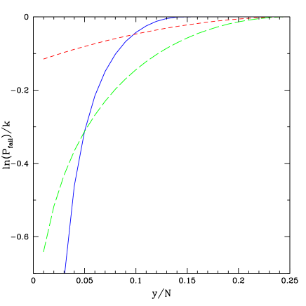
Figure 1: $\ln P_{\mathrm{fail}}/k$ against degree of weakening $y/N$, for DJ algorithm (unbroken line), WVD algorithm (long-dashed line) and classical algorithm (short-dashed line)

Figures 1, in which the relative performances of the three algorithms considered here are compared, illustrates that the problem is still structured; the DJ algorithm is successful in solving the problem but loses power as the promise becomes more broken. The WVD algorithm, which is designed for determining functions that have no promise on their nature, can be adapted to perform well even for relatively small weakenings of the promise, and becomes superior to the DJ algorithm when more than about a twentieth of the bits defining the function under examination are flipped.

We have found that the DJ algorithm is surprisingly robust when we consider breaks in the promise, with the failure probabilities driven predominantly the chance of incorrectly inferring a constant function. The speed-up in comparison to a classical sampling algorithm, in terms of queries to achieve the same result, is obviously reduced over the case of the unbroken promise, but there is still an advantage for smaller weakenings of the promise.

When compared against the quantum algorithm tailored to unstructured problems, WVD, the DJ algorithm outperforms it for low degree of weakening of the promise. The adaptation of the inference protocol for the WVD algorithm, based on the distribution of zeroes in the function string, is crucial in minimising the probability of incorrect decision, particularly for the smaller weakenings of the promise and thus the degree of the weakening of the promise needs to be known to optimise the success probability. The DJ algorithm, designed for the unbroken promise, nevertheless retains much of its advantage in the case where the promise is not greatly weakened and does not require modification according to the degree of weakening of the promise.

Given access to all three algorithms, the DJ algorithm would be preferred if the weakening of the promise was described by $y/N<.0499$ and the WVD would be preferred if the weakening was greater than this, given the assumption of large $N$, $k$ and $N\gg k$. The classical algorithm would never be preferred in this regime.

Appendix

We approach the problem by first calculating the expectation and variance of $m$ as a function of $k$ and $N$ in the large $N$ (and $k$) limit. We follow van Dam and consider a perfectly constant string of N bits all of which are zero. We then obtain the expectation and variance for the number of 1’s in the string, $t$, produced by $k$ queries and this result is then good, in fact, for the expected number of incorrect bits for any string under examination with the WVD algorithm.

Van Dam derived $E(t|N,k)$; we reproduce this result initially for completeness and then evaluate $E(t^{2}|N,k)$. The probability distribution for the number of $1$s, $t$, in the output string from the WVD algorithm is given by

$$P(t|N,k) = \sum_{i,j=0}^{k}\alpha_{i}\alpha_{j}^{*}\gamma_{ij}(N,t)$$ (62)

$$\gamma_{ij}(N,t) = \frac{1}{2^{N}}\left(\begin{array}[]{c}N\\ t\end{array}\right)\frac{{\mathcal{K}}_{i}(t;N){\mathcal{K}}_{j}(t;N)}{\sqrt{\left(\begin{array}[]{c}N\\ i\end{array}\right)\left(\begin{array}[]{c}N\\ j\end{array}\right)}}$$ (69)

We are interested in calculating the first and second moments of $t$ i.e. $E(t|N,k)$ and $E(t^{2}|N,k)$ for which we introduce the following notation:

$$\beta_{ij}^{(n)}(N,t) = \sum_{t=0}^{N}t^{n}\gamma_{ij}(N,t)$$ (70)

$$E(t^{n}|N,k) = \sum_{i,j=0}^{k}\alpha_{i}\alpha_{j}^{*}\beta_{ij}^{(n)}$$ (71)

We use the following Krawtchouk polynomial identities: the orthogonality relation of the Krawtchouk polynomials [8]

$$\sum_{t=0}^{N}\left(\begin{array}[]{c}N\\ t\end{array}\right){\mathcal{K}}_{i}(t;N){\mathcal{K}}_{j}(t;N)=2^{N}\left(\begin{array}[]{c}N\\ j\end{array}\right)\delta_{ij}$$ (76)

and the three-term recursion relation [8]

$$(N-2t){\mathcal{K}}_{j}(t;N)\equiv(j+1){\mathcal{K}}_{j+1}(t;N)+(N-j+1){\mathcal{K}}_{j-1}(t;N)$$ (77)

Multiplying 77 by $2^{-N}\left(\begin{array}[]{c}N\\ t\end{array}\right)\mathcal{K}_{i}(t;N)/\sqrt{\left(\begin{array}[]{c}N\\ i\end{array}\right)\left(\begin{array}[]{c}N\\ j\end{array}\right)}$, summing over $t$ and invoking the orthogonality relation 76 we find

$$\beta_{ij}^{(1)}=\frac{N}{2}\delta_{i,j}-\frac{1}{2}\sqrt{i(N-i+1)}\delta_{i,j+1}-\frac{1}{2}\sqrt{(i+1)(N-i)}\delta_{i,j-1}$$ (78)

so that taking WVD’s weightings $\alpha_{i}=k^{\frac{1}{4}}$ for $k-\sqrt{k}\leq j\leq k$ and 0 otherwise,

$$E(t|N,k) = \sum_{i=0}\frac{N}{2}|\alpha_{i}|^{2}-\frac{1}{2}\sqrt{(i+1)(N-i)}(\alpha_{i+1}^{*}\alpha_{i}+\alpha_{i}^{*}\alpha_{i+1})$$ (79)

$$= \frac{N}{2}-\frac{1}{\sqrt{k}}\sum_{j=k-\sqrt{k}}^{k}\sqrt{(i+1)(N-i)}$$ (80)

In the limit that $k,N>>1$ then each of the $\sqrt{k}$ terms in the sum is approximately of the order $\sim\sqrt{k(N-k)}$ and we can approximately write

$$E(t|N,k) \approx \frac{N}{2}-\sqrt{k(N-k)}+{\mathcal{O}}(\sqrt{N})$$ (81)

In order to calculate the variance we need to evaluate $E(t^{2}|N,k)$. We evaluate $\beta^{(2)}_{ij}$ by squaring the identity 77 and then, again, multiplying by $2^{-N}\left(\begin{array}[]{c}N\\ t\end{array}\right)\mathcal{K}_{i}(t;N)$, summing over $t$ and invoking the orthogonality relation 76

$$LHS \equiv N^{2}\left(\begin{array}[]{c}N\\ i\end{array}\right)\delta_{i,j}-4N\left(\begin{array}[]{c}N\\ i\end{array}\right)\left[\frac{N}{2}\delta_{i,j}-\frac{1}{2}\sqrt{i(N-i+1)}\delta_{i,j+1}\right.$$ (89)

$$\left.-\frac{1}{2}\sqrt{(i+1)(N-i)}\delta_{i,j-1}\right]+\frac{4}{2^{N}}\sum_{t=0}^{N}t^{2}\left(\begin{array}[]{c}N\\ t\end{array}\right)K_{i}(t,N)K_{j}(t,N)$$

$$RHS \equiv (i+1)(j+1)\left(\begin{array}[]{c}N\\ i+1\end{array}\right)\delta_{ij}+(i+1)(N-j+1)\left(\begin{array}[]{c}N\\ i+1\end{array}\right)\delta_{i+1,j-1}$$ (99)

$$+(N-i+1)(j+1)\left(\begin{array}[]{c}N\\ i-1\end{array}\right)\delta_{i-1,j+1}+(N-i+1)(N-j+1)\left(\begin{array}[]{c}N\\ i-1\end{array}\right)\delta_{ij}$$

It is only the diagonal terms and the off-diagonal terms differing by $|i-j|=1$ and $|i-j|=2$ that are non-zero and we find that:

$$\begin{array}[]{lcll}\beta^{(2)}_{ij}&=&\frac{1}{4}((i+1)(N-i)+i(N-i+1)+N^{2})&\mathrm{if\ }i=j\\ &=&-\frac{1}{2}N\sqrt{i(N-i+1)}&\mathrm{if\ }i=j+1\\ &=&-\frac{1}{2}N\sqrt{(i+1)(N-i)}&\mathrm{if\ }i=j-1\\ &=&\frac{1}{4}\sqrt{(N-i)(N-i-1)(i+1)(i+2)}&\mathrm{if\ }i+1=j-1\\ &=&\frac{1}{4}\sqrt{(N-i+2)(N-i+1)(i-1)i}&\mathrm{if\ }i-1=j+1\\ &=&0&\mathrm{otherwise}\end{array}$$ (101)

so, therefore, assuming WVD’s choice of weighting $\alpha_{i}$

$$E\left(t^{2}|N,k\right) = \frac{1}{4\sqrt{k}}\sum_{i=k-\sqrt{k}}^{k}\left(i+1\right)\left(N-i\right)+i\left(N-i-1)\right)+N^{2}$$ (102)

$$-\frac{1}{2}\frac{2}{\sqrt{k}}\sum_{i=k-\sqrt{k}}^{k-2}\sqrt{\left(i+1\right)\left(N-i)\right)}$$

$$+\frac{1}{4}\frac{2}{\sqrt{k}}\sum_{i=k-\sqrt{k}}^{k-2}\sqrt{\left(N-i\right)\left(N-i-1)\right)\left(i+1\right)\left(i+2\right)}$$

$$\stackrel{{\scriptstyle k,N>>1}}{{\approx}} \frac{N^{2}}{4}+k\left(N-k\right)-N\sqrt{k\left(N-k\right)}+\mathcal{O}(N)$$

and recalling that $m=N-t$, we find in the limit of $k,N>>1$

$$E(m) \approx N-E(t)=\frac{N}{2}+\sqrt{k(N-k)}$$ (103)

$$Var\left(m\right) = Var\left(t\right)=E\left(t^{2}\right)-\left[E\left(t\right)\right]^{2}$$ (104)

$$\approx \frac{N^{2}}{4}+k\left(N-k\right)-N\sqrt{k\left(N-k\right)}-\left[\frac{N}{2}-\sqrt{k(N-k)}\right]^{2}$$

$$\approx 0.$$

We can therefore assume that on exiting the quantum query algorithm we know that effectively a fixed number of bits, $m=\frac{N}{2}+\sqrt{k(N-k)}$ are correct. We assume that the algorithm knows nothing of the nature of the bits and therefore correctly or incorrectly ascertains a given bit’s value randomly so that the number of correct zeros is given by, in limit of large $N$,

$$P(m_{0}^{*}|m)=\left(\begin{array}[]{c}m\\ m_{0}^{*}\end{array}\right)\left(\frac{N_{0}}{N}\right)^{m_{0}^{*}}\left(\frac{N-N_{0}}{N}\right)^{m-m_{0}^{*}}$$ (105)

with

$$E(m_{0}^{*}) = \frac{N_{0}}{N}m=\frac{N_{0}}{N}\left(\frac{N}{2}+\sqrt{k(N-k)}\right)$$ (106)

$$Var(m_{0}^{*}) = \frac{N_{0}}{N}\left(1-\frac{N_{0}}{N}\right)\left(\frac{N}{2}+\sqrt{k(N-k)}\right)$$ (107)

so that, given $m_{0}=N-N_{0}-m+2m_{0}^{*}$ and using equations 103 and 104

$$\mu=E(m_{0}) \approx N\left[\frac{1}{2}+\left(2\frac{N_{0}}{N}-1\right)\sqrt{\frac{k}{N}\left(1-\frac{k}{N}\right)}\right]$$ (108)

$$\sigma^{2}=Var(m_{0}) \approx 4N_{0}\left(1-\frac{N_{0}}{N}\right)\left[\frac{1}{2}+\sqrt{\frac{k}{N}\left(1-\frac{k}{N}\right)}\right]$$ (109)

Considering each case separately in terms of the degree of weakening of the promise and substituting for $N_{0}$ in terms of $y,N$, we obtain equations 46-51.

References

• [1] R. Beals, H. Buhrman, R. Cleve, M. Mosca and R. de Wolf Quantum Lower Bounds by Polynomials Proceedings of FOCS ’98, 8-11 November in Palo Alto, USA, (1998) 352-361.
• [2] J. Preskill Lecture Notes on Quantum Computation, Physics 219 (Available at www.theory.caltech.edu/people/preskill/ph229/#lecture, 1997)
• [3] Wim van Dam Quantum Oracle Interrogation: Getting all the information for almost half the price. Proceedings of FOCS’98, 8-11 Novemember in Palo Alto, USA (1998) 362-369
• [4] D. Deutsch Quantum Theory, the Church-Turing Principle and the universal quantum computer Proc. R. Soc. Lond. A, 400(1985) 97-117
• [5] D.Deutsch and R. Jozsa Rapid solutions of problems by quantum parallelism Proc. R. Soc. Lond. A, 439(1992) 553-558, 1992
• [6] R.Cleve, A.Ekert, C.Machiavello and M.Mosca Quantum algorithms revisited Proc. R. Soc. Lond. A, 454(1969) 339-354, 1998
• [7] Wim van Dam, Appendix D in On Quantum Computation Theory, Ph.D. thesis, ILLC Dissertation Series 2002-04, University of Amsterdam, The Netherlands, 2002
• [8] MacWilliams, F.J. and Sloane, N.J.A.,The theory of error-correcting codes, North-Holland Publishing Company, New York, 1977, Ch. 5. §7. Theorems 16 and 19.