On the suppression of the diffusion and the quantum nature of a cavity mode. Optical bistability; forces and friction in driven cavities

Abstract

A new analytical method is presented here, offering a physical view of driven cavities where the external field cannot be neglected. We introduce a new dimensionless complex parameter, intrinsically linked to the cooperativity parameter of optical bistability, and analogous to the scaled Rabbi frequency for driven systems where the field is classical. Classes of steady states are iteratively constructed and expressions for the diffusion and friction coefficients at lowest order also derived. They have in most cases the same mathematical form as their free-space analog. The method offers a semiclassical explanation for two recent experiments of one atom trapping in a high $\mathcal{Q}$ cavity where the excited state is significantly saturated. Our results refute both claims of atom trapping by a quantized cavity mode, single or not. Finally, it is argued that the parameter newly constructed, as well as the groundwork of this method, are at least companions of the cooperativity parameter and its mother theory. In particular, we lay the stress on the apparently more fundamental role of our structure parameter.

1 Introduction

In 1994, Kimble (1994) quoted the necessity of theoretical work to be done in order to understand the dynamics of an atom in a cavity where the mode is not a prescribed quantity but rather a fully playing actor. A forefront difficulty is to draw an efficient theoretical framework that treats the strong coupling regime in open systems, externally fed, and dissipating by cavity decay $\kappa$ and/or spontaneous emission $\gamma$. The first area of cavity QED is usually devoted to coherent aspects of the coupling $g$ between the atom and the cavity mode. It is well treated within the dressed states formalism (Cohen-Tannoudji 1990), a vision that contains in block all the information about the quantized field plus the atom and where, at first, dissipation and driving are not accounted for. On the other hand, driving a cavity leads to dissipative structures. Those are well understood within the semiclassical theory of optical bistability (Lugiato and Narducci 1990). Semiclassical means here that the field is factorized from the internal state of the atom, in the operatorial sense. This corresponds in bistability theory to treat the field classically by means of Maxwell-Bloch equations. The smallness of the decay rates ($\kappa,\gamma$) allows the field to be kept inside the resonator boundaries, and hence, a long interactivity occurs before the escape of one photon or one atom. A difficulty arises as there is then a competition between the scaled Rabbi frequency of the dressed states (coherent part) and the Bonifacio-Lugiato cooperativity parameter $C=g^{2}\big{/}2\kappa\gamma$ (Bonifacio and Lugiato 1978,1975).

Recently, two major experiments reported the trapping of an atom in a cavity containing about one photon on average (Hood et al2000, Pinkse et al2000). In both papers, the trapping times of about a millisecond and the registered signals were considered to be a signature of the quantum nature of the field. Another study (Doherty et al2000) suggested by theoretical and numerical arguments that the experiment of (Pinkse et al2000) is well understood without quantization assumption of the field. One argument was to compare the diffusion coefficient and the trapping potential which they found to be close to the free space ones (Gordon and Ashkin 1980). In contrast, the experiment of (Hood et al2000) deals with a parameter regime where the diffusion is suppressed by nearly a factor of ten when compared to the free space case. (Hood et al2000, Doherty et al2000) conclude that such high suppression is a signature of the dynamics embedded in the Jaynes-Cummings ladder of dressed states, pointing out indirectly on the quantum nature of the trapping field. (Hood et al2000) support their conclusions by citing other experiments, including (Hood et al1998), that found good agreement between the full quantum calculus and the experimental data of a heterodyne signal, on the single atom level, whereas the semiclassical bistability state equation fails.

In parallel, (Pinkse et al2000) attribute the trapping mechanisms to cavity-induced cooling (Horak et al1997, Hechenblaikner et al1998). That mechanism is based on the weak-field limit and is extendable (Domokos et al2001) to higher photon number provided a low saturation is kept. Their work follows and precedes several studies concerned with the mechanical effects of light on atoms within a cavity (see e.g Doherty et al1997, Vuletić and Chu 2000). A better understanding together with an extension of the analytical calculus to higher intensities and/or saturation, on the single atom level, seems difficult as one expects, either the inclusion of multiphoton processes within the dressed states formalism, or an extension of the bistability state equation.

Having drawn the different areas to be studied, we bear in mind that the need for the full quantum calculation to fit some experimental data does not necessarily mean that one actually deals with quantum mechanics, rather, it indicates that the known semiclassical theories are insufficient. We demonstrate in this paper that both experiments of (Pinkse et al2000, Hood et al2000) are substantially explained by a semiclassical approach. A strong result is that, even if one tunes the external laser resonantly to a dressed state, neither experiment needs the ladder of dressed states to be explained. That is true for elementary steady state quantities as well as for the diffusion and friction coefficients. To that purpose, we develop a fully analytical framework that allows one to construct the needed quantities, structure and dynamics, by taking increasing orders of the coupling $g$, without any dressed states consideration. We introduce a new physical parameter, until now un-noticed, which is efficient for the treatment of driven dissipative systems, and by essence is a cooperative quantity. The method, in this paper, is limited to the explicit construction of factorized states that are an iterative version of the bistability state equation. That is possible by introducing the idea of the referred states. The referred states allow the construction of the steady states. Six steady states are derived, their common structure is given in section 2. Those are then grouped into two distinct families, the bounced states section 3, and the polarized states section 4, typically valid for increasing saturation and photon number. Our parameter is introduced in subsection 1.2 and is discussed in subsection 2.3. Section 7 draws mathematical remarks on the role of our parameter in bistability theory. Finally, we derive three expressions for the diffusion in section 5 and two expressions for the friction in section 6. Diffusion and friction are derived in such a way as to be independent of any explicit expression of the states.

1.1 The physical system

In dealing with cavity QED one usually uses the driven Jaynes-Cummings Hamiltonian for a 2 states atom represented by the lowering and rising operators ($\sigma,\sigma^{{\dagger}}$), $\sigma\!=\!|g\rangle\langle e|$, where $|g\rangle$ and $|e\rangle$ stand for the ground and excited states respectively, and a single mode with annihilation and creation operators ($a,a^{{\dagger}}$). We consider the so-called rotating wave approximation and focus only on the internal state of the atom interacting with one cavity mode. The master equation for the reduced density matrix $\rho\,$ of the system is governed by the Liouvillian $\mathcal{L}\ (\hslash=1)$:

$$\dot{\rho}=\mathcal{L}\rho,\quad\mathcal{L}\rho=-i[H,\rho]+\gamma L_{\sigma}\rho+\kappa L_{a}\rho\ ,$$ (1a)

with the dissipative parts written in the form $$\,\,\displaystyle{L_{b}\rho=2b\rho b^{\dagger}-\rho b^{\dagger}b-b^{\dagger}b\rho},\,\, \omega_{probe}$$ for any operator b, and with the Hamiltonian (in the frame rotating with the probe frequency ):

$$H=\omega_{a}\sigma^{{\dagger}}\sigma+\omega_{c}a^{{\dagger}}a+g(a^{{\dagger}}\sigma+a\sigma^{{\dagger}})+Ea^{{\dagger}}+E^{*}a\ .$$ (1b)

Here $$\omega_{a}\, \omega_{c}\, \omega_{probe} \Delta_{a},\Delta_{c} \omega_{a}\!\!\equiv\!\omega_{atom}\!-\!\omega_{probe},\,\omega_{c}\!\equiv\!\omega_{cav}\!-\!\omega_{probe} \gamma \kappa E g x g(x)\!=\!g_{0}\!\cos(2\pi x/\lambda) \lambda g_{0} g g \mathcal{F}_{dip}$$ and are the atomic and cavity frequencies respectively, detuned with respect to the probe frequency . Although these detunings are usually labelled by (), we keep our notations in order to have the formulas more compact: (). and represent respectively the atomic and cavity-mode decay rates, is the strength of the probe field that coherently drives the cavity mode, and is the coupling that we assume real and dependent on the position of the center of mass of the atom. For illustration purposes we assume a cosine dependence along the cavity axis , , with wavelength and is the maximum of . All the results presented are independent of any particular form of the coupling . Finally, the dipole force operator reads:

$$\mathcal{F}_{dip}=-(\nabla g)F_{d}\,,\quad F_{d}=a\sigma^{{\dagger}}+a^{{\dagger}}\sigma\ .$$ (1c)

1.2 Relevant dimensionless physical parameters

In order to reach a consistent understanding of the physics of the system, we look for the relevant parameters to be formed from (1a)(1b). For $E\!=\!0$, a natural description is provided by the ladder of dressed states, whose structure is basically understood by the square of the scaled Rabbi frequency $\Omega_{n}^{2}=g^{2}(n+1)/\delta^{2}\equiv C_{n}$ (Cohen-Tannoudji 1990), where $\delta=\omega_{a}-\omega_{c}$ is the detuning mismatch and $n$ the mode quantum number. $C_{n}$ is independent of the probe frequency $\omega_{probe}$ and built by atomic and mode parameters, where the latter has a discrete quantum nature. If one includes a driving, the steady state mean photon number in the cavity without the atom is given by the complex amplitude $\alpha_{0}$:

$$N_{0}\equiv\,|\alpha_{0}|^{2}\,,\quad\alpha_{0}=E/\widetilde{{\omega}}_{c}\,,\qquad(\widetilde{{\omega}}_{c}=\omega_{c}-i\kappa)\ .$$ (1b)

The parameter $\alpha_{0}$ depends upon the probe through the strength $E$ and the cavity detuning $\omega_{c}$. When the driving is sufficiently high $E\lesssim g_{0}$, a given dressed state becomes coupled to upper and lower manifolds. It becomes hard to even deduce the mean photon number $N_{0}$ from this formalism. Indeed, $\alpha_{0}$ is a continuous description of the cavity mode that tends to dismantle (dilute) the discrete dressed states by connecting them. When the atom is driven by a classical field $-\alpha$ (e.g $-\alpha_{0}$), with a strength $-g\alpha$, the relevant quantity is $g/\widetilde{{\omega}}_{a}$ ($\widetilde{{\omega}}_{a}=\omega_{a}-i\gamma$) where $|\widetilde{{\omega}}_{a}|^{2}/g^{2}$ gives the amount of (normalized) field intensity needed to saturate the atom. Symmetrically, when the atom is described by a classical dipole oscillator with polarization $\sigma\rightarrow\beta$, of strength $g\beta$, a relevant parameter for the cavity mode is $g/\widetilde{{\omega}}_{c}$, whose square modulus represents the amount of field intensity that is exchanged between the cavity and the atom (compare with $\alpha_{0}$ (1b)).

The parameters ($E/\widetilde{{\omega}}_{c},g/\widetilde{{\omega}}_{a},g/\widetilde{{\omega}}_{c}$) depend on the probe frequency $\omega_{probe}$ and, contrary to $C_{n}$, they do not describe any settled structure of the coupled-atom-mode system. A parameter accounting for that is the cooperativity parameter $C=g^{2}\big{/}2\kappa\gamma$ in bistability theory, but this quantity does not include the detunings. So we use the ratios $g/\widetilde{{\omega}}_{a}$ and $g/\widetilde{{\omega}}_{c}$ to introduce a new dimensionless complex parameter:

$$\nu\quad=\quad\displaystyle{g^{2}\over\widetilde{{\omega}}_{a}\widetilde{{\omega}}_{c}}\ .$$ (1c)

The parameter $\nu$ presents the same structure as the dressed states parameter $C_{n}$ except that it depends on the probe frequency $\omega_{probe}$ and contains no quantum signature of the cavity mode. We shall stress throughout this paper that, when the cavity mode is described classically, $\nu$ has a similar status as the (squared) scaled Rabbi frequency $C_{n}$. As $\nu$ depends on the probe frequency $\omega_{probe}$, then it is likely to be related to the driving strength $E$. We show this below. Several properties for $\nu$ should be mentioned: First it can be seen as the ratio $(g/\widetilde{{\omega}}_{c})/(\widetilde{{\omega}}_{a}/g)$, when squared it compares the number of photons (average) provided by the atom to the number of photons needed to saturate the atom. In dynamical terms, it measures the ratio between the atomic dispersive shift $g^{2}/\widetilde{{\omega}}_{a}$ and the field complex frequency $\widetilde{{\omega}}_{c}$. $\nu$ reduces to the cooperativity parameter $-2C$ when the atom and cavity are at resonance with the probe, and finally its imaginary part contains the mode-pulling formula in laser theories $\Im(\nu)\propto\kappa\omega_{a}+\gamma\omega_{c}$ (Lugiato and Narducci 1990). Finally, the deep meaning for $\nu$ is mathematically dealt with in subsection 2.3, it constitutes in this paper a central physical parameter.

1.3 A problem with the standard semiclassical factorization procedure

A description of the system that avoids the dressed states formalism could be provided by the bistability state equation, whose underlying theory is generally understood by invoking the so-called semiclassical approximation. This approximation assumes a factorization of the mean values of the product of atomic operators $A$ and mode operators $C$. It is satisfied as far as the state of the system can be factorized into a product $\rho=\rho_{m}\otimes\rho_{a}$, where ($\rho_{m},\rho_{a}$) are states for the mode (m) and the atom (a) respectively. With the notations, $\tr(CA\rho)\equiv<\!CA\!>$, $\tr(C\rho_{m})\equiv<\!C\!>$, $\tr(A\rho_{a})\equiv<\!A\!>$, that reads:

$$<\!CA\!>=<\!C\!><\!A\!>\ .$$ (1d)

The Heisenberg equations of motion for ($<\!\dot{a}\!>,$$<\!\dot{\sigma}\!>$$,<\!\dot{\sigma}_{z}\!>$), with the population difference $\displaystyle{\sigma_{z}=\sigma^{{\dagger}}\sigma\!-\!\sigma\sigma^{{\dagger}}}$ ($<\!\dot{\sigma}^{{\dagger}}\!>=<\!\dot{\sigma}\!>^{*}$ is implicit), are written:

$$<\!\dot{\sigma}\!>=-i\widetilde{{\omega}}_{a}(<\!\sigma\!>-\,\frac{g}{\widetilde{{\omega}}_{a}}<\!a\sigma_{z}\!>)$$ (1ea)

$$<\!\dot{a}\!>=-i\widetilde{{\omega}}_{c}(<\!a\!>\,+\,\alpha_{0}\,+\frac{g}{\widetilde{{\omega}}_{c}}<\!\sigma\!>)$$ (1eb)

$$<\!\dot{\sigma}_{z}\!>=-2\gamma-2\gamma<\!\sigma_{z}\!>+2ig(<\!a^{{\dagger}}\sigma\!>\!-\!<\!a\sigma^{{\dagger}}\!>)\ .$$ (1ec)

By the use of (1d), the closed system is solved at steady state; by eliminating the atomic variables ($<\!\sigma\!>,<\!\sigma^{{\dagger}}\!>,<\!\sigma_{z}\!>$), one obtains the bistability state equation for the output field $\alpha_{ob}\equiv-<\!a\!>$:

$$\alpha_{ob}\,=\,\alpha_{0}\,[\,1-\frac{\nu}{1+s_{ob}}\,]^{-1}\,,\quad s_{ob}=2\frac{g^{2}}{|\widetilde{{\omega}}_{a}|^{2}}|\alpha_{ob}|^{2}\ ,$$ (1ef)

where $s_{ob}$ stands for the corresponding atomic saturation parameter, $<\!\sigma_{z}\!>=-1/(1\!+\!s_{ob})$. Notice that, written in terms of $\nu$ (1c), the equation obtained is much clearer in form than the usual expression (Lugiato and Narducci 1990, also see section 7). That equation is cubic in the steady state output intensity $|\!\!<a>\!\!|^{2}=|\alpha_{ob}|^{2}$, thus it would possibly lead to a hysteresis cycle. The non-linear S-shape of the bistability state equation is up to now unobserved on the single atom level. (Hood et al1998) demonstrated a clear disagreement between the measured heterodyne detection and the semiclassical bistability state equation, while the data are still well explained by the exact steady state of the system (1a)(1b).

2 General formalism

2.1 Iterative factorization procedure: Definition of the referred states

Our criticism to the above procedure is based on the remark that the expectation values ($<\!a\!>,<\!\sigma\!>,$$<\!\sigma^{{\dagger}}\!>,<\!\sigma_{z}\!>$) are all considered as variables in (1ea)(1eb)(1ec). Whether they appear directly or they are issued from the factorization assumption (1d). Mainly there is no other choice than to deduce the explicit values by solving the system to obtain equation (1ef).

Our approach is still to construct factorized states, but we treat each dynamical equation (1ea)(1eb)(1ec) independently and iteratively, with assumption (1d) viewed differently for each operator product of the form $CA$, at each step. A specific example is provided to illustrate our method. A low saturation regime is assumed, the exact steady state $\rho_{s}$ corresponds to an atom almost in the ground state $|g\rangle$, $<\!\sigma_{z}\!>_{s}\approx\!-1$ (vanishing saturation parameter). Moreover, the exact mean values of product operators $CA$ can be written in the form of a product of mean values. Eventually, the low saturation regime is chosen such that one has for the bistability state equation $s_{ob}\!\gg\!1$, hence (1ef) is a bad (factorized state) approximation. Given these conditions, we approximate the exact steady state $\rho_{s}$ by $\rho_{s}\!\approx\!\rho_{m}\otimes|g\rangle\langle g|$, for the mean value $<\!a\sigma_{z}\!>$ only at this step, $<\!a\sigma_{z}\!>\approx\!-<\!a\!>$, to obtain $<\!\sigma\!>$ (1ea), that is then replaced in (1eb) to obtain $<\!a\!>=-\alpha_{0}/(1-\nu)$. We then assume that $<\!a^{{\dagger}}\sigma\!>$ factorizes according to (1d), to deduce $<\!\sigma_{z}\!>$ from (1ec). Those first steps give,

$$\alpha=\frac{\alpha_{0}}{1-\nu}\ ,\quad<\!\sigma_{z}\!>=-1+s\ ,\quad<\!\sigma\!>=\frac{g\alpha}{\widetilde{{\omega}}_{a}}\ ,$$ (1ega)

where we have defined $$\alpha\!\equiv\!-<\!a\!> s=2g^{2}/|\widetilde{{\omega}}_{a}|^{2}\times|\alpha|^{2} \alpha s\ll 1 <\!\sigma_{z}\!>\approx-1/(1+s) <\!\sigma\!> <\!\dot{\sigma}\!>=0 <\!a\sigma_{z}\!>=<\!a\!><\!\sigma_{z}\!>=\alpha/(1+s) <\!\sigma\!>,<\!\sigma_{z}\!> <\!a^{{\dagger}}\sigma\!>$$, and is the saturation parameter. The value of just deduced corresponds to the mean value of the field in the very low saturation regime (Hechenblaikner et al1998). An iteration is then started. These equations are valid for , so one can put , we then deduce by setting one more time (1ea) and use (1d) where the product is now treated as . Those procedures correctly normalize the populations, and we check that (1ec) is exactly cancelled if we use the values () just deduced and assume (1d) for . The iteration is stopped here without treating (1eb) a second time, otherwise, as shown in the next section, another state is obtained. The final equations are:

$$\alpha=\frac{\alpha_{0}}{1-\nu}\ ,\quad<\!\sigma_{z}\!>=-\frac{1}{1+s}\ ,\quad<\!\sigma\!>=\frac{g\alpha}{\widetilde{{\omega}}_{a}}\frac{1}{1+s}\ .$$ (1egb)

Those equations cannot be deduced by (1ef), where one would set $s_{ob}=0$, because we are assuming $s_{ob}\gg 1$ (an example is illustrated in the next section).

At this stage, three remarks are given. Firstly, as we treated equation (1eb) only once, the value $<\!a\!>=-\alpha$ is the same in (1ega)(1egb) and it has been deduced by using the ground state $|g\rangle$. As we assume low saturation, $|g\rangle$ is close to the final state verifying (1egb), but we distinguish it from the latter because strictly speaking one has $<\!\sigma_{z}\!>\neq-1$. The ground state $|g\rangle$ plays the role of a referred state that was used to construct the final state. The status of the referred states is strengthened below by the construction of other states. The second point is that, the atomic mean values in (1egb) correspond to optical Bloch equations where the atom is driven by a classical field of amplitude $-\alpha$, hence the properties are well known. Finally, the value of $\alpha$ determines entirely the atomic quantities, thus all those steps can be reduced to two steps: Firstly, one treats (1ea)(1eb) by invoking (1d) and uses the referred state to deduce $\alpha=-<\!a\!>$. From now on we write only the necessary equations:

$$\eqalign{<\!\dot{\sigma}\!>=-i\widetilde{{\omega}}_{a}(<\!\sigma\!>-\,\frac{g}{\widetilde{{\omega}}_{a}}<\!a\sigma_{z}\!>)\\ <\!\dot{a}\!>=-i\widetilde{{\omega}}_{c}(<\!a\!>\,+\,\alpha_{0}\,+\frac{g}{\widetilde{{\omega}}_{c}}<\!\sigma\!>)\ .}$$ (1egh)

Secondly, a Bloch equation description is assumed to deduce the atomic mean values. In the next section, an optical Bloch Liouvillian with a damped cavity mode is derived, its steady state $\rho_{\alpha}$ is a factorized state, it is known provided that one gives $\alpha$.

2.2 General form for the steady states

The method is based on a shift of the cavity mode by a position-dependent complex number $\alpha\equiv\alpha(x)$:

$$a\,\,=\,\,c-\alpha\ .$$ (1egia)

Such general shift is then used to describe equivalently the Liouvillian (1a) with the Hamiltonian,

$$\eqalign{H=\omega_{a}\sigma^{{\dagger}}\sigma\!-\!g\alpha\sigma^{{\dagger}}\!-\!g\alpha^{*}\sigma+\underbrace{g(c^{{\dagger}}\sigma\!+\!c\sigma^{{\dagger}})}\,+\,\omega_{c}c^{{\dagger}}c+(E\!-\!\widetilde{{\omega}}_{c}\alpha)c^{{\dagger}}+(E\!-\!\widetilde{{\omega}}_{c}\alpha)^{*}c\ ,}$$ (1egic)

with the dissipative terms ($$\kappa L_{c}\,,\,\gamma L_{\sigma} L_{a} \widetilde{{\omega}}_{c}=\omega_{c}-i\kappa \alpha \rho_{s} g(c^{{\dagger}}\sigma\!+\!c\sigma^{{\dagger}}) (E\!-\!\widetilde{{\omega}}_{c}\alpha)c^{{\dagger}}+(E\!-\!\widetilde{{\omega}}_{c}\alpha)^{*}c \rho_{s} \rho_{\alpha} \mathcal{L}_{\alpha}$$). Four components of the cavity mode dissipative part where already included in the Hamiltonian through the imaginary part of the complex frequency . If a given is found such that the contribution to the steady state from the coupling cancels approximately the contribution from the field driving term , then can be approximated by the factorized steady state of the Liouvillian ,

$$\eqalign{\mathcal{L}_{\alpha}\rho_{\alpha}=0,\quad\mathcal{L}_{\alpha}\rho_{\alpha}=-i[H_{\alpha},\rho_{\alpha}]+\kappa L_{c}\rho_{\alpha}+\gamma L_{\sigma}\rho_{\alpha}=0\\ H_{\alpha}\ =\ \omega_{c}c^{{\dagger}}c+\omega_{a}\sigma^{{\dagger}}\sigma-g\alpha\sigma^{{\dagger}}-g\alpha^{*}\sigma\ .}$$ (1egif)

The system (1egif) describes an atom driven by a classical field of amplitude $$-\alpha \dot{c}=-i\widetilde{{\omega}}_{c}c \rightarrow c\rightarrow-\alpha_{c}(t),\,\dot{\alpha}_{c}\!=\!-i\widetilde{{\omega}}_{c}\alpha_{c} \mathcal{L}_{\alpha} \rho_{\alpha}=Q_{\alpha}\left|0\right>\left<0\right| \left|0\right> c\left|0\right>\!=\!0 a -\!\alpha a\left|0\right>\!=\!-\alpha(x)\left|0\right> Q_{\alpha} \beta(x) \alpha(x)$$, i.e optical Bloch equations, and a cavity mode representing a damped displaced field (). The steady state of the cavity mode part of (1egif), as much as the corresponding diffusion and friction coefficients, can be described classically by the correspondance operatorcomplex number, . The operatorial description of the field is nevertheless maintained for convenience’s sake because in (1egif) the atom is quantized. The steady state of is a factorized state and written where is the vacuum of the displaced cavity mode, , it is a position dependent coherent state of the annihilation operator with the eigenvalue , . represents the steady state of the atom and is entirely defined by , which is in turn determined by . One can show that (see e.g Cohen-Tannoudji 1990):

$$Q_{\alpha}=\big{[}\,\sigma\sigma^{{\dagger}}+\beta\sigma^{{\dagger}}+\beta^{*}\sigma+|\beta|^{2}\,\big{]}\big{/}(1+s),$$ (1egig)

$$\beta=\frac{g}{\widetilde{{\omega}}_{a}}\alpha,\,\,s=2|\beta|^{2}\,,\qquad(\widetilde{{\omega}}_{a}=\omega_{a}-i\gamma)\ ,$$ (1egih)

where $$s\equiv s(x) 1/(1\!+\!s) \mathcal{O} \rho_{\alpha} \tr(\mathcal{O}\rho_{\alpha})\equiv<\!\!\mathcal{O}\!\!>_{\alpha}$$ is the atomic saturation parameter and ensures a unit trace. The expectation value of an operator in the steady state is given by the trace . Some expectation values to be used in this paper are:

$$\eqalign{<a^{{\dagger}}a>_{\alpha}=|\alpha(x)|^{2}\ ,\quad<\sigma_{z}>_{\alpha}=-\frac{1}{1+s(x)}\\ <\sigma>_{\alpha}=\frac{\beta(x)}{1+s(x)}\ ,\quad\ <F_{d}>_{\alpha}=-2g(x)\frac{\omega_{a}}{\omega_{a}^{2}\!+\!\gamma^{2}}\frac{|\alpha(x)|^{2}}{1+s(x)}\ ,}$$ (1egik)

where the force was calculated by (1c). Since a state $\rho_{\alpha}$ is entirely determined by a complex number $\alpha=-<\!a\!>_{\alpha}$ we shall refer to $\alpha$ as a state.

The approximation $\rho_{s}\!\approx\!\rho_{\alpha}$ is valid under the semiclassical approximation. It is in general satisfied if the time scale that characterizes the internal evolution of the atom is well separated from that of the cavity mode (bad or good cavity limits, large atomic or cavity detuning). In practice, we estimate the validity of our states by writing the dynamical equations ($\mathcal{L}_{\alpha}\rho_{\alpha}=0$):

$$<\dot{c}>_{\alpha}=-i\widetilde{{\omega}}_{c}(\alpha_{0}-\alpha+\frac{g}{\widetilde{{\omega}}_{c}}<\!\sigma\!>_{\alpha})\ ,\quad<\!\dot{\sigma}\!>_{\alpha}=0\ ,\quad<\!\dot{\sigma}_{z}\!>_{\alpha}=0$$ (1egija)

$$<\!\dot{a\sigma_{z}}\!>_{\alpha}=-i\widetilde{{\omega}}_{c}(<\!\sigma_{z}\!>_{\alpha}(\alpha_{0}\!-\!\alpha)\!-\!\frac{g}{\widetilde{{\omega}}_{c}}<\!\sigma\!>_{\alpha}))\ ,$$ (1egijb)

and look under which parameter regime the equation for $<\!\dot{c}\!>_{\alpha}$ (and $<\!\dot{a\sigma_{z}}\!>_{\alpha}$) are totally or partially cancelled. However, as higher order equations need to be analysed, we compare our states $\rho_{\alpha}$ with the numerical results.

The determination of the different values for $\alpha$ is grounded on a manipulation of the Hamiltonian (1egic) (and the dissipative parts). Other values are deduced by applying a similar reasoning to the Heisenberg equations of motion (1egh).

2.3 An atom-cavity-mode cooperative picture: ($\nu,E$) and the dressed states

In this subsection, we manipulate the Liouvillian $\mathcal{L}$ and show how $\nu$ (1c) appears mathematically. We then show a relationship between $\nu$ and $E$; and, finally, we relate $\nu$ to the dressed states. The whole reasoning comes with an intuitive picture, as well as indications on how states will be built in the next sections.

$\nu$ can appear by two consecutive operators shifts. The first shift corresponds to the choice $\alpha=E/\widetilde{{\omega}}_{c}\equiv\alpha_{0}$ in(1egic). The driving is entirely transferred to the atom, $-\!g\alpha_{0}\sigma^{{\dagger}}\!-\!g\alpha_{0}^{*}\sigma$, we cancel this term by a second shift, on the atomic operators,

$$\sigma\,\,=\,\,\Sigma+\beta\ ,$$ (1egijk)

with the convenient choice $\beta(x)=g\alpha_{0}/\widetilde{{\omega}}_{a}\equiv\beta_{0}$ (see (1egih)). The atomic driving is now exactly cancelled, and a new term from the coupling Hamiltonian comes out. Such mode-driving term, $\displaystyle{g\beta c^{{\dagger}}+g\beta^{*}c}$, is then written in terms of $\nu$ (1c) and $E$, to give:

$$\eqalign{H=\omega_{a}\Sigma^{{\dagger}}\Sigma+\omega_{c}c^{{\dagger}}c+g(c^{{\dagger}}\Sigma+c\Sigma^{{\dagger}})+\nu Ec^{{\dagger}}+\nu^{*}E^{*}c\ ,\quad(\kappa L_{c}\,,\,\gamma L_{\Sigma})\ .}$$ (1egijl)

In order to include the first reaction of the atom on the cavity mode, a third shift is operated, $c\rightarrow c-\nu\alpha_{0}$, to cancel the mode driving term $\nu E$ in (1egijl) (result not written). Once that done, one returns from $\Sigma$ to $\sigma$, and checks that these three local shifts are equivalent to one global shift, starting from the initial Hamiltonian (1egic), with $\alpha=\alpha_{0}(1+\nu)$. As we shall see, this value of $\alpha$ gives one simple and practical state. Another cycle will generate terms in $\nu^{2}$ in (1egijl), and so on. By those three local shifts, the strengh $E$ has been ’transported’ and ’crossed’ twice through the coupling term in (1egic) (underbraced term). Actually, the coupling term in (1b) plays the role of a pivot, it can be seen as the net in a Ping-Pong game between the atom and the cavity mode, where $E$ is the ball and $\nu$ is the dimensionless quantity that transports the ball.

An implicit relationship between $\nu$ and a finite value of $E$ is addressed by the following two statements. Firstly, for $E\neq 0$, $\nu$ has a natural role, as shown in the scheme above or in the bistability state equation (1ef). Secondly, this is not the case when $E=0$, unless for the trivial value $\nu=1$. The second statement is explained by setting $E=0$ in (1egic) and by shifting the atomic operators using (1egijk). One then equates each of the new driving terms, $(\widetilde{{\omega}}_{a}\beta-g\alpha)\sigma^{{\dagger}}$ and $(g\beta-\widetilde{{\omega}}_{c}\alpha)c^{{\dagger}}$ (and hermitian conjugates), to be zero. By that, it is easy to show that the condition $\alpha\neq\!0$ implies $\widetilde{{\omega}}_{a}\widetilde{{\omega}}_{c}\!=\!g^{2}$. But, this equality is impossible to satisfy unless one has simultaneously $\kappa\!=\!\gamma\!=\!0$ ($\Im(\nu)\!=\!0$) and $\omega_{a}\omega_{c}\!=\!g^{2}$ ($\Re(\nu)\!=\!1$). From that brief analysis, we extract two physical consequences. Firstly, by $E\!=\!0$ and $\kappa\!=\!\gamma\!=\!0$, one has the dressed Hamiltonian (1b), and, the condition $\omega_{a}\omega_{c}\!=\!g^{2}$ means that one is tuning the lowest dressed state $|-\rangle$ into resonance, in such case one has in fact $\omega_{-}-\omega_{probe}=(\omega_{a}+\omega_{c})/2-[4g^{2}+(\omega_{a}-\omega_{c})^{2}]^{1/2}/2=0$. Secondly, in (1egijl), as long as one decay rate only ($\kappa$ or $\gamma$) has a finite value, then $\nu\!\neq\!1$ and the atom (or mode) can never return the same probe strength $E$ to the mode (or atom) ($\nu E\neq E$). As $E$ and $\nu$ are somehow linked, we say that $\nu$ is also the ball, it is the ball that moves, and any exponent of $\nu$ says how many exchanges took place. We call our method the Ping-Pong. Graphically one can see the local shifts as a ping-pong exchange:

$${}^{E\,\longrightarrow}\,{}^{\alpha_{0}}\!_{\searrow}\nearrow{}^{\alpha_{0}\nu}\!_{\searrow}\nearrow{}^{\alpha_{0}\nu^{2}}\!_{\searrow}\nearrow{}^{\alpha_{0}\nu^{3}}...$$ (1egijma)

$$\quad\quad\quad\quad\!\!{}^{\beta_{0}}\quad\quad\quad\!\!\!{}^{\beta_{0}\nu}\quad\quad\quad\!\!\!{}^{\beta_{0}\nu^{2}}$$

or the global shifts with the reactions on the field only and where the atom is represented by the hooked arrow,

$$\alpha_{0}\hookrightarrow\alpha_{0}(1+\nu)\hookrightarrow\alpha_{0}(1+\nu+\nu^{2})\hookrightarrow...\ ,$$ (1egijmb)

the same last operation symmetric for the atom is of course possible by substituting $\alpha_{0}$ for $\beta_{0}$. The starting in (1egijma) is explicitly shown on the field, this would be reversed if the atom was driven first.

3 The bounced states

3.1 First bounced state

If one performs an infinite iteration in (1egijmb), a known serie in $\nu$ (complex number) leads to the first bounced state $\alpha=\alpha_{1b}$:

$$\alpha_{1b}\,=\,\frac{\alpha_{0}}{1-\nu}\ .$$ (1egijmna)

Those infinite iterations could be avoided by making directly a shift of $$\sigma E-\widetilde{{\omega}}_{c}\alpha+g\beta\,=0,\,\widetilde{{\omega}}_{a}\beta\,=\,g\alpha \widetilde{{\omega}}_{c}\widetilde{{\omega}}_{a}\!\neq\!g^{2}$$ in (1egic) and by cancelling the atom and mode driving terms. The two conditions obtained () give back (1egijmna) if .

That state is our example (1egb) in subsection 2.1, where the derivation has been opposed to the one that leads to the bistability state equation (1ef). We add some important comparison with the derivation proposed by (Hechenblaikner et al1998). Their calculations purport that, under weak driving, the Hilbert space can be restricted to the three states $\{\left|g,0,bare\right>,\left|g,1,bare\right>,\left|e,0,bare\right>\}$, where ’bare’ means the Fock states in the basis of $a^{{\dagger}}a$. Thus, in the equation for $<\!\dot{\sigma}\!>=\!0$ (1egh), the equality $<\!a\sigma_{z}\!\!>=\!-\!<\!a\!>$ is strictly satisfied, and all expectation values factorize. By $<\!\dot{a}\!>=\!0$ (1egh), and by the replacement $<\!a\!>\rightarrow\!-\alpha_{1b}$, we obtain (1egijmna). Actually, their atomic steady state quantities differ from ours (1egijmna)(1egif) owing to the presence of the saturation parameter $s_{1b}\!=\!s\!\neq\!0$ in the denominators of (1egik).

A part from that, firstly and by the operations above, the polarization $<\!\sigma\!>$ in the equation for $<\!\dot{\sigma}\!>=\!0$ (1egh) is proportional to the field amplitude, $<\!\sigma\!>\propto\alpha_{1b}$, and hence it has been replaced by the variable $\alpha_{1b}$. Consequently, by looking at the equation for $<\!\dot{a}\!>=\!0$ (1egh), the cavity mode ’sees’ itself because it is ’bounced’ by the atom. We call (1egijmna) a bounced state. Secondly, such state is known to be valid for higher photon number, provided that low saturation is ensured (Domokos et al2001). That means that a low saturation regime can be chosen, but with high photon number, $N_{0}\!>\!1$ and $|1\!-\!\nu|^{2}\!\leq\!1$, in order to have the state almost orthogonal to the subspace $\{\left|g,0,bare\right>,\left|g,1,bare\right>,\left|e,0,bare\right>\}$. Their derivation is restricted to weak driving, and hence we question back the operation $<\!a\sigma_{z}\!\!>=\!-\!<\!a\!>$, that is an exact one in this subspace. The problem is absent in our description, because, firstly, the state $\alpha_{1b}$ has its field part described by a coherent state, which is, in the bare basis, centered around the Fock state corresponding to a quantum number $n\!\approx\!|\alpha_{1b}|^{2}$; secondly, the use of the referred state $|g\rangle$ gives $<\!a\sigma_{z}\!\!>=\!-\!<\!a\!>$ without any weak driving assumption.

In figure 1, we plot the heterodyne transmission and the probability of the excited state as a function of the atomic detuning $\omega_{a}$. The parameters are chosen in order to make the bistability state equation no longer valid ($s_{ob}\!\gg\!1$), whereas our state (and the one derived below) reproduce reasonably well the exact curve. For those parameters, one has $<\!a\sigma_{z}\!\!>_{s}\neq<\!a\!>_{ob}<\!\sigma_{z}\!\!>_{ob}$ and $<\!a\!>_{ob}<\!\sigma_{z}\!\!>_{ob}\neq\!-\!<\!a\!>_{ob}$, whereas the exact steady state verifies $<\!a\sigma_{z}\!\!>_{s}\approx\!-\!<\!a\!>_{1b}$. For larger detunings, all curves meet, and the bistability state equation converges faster than (1egijmna).

Finally, we check the validity of that state. By (1egija), $<\!\dot{c}\!>_{\alpha}\!=\!\varepsilon$ with $\varepsilon=\!i\widetilde{{\omega}}_{c}\alpha_{0}\nu[1\!-\!\nu]^{-1}\!\times\!s_{1b}/(1+s_{1b})$. Thus, $\varepsilon\!\approx\!0$ for $(s_{1b}-0)\!\approx 0$ or $\alpha_{0}\ll 1$ or $|\nu|\ll 1$, and, by generalization to other Heisenberg equations, $\rho_{s}\!\approx\!\rho_{\alpha}$. Notice that (1egijb) is totally cancelled for the first bounced state, this is also true for $<\!\dot{a\sigma^{{\dagger}}}\!>_{\alpha}\!=\!0$. Finally, bear in mind the important condition $|\nu|\gg\!1$, or $|1\!-\!\nu|^{2}\gg\!1$ (for the photon number), that should ensure low photon number and low saturation regimes; $\alpha_{1b}\!\rightarrow\!0$ (drop in transmission), thus by (1egih) $\beta_{1b}\!\rightarrow\!0\Rightarrow\!s_{1b}\!\rightarrow\!0$.

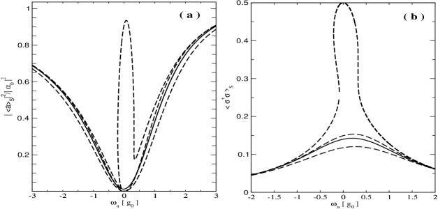
Figure 1: Comparing the bistability state equation with the exact result and our approximations. Variation with respect to the atomic detuning $\omega_{a}$. Figure(a), heterodyne transmission. From bottom to top at $\omega_{a}=g_{0}$: state(1egijmna), exact state (solid line), state(1egijmnc), bistability state equation(1ef). Figure(b), probability to be in the excited state. Same hierarchy. The parameters are $(\gamma\!=\!0.02,$$\kappa\!=\!0.6,$$\omega_{c}\!=\!0.1,$ $g_{0}\!=\!1,$$N_{0}\!=\!0.37$).

3.2 Second bounced state

This state is constructed by using the first one. As far as low saturation is achieved, (1egijmna) works for probabilities of the excited state around $<\!\sigma^{{\dagger}}\sigma\!>_{1b}\lesssim 0.1$. The increase of the driving increases the difference $s_{1b}\!-0$, which we interprete as a departure of that state (atomic part) from its own referred state, i.e the ground state $|g\rangle$. The idea is, if $s_{1b}\!-0$ is not too large, then one can iterate the procedure by viewing the first bounced state as a referred one. Therefore, we write in (1egh) $<\!a\sigma_{z}\!>=<\!a\!><\sigma_{z}\!>_{1b}$ with the population difference (1egijmna)(1egik):

$$<\sigma_{z}>_{1b}=-\frac{1}{1+s_{1b}}\ ,\qquad s_{1b}(x)=\frac{2g^{2}(x)}{|\widetilde{{\omega}}_{a}|^{2}}\frac{|\alpha_{0}|^{2}}{|1-\nu(x)|^{2}}\ ,$$ (1egijmnb)

and, as before, one deduces from (1egh) the second state $<\!a\!>\rightarrow-\alpha_{2b}$,

$$\alpha_{2b}=\frac{\alpha_{0}}{1-\nu_{1b}}\,,\quad\mbox{where}\quad\nu_{1b}(x)=\frac{\nu(x)}{1+s_{1b}(x)}\ .$$ (1egijmnc)

This state is still a bounced state, and we can see that it can be deduced by a ping-pong scheme (1egijmb) with the simple replacement $\nu\rightarrow\nu_{1b}$. The population difference of the referred state $\alpha_{1b}$ is now transported. Contrary to the first bounced state, the second one tends to $\alpha_{0}$ for increasing driving. The parameter regime where such state is valid can be understood by estimating as before (1egija). By (1egijmnc)(1egih)(1egik),

$$S_{2b}\equiv<\!\sigma\!>_{2b}\,\,=\,\,\frac{\beta_{2b}}{1+s_{2b}}\,\,=\,\,\frac{g}{\widetilde{{\omega}}_{a}}\frac{\alpha_{2b}}{1+s_{2b}}\ ,$$ (1egijmnd)

with obvious notations, $<\!\dot{c}\!>_{\alpha}\!=\!\varepsilon$ with $\varepsilon\propto\!\alpha_{0}(s_{2b}\!-\!s_{1b})$. Basically such state is valid as far as the population of the excited state is close to that of (1egijmna). In practice, it means that by keeping the atomic detuning sufficiently large, the driving can be increased to reach $<\!\sigma^{{\dagger}}\sigma\!>_{2b}\lesssim 0.2$. The intermediate photon number regime can be reached. In figure 1 this state is presented and shows better agreement than (1egijmna) because the exact population of the excited state corresponds here to values around $<\!\sigma^{{\dagger}}\sigma\!>_{s}\approx\!0.15$.

4 The polarized states

An increase of the population of the excited state leads to the appearance of the two level structure of the atom, as seen in the equation $<\sigma^{{\dagger}}\sigma>_{s}$$-<\sigma^{{\dagger}}>_{s}<\sigma>_{s}=m(s)/2$, where $m(s)\!=\!s^{2}/(1+s)^{2}$. For low saturation, $m(s)\!\sim\!s^{2}$, and hence the two level structure of the atom can be represented by the saturation parameter only. Bounced states have the property to be defined only by the saturation parameter of the referred state, and the increase of the population of the excited state transfers the steady state $\rho_{s}$ from one bounced state to another. In such regimes, the cavity mode amplitude is entirely returned by the quasi-pointlike atom ($<\!a\sigma_{z}\!>=<\!a\!><\sigma_{z}\!>_{p}$), i.e $<\!a\!>$ is a variable and $p$ is a fixed (referred) state. Else, the polarization of an atom behaves as $<\!\sigma\!>\sim\!s^{1/2}$ for low saturation and as $<\!\sigma\!>\sim\!s^{-1/2}$ for very high one. Therefore, the trick is to say that a clear appearance of the two level structure should be interpreted by treating the polarization $<\!\sigma\!>$ in the equation for $<\!\dot{a}\!>=0$ (1egh) as one object that the field ’sees’ as a whole. In this case the polarization is the referred quantity.

4.1 First polarized state

The first polarized state corresponds to the first hooked arrow in (1egijmb):

$$\alpha_{1p}\equiv\alpha_{0}(1+\nu)\ .$$ (1egijmnoa)

The reactive term $$\nu\alpha_{0} g/\widetilde{{\omega}}_{c}\times S_{ref} S_{ref} \alpha_{0} S_{ref}\!=\!g/\widetilde{{\omega}}_{a}\alpha_{0} <\!\!\sigma\!\!>_{1p} <\!\dot{c}\!>_{\alpha}\!=\!\varepsilon \varepsilon\!\propto\!-\nu\alpha_{0}[1\!-\!(1\!+\nu)/(1\!+\!s_{1p})] \varepsilon\approx 0 \nu\approx s_{1p}\,$$ can be written , where is a referred polarization of the atom because it contains no information on the actual value of the mode, but rather, it is incremented to the initial one (). The regimes where (1egijmnoa) is valid is roughly estimated by calculating , to find where . Thus for . Such a condition is a restriction but it can apply to high saturation regimes.

For the experiments of (Hood et al2000) and (Pinkse et al2000), the probe is tuned to the lowest dressed state $|-\rangle$ that is, as we said, the particular condition $\nu\approx 1$. As also $s\!\approx\!1$, (1egijmnoa) should work to give $<\!a^{{\dagger}}a\!>_{s}\approx\!4N_{0}$ at an antinode. In figure 2, we plot the mean photon number in the steady state as a function of the axial position of the atom. The agreement is satisfactory, in particular the maximum and minimum that give good agreement with the presented signals in both papers. For (Hood et al2000), the transmission reaches about $1.2-1.3$, while for (Pinkse et al2000) it goes around 4. State (1egijmnoa) is not an approximation of (1egijmna), both states meet for $\nu\!\rightarrow\!0$.

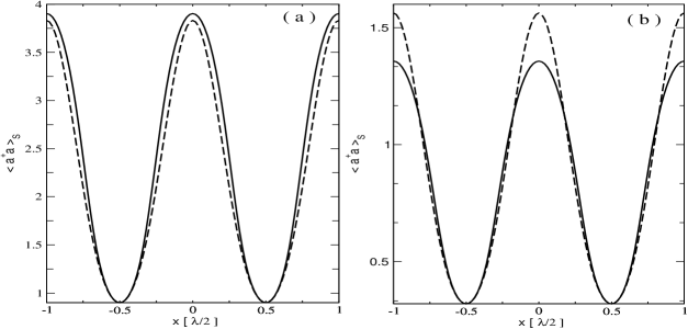
Figure 2: Mean photon number in the steady state as a function of the axial position $x\,$. Figure(a), from (Pinkse et al2000) $(\gamma\!=\!0.187,$$\kappa\!=\!0.087,$$\omega_{a}\!=\!2.8,$$\omega_{c}\!=\!0.31,$ $g_{0}\!=\!1,$$N_{0}\!=\!0.9$). Figure(b), from (Hood et al2000) $(\gamma\!=\!0.02,$$\kappa\!=\!0.13,$$\omega_{a}\!=\!1.13,$$\omega_{c}\!=\!0.7,$$g_{0}\!=\!1,$$N_{0}\!=\!0.32)$. The doted lines are $|\alpha_{1p}|^{2}\,$, the analytical formula (1egijmnoa). Solid lines are the exact numerical calculations.

4.2 Second and third polarized states

More general states can be deduced by iterating the procedures above. Bounced states are sensitive to resonances, such as $\nu\rightarrow 1$, whereas the first polarized state (1egijmnoa) is not valid for large values of $\nu$. The idea is to use both advantages.

The second polarized state is calculated by reference to the polarization (1egijmnd) of the second bounced state (1egijmnc). Consequently, this state is referred in a hierarchy to the three states (1egijmnc) (1egijmna) and the ground state. With the use of (1egijmnd), and then (1egijmnc), this gives the second polarized state ($<\!\dot{a}\!>=0$ and $<\!a\!>\rightarrow-\alpha_{2p}$):

$$\eqalign{\alpha_{2p}\equiv\alpha_{0}+\frac{g}{\widetilde{{\omega}}_{c}}S_{2b}\,\,=\,\,\alpha_{2b}(1+\nu_{q})\quad\nu_{q}=\nu_{2b}-\nu_{1b}\ ,}$$ (1egijmnoc)

where $\nu_{2b}=\nu/(1+s_{2b})$. The last equation in (1egijmnoc) shows that such state is also deduced by a ping-pong exchange, with an input field being now $\alpha_{2b}$ and a $\nu$ that transports a difference of population difference (compare with (1egijmnoa)(1egijmb)). For $s_{2b}\rightarrow s_{1b}$, the state reduces to $\alpha_{2b}$. In general, (1egijmnoc) is more flexible on the detunings, it would work for probabilities of the excited state up to $0.25\!-\!0.3$. For situations where the first bounced state (1egijmna) fails, the resulting polarized state (1egijmnoc) would smooth the results. That is the case for the experiments we discuss.

When such polarized state does not cancel resonant points, we can use the first polarized state (1egijmnoa) as the original referred state. To that end, (1egijmnoa) and (1egik) are used to form the saturation parameter $s_{1p}$ of the first polarized state; it is then regarded as a referred state to deduce a third bounced state $\alpha_{3b}$. We then calculate its polarization $S_{3b}$ (1egik), and view it as a referred state. One obtains thus the third polarized state (and the third bounced state):

$$\alpha_{3p}\equiv\alpha_{0}+\frac{g}{\widetilde{{\omega}}_{c}}S_{3b}\,\,=\,\,\alpha_{3b}(1+\nu_{q})\quad\nu_{q}=\nu_{3b}-\nu_{1p}$$ (1egijmnod)

$$\alpha_{3b}=\frac{\alpha_{0}}{1-\nu_{1p}}\,,\quad\nu_{1p}=\frac{\nu}{1+s_{1p}},\quad\big{(}s_{1p}=\frac{2g^{2}}{|\widetilde{{\omega}}_{a}|^{2}}|\alpha_{0}|^{2}|1+\nu|^{2}\big{)}\ ,$$ (1egijmnoe)

where $\nu_{3b}=\nu/(1+s_{3b})$. The third bounced state (1egijmnoe), that comes with the derivation, could work for the low saturation regimes where the other bounced states do not (typically $\nu\approx 1$). The third polarized state works well for the experiments discussed here, in particular for the heterodyne signal. However, as the atomic detuning is low, some difficulties are encountered with the regime of (Hood et al2000). Some quantum effects of the cavity mode are in fact present but we demonstrate below that they are not needed for the dynamical quantities. Eventually, those third states are like (1egijmnoa), as they are not valid for large values of $\nu$.

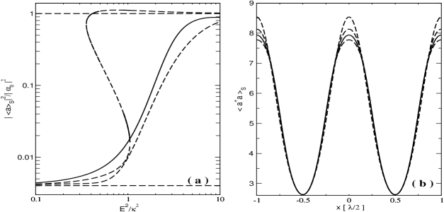
Figure 3: Figure(a), heterodyne signal as a function of the driving strength. From (Hood et al1998), $(\gamma=0.02,$$\kappa=0.33,$$\omega_{a}=\omega_{c}=0.166$,$g=g_{0}=1)$. From left to right, at ordinate 0.1: bistability state equation(1ef), exact state (solid line), state(1egijmnoc). The lowest horizontal line is the first bounced state (1egijmna). Figure(b), mean photon number as a function of the axial position. Parameters, $(\gamma=0.187,\kappa=0.094,\omega_{a}=6,\omega_{c}=1/6,g_{0}=1,N_{0}=2.63)$. From bottom to top: state(1egijmnoe), exact state (solid line), state (1egijmnoc), state(1egijmnoa). Notice the difference between the maximum and minimum for the mean photon number (intermediate regime).

In figure 3(a), we plot the heterodyne transmission as a function of the driving strength and compare it with three approximations, among which (1egijmnoc) and the bistability state equation (1ef). This plot is figure 5 of (Hood et al1998), where the experimental data fit in well with the theoretical quantum model (1b) and it constituted a part of the experimental results that supported the conclusion on the quantum nature of the field. But equation (1egijmnoc) has a classical-field interpretation. We mention, however, that other steady state quantities are not well represented for these parameters. In figure 3(b), we illustrate the intermediate photon number regime, and with $\Re(\nu)\lesssim 1$. Such parameter regime could be interesting experimentally, as it should offer a high signal to noise ratio. The reason why these polarized states work efficiently comes from the fact that we applied two different elementary procedures, the bounce and the polarization. Therefore, such states are almost stable when the parameters are varied. In counterpart, poorer results than with the other states are to be expected though.

In the next two sections are provided several expressions for the diffusion and the friction coefficients. It is believed that the arguments presented are easy to understand provided that one pays particular attention to where stationary quantities are assumed, in particular the different $\alpha$’s and $\beta$’s to be used. We repeat that the results derived below are independent of any explicit expression of the steady state quantities.

5 Diffusion at zero velocity

In the papers of (Hood et al2000, Doherty et al2000), it is suggested that the high suppression of the diffusion, when compared to the semiclassical free space case, is a relevant signature of the quantum nature of the field. As the mean photon number is around one, it was concluded that one observed single atoms bound in orbit by single photons (Hood et al2000). The semiclassical free space diffusion coefficient is calculated by assuming an equivalent standing wave of strength $<\!a\!>_{s}$, driving the atom by $g\!<\!a\!>_{s}$. The corresponding Liouvillian (Gordon and Ashkin 1980, Cohen-Tannoudji 1990) is the atomic part in (1egif), with $-\alpha\rightarrow<\!a\!>_{s}$. It leads to a diffusion about ten times (factor$\simeq 7.5$) bigger than the one obtained from the full calculus (1a)(1b). Consequently, the validity of (1egif) is questioned back, for the calculation of dynamical quantities, within the cavity QED setting. One answer is addressed by pointing at a distinction between dimensionless quantities and dynamical ones. Suppose a given Liouvillian $\mathcal{L}$ with steady state $\rho_{s}$, $\mathcal{L}\rho_{s}=0$, with eigenvectors and eigenvalues ($\rho^{k}\ ,E^{k}$), $\mathcal{L}\rho^{k}=E^{k}\rho^{k}$. If it is possible to derive a scaled Liouvillian, $\mathcal{L}_{\lambda}=\lambda\mathcal{L}$, then both Liouvillians have the same steady state and eigenvectors, but the eigenvalues differ $E^{k}_{\lambda}=\lambda E^{k}$. A dimensionless quantity, such as $<a>_{s}$, is therefore unchanged, while a dimensioned one, as the diffusion, will change according to its relation with the scaling procedure. More in accordance with our case is to suppose a Liouvillian $\mathcal{L}=\mathcal{L}_{1}+\mathcal{L}_{2}$ where ($\mathcal{L}_{1},\mathcal{L}_{2}$) have the same steady state $\rho_{s}\,$. If each sub-Liouvillian is scaled by different factors, then $\mathcal{L}_{\lambda}=\lambda_{1}\mathcal{L}_{1}+\lambda_{2}\mathcal{L}_{2}$ still has the same steady state $\rho_{s}$ as ($\mathcal{L},\mathcal{L}_{1},\mathcal{L}_{2}$) but the eigenvectors will this time differ from those of $\mathcal{L}$. Dimensionless quantities within the Hilbert space also change, except those that are evaluated at the steady state. Starting from the full Liouvillian (1b), the approximated one (1egif) offers a a good steady state structure, but fails as far as the dynamics are concerned.

5.1 Diffusion by eliminating the mode variables

A solution is found by first noting that the atomic part of (1egif) can be written by using (1egijk), ($\omega_{a}\Sigma^{{\dagger}}\Sigma\,,\gamma L_{\Sigma}$) for the Hamiltonian and the dissipative part respectively. The atomic steady state $Q_{\alpha}$ verifies independently $[\Sigma^{{\dagger}}\Sigma,Q_{\alpha}]=0$, and $L_{\Sigma}Q_{\alpha}=0$. An effective atomic Liouvillian is then derived by treating (1egh) in the operatorial form (without noise terms), by setting $\dot{a}=0$ in (1egh) and by eliminating $a$ in the equation for $\dot{\sigma}$. As the equation for $\dot{\sigma}_{z}$ is unconsidered, then $\sigma_{z}$ should be handled carefully. As long as $\sigma_{z}$ is alone, we keep it as an operator, and when it is in product with $\sigma$, it is ’frozen’ by assuming that it takes a steady state value $-1/(1+s$), given for example by some $\alpha$ and (1egik). That reads:

$$\dot{\sigma}\,=\,-i\widetilde{{\Omega}}_{a}\sigma\,-ig\alpha_{0}\sigma_{z},\quad\widetilde{{\Omega}}_{a}=\widetilde{{\omega}}_{a}(1-\frac{\nu}{1+s})\ ,$$

which could be derived by the following Liouvillian,

$$\eqalign{H_{\alpha}^{(at)}=\Omega_{a}(x)\Sigma^{{\dagger}}\Sigma,\quad\Gamma_{a}(x)L_{\Sigma},\quad\widetilde{{\Omega}}_{a}=\Omega_{a}-i\Gamma_{a}\\ \Omega_{a}(x)=\omega_{a}-\omega_{c}\frac{g^{2}(x)}{\omega_{c}^{2}+\kappa^{2}}\cdot\frac{1}{1+s(x)}\\ \Gamma_{a}(x)=\gamma+\kappa\frac{g^{2}(x)}{\omega_{c}^{2}+\kappa^{2}}\cdot\frac{1}{1+s(x)}\ ,}$$ (1egijmnopa)

where we already shifted $$\sigma \beta_{h}\equiv g\alpha_{0}/\widetilde{{\Omega}}_{a} \alpha \nu\rightarrow\nu/(1+s) \beta_{h}\approx\beta \alpha \sigma_{z} \omega_{a},\gamma$$ by an amount , that is not related to by (1egih) but directly by a supplementary infinite ping-pong exchange (1egijmb) with . As a rule, such a difference will not affect the result (because ), this supplementary bounce procedure can be seen as a way to seek fluctuations around the steady state of (1egijmnopa), which is close to the one defined by . However, if the free space steady state of (1egif) is needed, the procedure will then be stopped one step before, and hence will be frozen at some value ”before the steady state”. Actually, this procedure is performed so as to avoid non-linear equations. What is obtained is a new Liouvillian that is scaled with respect to the free space case, where the dynamical parameters () of the atom are modified by the inclusion of the reaction of the field. As we saw, the dynamics is likely to change, but with the same steady state. Finally, the dipole force is defined by:

$$\mathcal{F}_{dip}\!=-(\nabla\!g)F_{d},\quad F_{d}=-\alpha_{d}\sigma^{{\dagger}}\,-\alpha^{*}_{d}\!\sigma\ ,$$ (1egijmnopb)

with a dimensionless atomic force operator $$F_{d} \alpha_{d}\ D_{ij}$$ approximated by assuming a classical field characterized by , to be precised below. The calculation is easily deduced from the free space case. The diffusion tensor is written:

$$D_{ij}=\big{(}\nabla g\big{)}_{i}\big{(}\nabla g\big{)}_{j}\times D\ ,$$

where $$D D_{at}(\alpha_{d},s_{h})\, D_{at}(\alpha,s)\equiv D_{at}(\alpha)\, \alpha_{d}=\alpha D_{at}(\alpha,s) 12\, s_{h} 2$$ (hereafter called diffusion) is given in A.1. The result is close to the free space expression, except in a global factor slightly modified, plus a supplementary part that is in general negligible. The free-space-like term (1egijmnopqtvaa) can, in general, be approximated by . It indicates that the force (1egijmnopb) is defined by , and the saturation parameter is displaced ”one step behind”, thus returned to the steady state value. In figure 4(a) we plot for the experiment of (Hood et al2000). The free space case reaches a value around at the antinode (not shown). The suppression is well explained. By keeping the term (1egijmnopqtvy), the diffusion gets closer to the exact one and even closer if is left as it originally was (the diffusion will reach the value at the antinode).

For comparison’s sake, it is also tempting to express the force (1egijmnopb) in terms of $\alpha_{0}$, since everything is already included in the modified atomic frequency and decay rate, and the atom is driven by $-g\alpha_{0}$. In such a case, $D_{at}(\alpha_{0},s)$ is lower than the exact value. Actually, as (1egijmnopa) was used, we did not find any proper argument to legitimate one value of $\alpha_{d}$ rather than another in the expression of the force (1egijmnopb). That is seen in figure 4(a) where different values of $\alpha_{d}=(\alpha,\alpha_{0}$) approach the exact result differently. For these experiments, the dominating term in $D_{at}(\alpha_{d},s_{h})$ is the known free space diverging term in $s_{h}$: $\Gamma_{a}^{-1}|\alpha_{d}|^{2}s_{h}^{3}[1+s_{h}^{3}]^{-1}$. Here, formally, it does not diverge but reaches a constant value $\Gamma_{a}^{-1}|\alpha_{d}|^{2}$ (unless for $\alpha_{d}=\alpha$). The origin of that divergence has been interpreted (Gordon and Ashkin 1980) in terms of the dressed state approach in free space. However, the reason for the suppression with regard to the experiment of (Hood et al2000) is actually the value of $\Gamma_{a}\approx 10\gamma$ at the antinode, thus $D_{at}\approx D_{free}/10\ll D_{free}$.

5.2 Diffusion by eliminating the atomic variables

There is also a possibility to include all quantities in the field variable, by setting $\dot{\sigma}=0$ in (1egh) and inserting it in the equation for $\dot{a}$. Similar arguments to the previous case lead to:

$$\eqalign{H_{\alpha}^{(field)}=\Omega_{c}(x)c^{{\dagger}}c\,\,,\quad K_{c}(x)L_{c}\,,\ a=c-\alpha\\ \Omega_{c}(x)=\omega_{c}-\omega_{a}\frac{g^{2}(x)}{\omega_{a}^{2}+\gamma^{2}}\cdot\frac{1}{1+s(x)}\\ K_{c}(x)=\kappa+\gamma\frac{g^{2}(x)}{\omega_{a}^{2}+\gamma^{2}}\cdot\frac{1}{1+s(x)}\ ,}$$ (1egijmnopc)

where a simplification relating $\alpha$ to $s$ and $\beta$ has already been made. The latter defines then the dipole force $F_{d}=\beta a^{{\dagger}}+\beta^{*}a$. This case is trivial (we scale out the gradients):

$$D_{field}=|\beta|^{2}\frac{K_{c}}{\Omega_{c}^{2}+K_{c}^{2}}\ .$$ (1egijmnopd)

We plot in figure 4 $D\!=\!D_{field}\!+\!D_{at}(\alpha_{0},s)$ for both experiments, in figure 4(b) we also show $D\!=\!D_{field}\!+\!D_{at}(\alpha,s)$. State (1egijmnoa) can also be used, the exact result will be approached differently.

It should be clearly reminded that, in every case, Bloch equation-like and a damped displaced cavity mode are the background assumption. A picture is provided by imagining a swimmer swimming in a small pool, who consequently generates waves which get reflected by the finite size of the pool; that then changes the structure of the surface of the water to finally make the swim more difficult to the swimmer by pushing him according to the way he swims. In the end, the swimmer dissipates energy ($\Gamma_{a}\gg\gamma$) in trying to move and gets tired. In the free space limit $\kappa\rightarrow\infty$ , one has ($\Omega_{a},\Gamma_{a})\rightarrow(\omega_{a},\gamma$) and $K_{c}\sim\kappa$, and hence $D_{at}\rightarrow D_{free}$ and $D_{field}\rightarrow 0$.

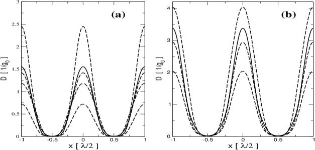
Figure 4: Diffusion coefficient $D$ as a function of the axial position. Figure(a), parameters from (Hood et al2000). Figure(b), parameters from (Pinkse et al2000). Same parameters as figure 2. From bottom to top: figure(a), $D_{at}(\alpha_{0},s)$, $D_{cav}$(1egijmnope), $D_{field}\!+\!D_{at}(\alpha_{0},s)$, exact (solid line), $D_{at}(\alpha,s)$. Figure(b), $D_{field}\!+\!D_{at}(\alpha_{0},s)$, $D_{field}\!+\!D_{at}(\alpha,s)$, exact (solid line), $D_{cav}$(1egijmnope). $\alpha$ is given by (1egijmnoc).

5.3 Diffusion by considering the atom-mode coupled system

Those previous expressions for the diffusion supposed the field or the atom as prescribed quantities. Other results are given where both objects are regarded as ”active”. This is done by solving (1egh) approximately, the procedure is analogous to (Hechenblaikner et al1998). As the population difference $\sigma_{z}$ is frozen, we consider two cases that could be grouped into one in future works. The result for the diffusion can be written $D=D_{cav}$:
with the ”high saturation” case,

$$D_{cav}=\frac{4\omega_{a}}{\omega_{a}^{2}\!+\!\gamma^{2}\!}\cdot|\alpha|^{2}\cdot\frac{|\,\alpha\,|^{2}}{|\alpha_{0}|^{2}}\frac{\Im(\nu)}{(1+s)}\ ,$$ (1egijmnope)

or the ”low saturation” case,

$$D_{cav}=\frac{4\omega_{a}}{\omega_{a}^{2}\!+\!\gamma^{2}\!}\cdot\frac{|\alpha|^{2}}{(1+s)}\cdot\frac{|\,\alpha\,|^{2}}{|\alpha_{0}|^{2}}\frac{\Im(\nu)}{(1+s)}\ .$$ (1egijmnopf)

The difference is essentialy a factor $1/(1+s)$, whose origin is related to the difference between $<\!\sigma^{{\dagger}}\sigma\!>$ and $<\!\sigma^{{\dagger}}\!><\!\sigma\!>$. An additive term $\gamma/|\widetilde{{\omega}}_{a}|^{2}\times|\alpha|^{2}/(1+s)$ has been dropped, it is a part of the free space expression and can be neglected within our approximations. If one sets $s=0$, and explicits $\alpha$ by the first bounced state expression (1egijmna), then one recovers the expression derived by (Hechenblaikner et al1998). The authors interpreted such term as cavity-induced, we explicit here its cooperative origin, indeed it is proportional to the imaginary part of $\nu$. For $\kappa\rightarrow\infty$, $\Im(\nu)\rightarrow 0$ and $D_{cav}$ cancels. Equation (1egijmnope) is plotted in figure 4. Eventually, the diffusion due to spontaneous emission is proportional to the probability of being in the excited state, thus it is given by (1egik).

6 Friction at first order in velocity

The friction coefficient is derived from the same Liouvillians (1egijmnopa)(1egijmnopc) as those for the diffusion, but we use another definition for the force. Since the friction coefficient is related to a velocity development, it is suitable to define here the force by minus the gradient of the Hamiltonians (1egijmnopa)(1egijmnopc). That force being given, we develop the expression to first order and relate its quantities to the spatial derivatives of steady state mean values. The method is a standard procedure, similar to (Gordon and Ashkin 1980, Hechenblaikner et al1998). To perform the calculus, one suggestion is first to return from the variables ($\Sigma,c$) to ($\sigma,a$) in (1egijmnopa) and (1egijmnopc), and then derive. The velocity $\mathbf{v}$ dependent force $\digamma_{v}$ is given by the coefficient $G$ (hereafter called friction):

$$\digamma_{v}=-(\mathbf{v}\cdot\nabla g)\nabla g\,G\ .$$ (1egijmnopqa)

6.1 Friction by eliminating the atomic variables

The easiest case is the cavity-mode Liouvillian (1egijmnopc), which leads to a force proportional to $a^{{\dagger}}a$. By direct derivation, one obtains an important expression:

$$\eqalign{G_{field}=4|\alpha|^{2}\frac{\xi_{c}}{\Omega_{c}^{2}+K_{c}^{2}}\Big{(}\ \frac{K_{c}\Omega_{c}}{\Omega_{c}^{2}\!+\!K_{c}^{2}}\,\xi_{c}+\frac{1}{2}\frac{\Omega_{c}^{2}\!-\!K_{c}^{2}}{\Omega_{c}^{2}\!+\!K_{c}^{2}}\,\zeta_{c}\ \Big{)}\\ \xi_{c}=2g\frac{\omega_{a}}{\omega_{a}^{2}+\gamma^{2}}\frac{1}{1+s}F(s,\nu)\ ,\quad\zeta_{c}=2g\frac{\gamma}{\omega_{a}^{2}+\gamma^{2}}\frac{1}{1+s}F(s,\nu)\ ,}$$ (1egijmnopqb)

where $s=2g^{2}|\alpha|^{2}/|\widetilde{{\omega}}_{a}|^{2}\,$ and ($\xi_{c}(x),\zeta_{c}(x)\,,F(s,\nu)$) are discussed below. For our regimes, it can generally be assumed $\zeta_{c}\!=\!0$. For ($s\!=\!0,F(s,\nu)\!=\!1$), $G_{field}$ reduces to the friction obtained by (Hechenblaikner et al1998) in the good cavity limit.

6.2 Friction by eliminating the field variables

In the other limit (1egijmnopa), the friction obtained is easily interpreted as long as a free space term $G_{free}$ is clearly recognized:

$$\eqalign{G_{at}=\ G_{free}\ +\,\xi_{a}G_{1}+\xi_{a}^{2}G_{2}+\zeta_{a}(G_{1\zeta}\!+\!\xi_{a}G_{2\zeta})\\ \xi_{a}=2g\frac{\omega_{c}}{\omega_{c}^{2}+\kappa^{2}}\frac{1}{1+s}F(s,\nu)\ ,\quad\zeta_{a}=2g\frac{\kappa}{\omega_{c}^{2}+\kappa^{2}}\frac{1}{1+s}F(s,\nu)\ ,}$$ (1egijmnopqc)

where ($G_{free},\,G_{1},\,G_{2},\,G_{1\zeta},\,G_{2\zeta}$) are functions of $(s_{h}=2|\beta_{h}|^{2},\Gamma_{a},\Omega_{a},g$) and given in A.2. Similarly to $G_{field}$, one can in general assume $\zeta_{a}\!=\!0$ for $G_{at}$. For ($\xi_{a}\!=\!0,\zeta_{a}\!=\!0$), the free space term is recovered, but it is defined by the modified frequency $\Omega_{a}$ and decay rate $\Gamma_{a}$. For ($\alpha_{0}\rightarrow 0,s_{h}\rightarrow 0,s=0,F(s,\nu)\!=\!1$), $G_{at}/N_{0}$ (1egijmnopqtvac) gives back the expression derived by (Hechenblaikner et al1998) in the bad cavity limit.

In order totally to relate the friction coefficients (1egijmnopqc)(1egijmnopqb) to steady state quantities, one still has to specify the function $F(s,\nu)$.

6.3 Expressions for the function $F(s,\nu)$

The dimensionless parameters $\xi_{a}\!\equiv\!-\partial_{g}\Omega_{a}\,$, $\xi_{c}\!\equiv\!-\partial_{g}\Omega_{c}$ (and $\zeta_{a},\zeta_{c}$) measure the sensitivity of the atom and cavity frequencies to the variations of the coupling. Some are oftentimes interpreted as trapping potentials $U(x)$ acting on the atom, $\ \xi_{c}\equiv-\partial_{g}U(x)$. In the low saturation limit, $\xi_{c}$ reduces to $2g\,\omega_{a}/(\omega_{a}^{2}+\gamma^{2})$, and can be understood by analogy with a massive pointlike damped dipole oscillator (Hechenblaikner et al1998). The inclusion of the saturation parameter, through the real function $F(s,\nu)/(1\!+\!s)$, shows the departure from which the two level structure appears. The function,

$$F(s,\nu)=1-\frac{s}{1+s}\Re\big{(}g\partial_{g}\beta/\beta\big{)}\ ,$$ (1egijmnopqr)

reduces to $1$ at zero saturation, and is related to the derivative of $\beta$. If the steady state is provided by the ping-pong schemes, then $F(s,\nu)$ contains the variation of the referred states. However, in general, there is a possibility to provide several tractable and efficient expressions for $F(s,\nu)$. An approximation is given which is part of a generalized ping-pong scheme to be dealt with elsewhere. One starts from a general bounced state expression, $\alpha=\alpha_{0}/(1-\nu_{p})$, and a polarized state $\alpha=\alpha_{0}(1+\nu_{p})$, with $\nu_{p}=\nu/(1+s_{p})$, and where $s_{p}(x)$ is the saturation parameter relative to a referred state ”p”. The derivatives $(g\partial_{g}\beta)/\beta$ become:

$$g\partial_{g}\beta/\beta\Big{|}_{bounce}=1+\frac{2\nu_{p}}{1\!-\!\nu_{p}}F(s_{p},\nu)\ ,\quad g\partial_{g}\beta/\beta\Big{|}_{pol.}=1+\frac{2\nu_{p}}{1\!+\!\nu_{p}}F(s_{p},\nu)\ ,$$ (1egijmnopqs)

and hence $F(s,\nu)$ (1egijmnopqr) is related to the function $F(s_{p},\nu)$ (1egijmnopqs) relative to the referred state ”p”. The next step is to understand what kind of approximations are most efficient; different possibilities are given:

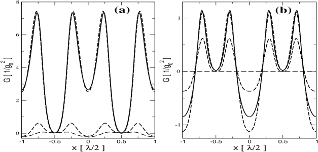
Figure 5: Friction coefficient $G$ as a function of the axial position. Figure(a), (Pinkse et al2000). From bottom to top: $G_{free}(s)$, $G_{at}(s)$, $G_{field}$, exact $G$ (solid line). We used state (1egijmnoc) and the $\nu$ dependent version (1egijmnopqtb) for the function $F(s,\nu)$. Figure(b), (Hood et al2000). From bottom to top: $G_{field}\!+\!G_{at}(s)$, exact $G$ (solid line), term $\xi_{a}G_{1}\!+\!\xi_{a}^{2}G_{2}\!+\!\zeta_{a}$$(G_{1\zeta}\!+\!\xi_{a}G_{2\zeta})$. We used state (1egijmnoc) and $F(s,\nu)$ is given by (1egijmnopqta). Notice, in figure(b), the positive contribution of the translational friction term.

$$g\partial_{g}\beta/\beta\simeq 1$$ (1egijmnopqta)

$$g\partial_{g}\beta/\beta\simeq 1+\frac{\nu}{1+s}\rightarrow 1+\frac{1}{1+s}$$ (1egijmnopqtb)

$$g\partial_{g}\beta/\beta\simeq 1+\frac{2\nu_{\alpha}}{1\!-\!\nu_{\alpha}}\rightarrow 1-\frac{2}{1+s}$$ (1egijmnopqtc)

$$g\partial_{g}\beta/\beta\simeq 1+\frac{2\nu_{\alpha}}{1\!-\!\nu_{\alpha}}F(s,\nu)\ ,$$ (1egijmnopqtd)

where $\nu_{\alpha}=\nu/(1+s)$. The referred state p has been eliminated. The first case (1egijmnopqta) assumes a variation proportional to that of a pure standing wave. The atom could be affected by the reaction of the field but, when it moves, it sees a constant strength ($\beta\simeq g\times constant$). Such approximation is generally valid for small values of $\nu$ or at high saturation (check with (1egijmnopqs)), as for (Hood et al2000). In that case, (1egijmnopqta) gives $F(s,\nu)=1/(1+s)$. The two approximations in (1egijmnopqtb) are obtained with the polarized state expression, it is assumed that the saturation parameter $s_{p}\approx s$ varies with $\nu$ as $s\!+\!\nu\lesssim 1$, and $F(s_{p},\nu)=1/(1+s)$ (pure standing wave). Such approximation is more valid at intermediate saturation $\nu\approx s\lesssim 1$. The arrow in equation (1egijmnopqtb) means that, at this step, $\nu=1$ can be assumed. Indeed, the functions ($\xi_{a},\zeta_{a},\xi_{c},\zeta_{c}$) cancel for $g=0$ and hence the relevant points are around the maximum of the coupling. In such a case, (1egijmnopqr) simplifies to give $F(s,\nu)=1/(1+s)^{2}$, and the difference of the exponent ($1+s$) with the function $F(s,\nu)$ derived from (1egijmnopqta) shows again the limit between high and low saturation. The third case (1egijmnopqtc) is aimed to work efficiently for large values of $\nu$, it is derived from the general bounced state expression. By the right arrow, we simplify the expression by taking the limit $\nu_{p}\rightarrow\infty$, and a supplementary ratio $1/(1+s)$ has been added from $F(s_{p},\nu)$. The two arrowed limits just discussed have an interest (a part simplification) because they are smoothed versions of the expressions from which they derive, that might contain some undesired resonance. Finally, (1egijmnopqtd) represents the case close to the optical bistability way-of-thinking, the value of $\beta$ is returned, thus by (1egijmnopqr), $F(s,\nu)$ can be deduced (not written). Once these procedures made, the functions $F(s,\nu)$ now depend on the saturation parameter of the steady state only, therefore one can simply forget the origin of the states that lead to (1egijmnopqs). As final simplifications, for the coefficients ($G_{free},G_{1},G_{2},G_{1\zeta},G_{2\zeta}$) (1egijmnopqtvac), one can as usual operate $s_{h}\simeq s\,$ (as for the diffusion), thus all the friction coefficients are now completely determined by providing $\alpha$.

For the experiment of (Hood et al2000), the translated terms of $G_{at}$ (1egijmnopqc) have an effect and tend to render the friction positive. This is shown in figure 5 where we also plot the friction for the experiment of (Pinkse et al2000). The friction $G_{field}$ (1egijmnopqb) is an excellent approximation for that experiment. It shows that the quantum nature of the mode is again not needed, thus responding to the questioning of (Doherty et al2000). A basic result for this paper is plotted in figure 6, it shows a situation of high positive friction and a diffusion similar to (Pinkse et al2000). The temperature is about twice as low. Also notice that, for figure 6(a), it is $G_{field}$ that works despite the fact that $\gamma<\kappa$. This is a reminder that the bad/good cavity limits are only rough limits, in figure 6(a) the opposite situation occurs. That is caused by the other physical parameters, like the coupling $g$, which are greater than $\kappa$. Actually, this exact reversion can be explained by extending the notion of bad/good cavity limits: ($\Gamma_{a},K_{c}$) are the relevant decay rates to determine which limit to use. In figure 6(a), we have in fact $\Gamma_{a}>K_{c}$, thus the hierarchy is reversed ($\gamma<\kappa$). Eventually, we present in figure 7 a cavity resonant case, with a high photon number $N_{0}\!=\!11$, high friction, and a diffusion as low as (Hood et al2000). In that case, the atom is trapped almost exactly half way between the node and the antinode, thus it experiences a non zero friction and diffusion ($\nabla g\neq 0$). Such parameters should be very efficient for trapping, with a very clear drop at the output transmission.

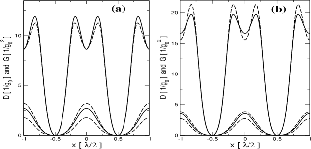
Figure 6: Diffusion and friction coefficients as a function of the axial position. Figure(a), $(\gamma=0.0236,\,\kappa\!=\!0.13,\,\omega_{a}\!=\!6,\,\omega_{c}\!=\!1/6,\,g_{0}\!=\!1,\,N_{0}\!=\!2.16)$. From bottom to top at $x=0$: $D_{field}+D_{at}(s)$, exact $D$ (solid line), $D_{cav}(\ref{Dcavunsat})$, exact $G$ (solid line), $G_{field}$. For $F(s,\nu)$, we used the $\nu$ dependent form of (1egijmnopqtc). Figure(b), same parameters as figure 3(b). From bottom to top at $x=0$: $D_{field}+D_{at}(s)$, exact $D$ (solid line), $D_{cav}$(1egijmnopf), $G_{field}$, exact $G$ (solid line). We used the $\nu$ dependent form of (1egijmnopqtb). For both figures, we used state (1egijmnoa).

7 Remarks on optical bistability theory

Our goal was first oriented towards cavity QED trapping mechanisms. It was only when $\nu$ (1c) was labelled and attributed some importance, through the first ping-pong schemes (1egijma)(1egijmb), that its interpretation became needed. Its link to the cooperative parameter $C=g^{2}\big{/}2\kappa\gamma$ (Bonifacio and Lugiato 1978) is obvious and it is standard belief that $\nu$ is a natural generalization of $C$. What is uncommon, however, is that $\nu$ is never used in the optical bistablity theory (Lugiato and Narducci 1990, Abraham and Smith 1982), as far as we are concerned. We make essentially two remarks, showing that, maybe, one could rethink optical bistability with $\nu$ and $C$ in hand. There is a standard mean-field optical bistability state equation, which is commonly written in the form (Lugiato and Narducci 1990):

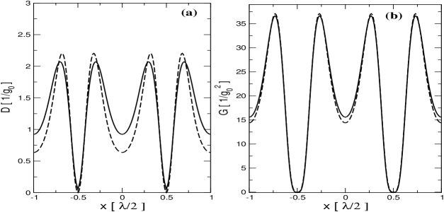
Figure 7: Diffusion and friction coefficients as a function of the axial position. Cavity resonant case. $(\gamma=0.18,\,\kappa\!=\!0.09,\,\omega_{a}\!=\!-5,\,\omega_{c}\!=\!0,\,g_{0}\!=\!1,\,N_{0}\!=\!11)$. From bottom to top at $x=0$: Figure(a), $D_{cav}$(1egijmnopf), exact $D$ (solid line). Figure(b), $G_{field}$, exact $G$ (solid line). For $F(s,\nu)$, we used the $\nu$ dependent form of (1egijmnopqtc), with state (1egijmnc). The atom should be trapped at points $x_{M}$ such that $g^{2}(x_{M})=-\omega_{a}\kappa$, with a temperature $D/G\approx 2/35g_{0}\simeq\kappa$.

$$x=y\{1+i\theta+2C(1-i\delta)/(1+\delta^{2}+|x|^{2})\}^{-1}\ ,$$ (1egijmnopqtu)

where $x,y\,$ are the scaled output and input field amplitudes respectively. That equation depends on the scaled detunings $\theta=\omega_{c}/\kappa,\delta=\omega_{a}/\gamma$ and the cooperative parameter $C$. Therefore, the space of parameters in which one works is the $(C,\delta,\theta,y)$ space; however, as one parameter is usually a variable, like for example the input amplitude $y$, bistability conditions are drawn in the cubic space $(C,\delta,\theta)$. We showed that the state equation above is actually the bounced state (1ef), scaled differently with the schematical correspondences $y\rightarrow\alpha_{0},\,x\rightarrow\alpha_{ob}$, and with a saturation parameter related to $|x|^{2}$. The referred state is here the state itself. Consequently, the space is now reduced to $(\nu,\alpha_{0})$ or ($\nu$) alone if $\alpha_{0}$ is a variable. What was to be expected does happen; we show two typical inequalities that are conditional to optical bistability (Agrawal and Carmichael 1979, Drummond and Walls 1981):

$$4\big{[}\,\delta\theta+C-1\,\big{]}^{3}\geq 27C(\delta^{2}+1)(\theta^{2}+1)\,,\quad 2C\geq\delta\theta-1\ .$$ (1egijmnopqtva)

Those two conditions could be re-written,

$$\big{[}\,|\nu|^{2}\,+\,2\Re(\nu)\,\big{]}^{3}\geq 27|\nu|^{4}\,,\quad|\nu|^{2}\geq\Re(\nu)\ .$$ (1egijmnopqtvb)

That is a strong result. Those bistability conditions depend essentially on the value of $\nu$, thus we gain one dimension since there is a possibility to draw the conditions in the $\nu\!-\!$complex plane. Notice incidentally that the conditions above relate the phase of $\nu\,$ to its modulus. How far such simplifications go should be checked in order to determine the exact status of $\nu$ and $C$.

8 Conclusions

If there was one conclusion to draw it would be the reminder that, even if quantum effects happen to be in the cavity QED setting, the confinement of the electromagnetic field within boundaries gets along with a strong classical behaviour. That can be interpreted as, due to the boundaries, even one photon on average would meet several times the atom, the latter sees a lot of photons, thus most likely a classical field. We showed that, even if one tunes the external laser quasi-resonantly with a dressed state, the coherent driving has a continuous component that almost washes away those quantum states. That is true for the steady state and for the diffusion and friction coefficients. We provided a self-consistent method that recognizes a new physical parameter and that allows one to extend the semiclassical limit out of both the bistability state equation domain and the low saturation regime. We derived classes of steady states that incremently took into account the quantum nature of the atom, while the field remained classical. Besides, we gave diffusion and friction coefficients that do not depend on any particular form of the steady state. We pointed out that the usual bad/good cavity limits can be reformulated in the strong coupling regime by the statement: The modified decay rates ($\Gamma_{a},K_{c}$) become the relevant decay rates to determine which limit to use.

The steady states are functions of the referred states, which in general are steady states but for other parameter regimes. The steady states belong to two distinct families, the bounced states, and the polarized states. They respectively refer to the saturation parameter and the polarization of the lastly referred state. The parameter $\nu$ is a step that allows one to move from one state to another, it also represents the quantity that sends back the driving strength to the mode (or the atom) from $E$ to $\nu E$. Thus, the method is called the Ping-Pong since the coupling $g(a^{{\dagger}}\sigma+a\sigma^{{\dagger}})$ may represent the net of a ping-pong game between the atom and the mode, where ($E,\nu$) respectively represent the ball and the transporter. Although $\nu$ does not depend explicitly on $E$, it however relies on a finite value of the driving strength $E\neq 0$. Such relationship between $\nu$ and $E$ has as its cornerstone the lowest dressed state. The condition $E=0$ gets along with $\nu=1$, the latter equality meaning that the lowest dressed state $|-\rangle$ is tuned into resonance. In parallel, $\nu$ seems to have a deeper meaning than the cooperativity parameter $C$. We showed that known inequalities that are conditional to optical bistability are actually functions of the complex parameter $\nu$ only, whereas they are usually written in terms of ($C,\delta,\theta$).

We want to notice that the pictures which appeared in this paper, whether they are the ping-pong or the swimmer, are descriptive of the structure of the system. They are believed to be complementary to the sisyphus effect which is more a dynamical picture of the atom climbing up and down potential hills. A structure effect has been explicited by showing that the reduction of the diffusion for the experiment of (Hood et al2000) can be explained by a scaling argument on the dynamical variables due to the interactivity between the atom and the mode, and so such a reduction does not seem to be a mystery anymore. Similarly, the method is able to recover accurately the experiment of (Pinkse et al2000). We also derived a state, with a classical assumption for the field, which reproduces reasonably well a heterodyne transmission measured by (Hood et al1998) whereas the bistability state equation is no longer valid. The understanding of the structure of the system should be deeply thought in future works because it lays the stress on settled (permanent) quantities, that are fixed as soon as dimensionless parameters are. We shall show elsewhere that there are an infinite number of steady states exhibiting fractal structures, which could hopefully account for instabilities in cavities. The ping-pong method is extendable to linear systems having a coupling term of the form discussed in this paper and thus a wide range of electrodynamical Liouvillians could be addressed. The classical assumption for the field is relevant for this paper only, the ping-pong method can be applied to quantum mode regimes. In our opinion, should future experiments in cavities be done to trap an atom by a quantum field, then one should test first a clear signature of the quantum origin of the mode by making for example a heterodyne and photodetection measurements. If those signals are clearly separated, the atom will possibly be trapped by a quantum field. None of those experiments clearly fulfilled such kind of conditions.

Appendix A Results for the diffusion and friction coefficients

A.1 Diffusion coefficient, atomic part

Solution for the diffusion coefficient that is a generalization of (Gordon and Ashkin 1980), for the standing wave case, with the Liouvillian given by:

$$H=\Omega_{a}(x)\sigma^{{\dagger}}\sigma-g\alpha_{h}(x)\sigma^{{\dagger}}-g\alpha_{h}^{*}(x)\sigma\,\,,\quad\Gamma_{a}(x)L_{\sigma}\ ,$$ (1egijmnopqtvw)

where there is no need to specify the exact form of the frequency $\Omega_{a}(x)$ and the decay rate $\Gamma_{a}(x)$. The force is given by (1egijmnopb). The procedure is identical to (Gordon and Ashkin 1980), at the exception that the distinction between $\alpha_{h}$ and $\alpha_{d}$ leads to two suplementary terms here grouped in $D_{0}$. The result is for the diffusion (1egijmnop), $D=D_{at}+\Re(D_{0})$ :

$$\eqalign{D_{0}=\frac{1}{\Gamma_{a}}\frac{g^{2}}{\Omega_{a}^{2}+\Gamma_{a}^{2}}\frac{\Delta_{\alpha}}{1+s_{h}}\Big{(}\,1-\frac{1}{(1+s_{h})^{2}}\big{(}\,1+\frac{4\Gamma_{a}^{2}}{(\Omega_{a}\!-i\Gamma_{a}\!)^{2}}+2s_{h}\frac{\Omega_{a}}{\Omega_{a}\!-i\Gamma_{a}\!}\big{)}\Big{)}\ ,}$$ (1egijmnopqtvy)

where $\Delta_{\alpha}=\,\alpha_{h}^{2}\alpha_{d}^{*2}-|\alpha_{h}|^{2}|\alpha_{d}|^{2}$. The free space like term is given by:

$$\eqalign{D_{at}(\alpha_{d},s_{h})=\frac{\Gamma_{a}}{\Omega_{a}^{2}\!+\!\Gamma_{a}^{2}\!}\frac{|\alpha_{d}|^{2}}{(1+s_{h})^{3}}\Big{(}1+\big{(}\frac{4\Gamma_{a}^{2}}{\Omega_{a}^{2}\!+\!\Gamma_{a}^{2}\!}-1\big{)}s_{h}\,+3s_{h}^{2}\,+\frac{\Omega_{a}^{2}\!+\!\Gamma_{a}^{2}\!}{\Gamma_{a}^{2}}s_{h}^{3}\Big{)}\ ,}$$ (1egijmnopqtvaa)

where $s_{h}=2|\beta_{h}|^{2}$ with $\beta_{h}=g\alpha_{h}/\widetilde{{\Omega}}_{a},\ \widetilde{{\Omega}}_{a}=\Omega_{a}-i\Gamma_{a}$. (1egijmnopqtvaa) is sufficient with $s_{h}=s\,$ and $\alpha_{d}=(\alpha\ \mbox{or}\ \alpha_{0})$.

A.2 Friction coefficient, atomic part

The friction is calculated by starting with (1egijmnopa), or directly by (1egijmnopqtvw) with $\alpha_{h}=\alpha_{0}$. The force operator defined by minus the gradient of the Hamiltonian is developped to order one in velocity:

$$G_{at}=-\alpha_{0}\sigma^{{\dagger}}_{v}-\alpha_{0}^{*}\sigma_{v}-\,\xi_{a}(x)(\sigma^{{\dagger}}\sigma)_{v}\ ,$$ (1egijmnopqtvab)

and is expressed in terms of the derivatives of the steady state values of ($\sigma,\,\sigma^{{\dagger}},\,\sigma^{{\dagger}}\sigma$).

$$(\sigma^{{\dagger}}\sigma)_{v}=\frac{1}{4\Gamma_{a}}\frac{1}{1+s_{h}}\Big{(}-\partial_{g}\!\!<\sigma_{z}>_{s}+4\Re\Big{[}\alpha_{0}^{*}g\partial_{g}\!\!<\sigma>_{s}\!\!\big{/}\widetilde{{\Omega}}_{a}\Big{]}\Big{)}$$

$$\sigma_{v}=-2\beta_{h}(\sigma^{{\dagger}}\sigma)_{v}+i\partial_{g}\!\!<\sigma>_{s}\!\!\big{/}\widetilde{{\Omega}}_{a}\ .$$

Use $\beta_{h}=g\alpha_{0}/\widetilde{{\Omega}}_{a}$, and its derivative $g\partial_{g}\beta_{h}=\beta_{h}(1+g(\xi_{a}+i\zeta_{a})/\widetilde{{\Omega}}_{a})$, where $\xi_{a},\zeta_{a}$ are related to $F(s,\nu)$ in (1egijmnopqc). The expression for the coefficient $G_{at}$ (1egijmnopqc) finally reads:

$$\eqalign{G_{free}(s_{h})=\frac{1}{\Omega_{a}^{2}\!+\!\Gamma_{a}^{2}}\frac{2|\alpha_{0}|^{2}}{(1\!+\!s_{h})^{3}}\frac{\Omega_{a}}{\Gamma_{a}}\Big{\{}-s_{h}^{2}+2(1\!-\!s_{h})\frac{\Gamma_{a}^{2}}{\Omega_{a}^{2}\!+\!\Gamma_{a}^{2}}\Big{\}}\\ G_{1}(s_{h})=\frac{1}{\Omega_{a}^{2}\!+\!\Gamma_{a}^{2}}\frac{2|\alpha_{0}|^{2}}{(1\!+\!s_{h})^{3}}\frac{g}{\Gamma_{a}}\Big{\{}\ -s_{h}^{2}+\frac{1}{2}s_{h}+(4\!-\!3s_{h})\frac{\Gamma_{a}^{2}}{\Omega_{a}^{2}\!+\!\Gamma_{a}^{2}}-\frac{4\Gamma_{a}^{4}}{(\Omega_{a}^{2}\!+\!\Gamma_{a}^{2})^{2}}\Big{\}}\\ G_{2}(s_{h})=\frac{1}{\Omega_{a}^{2}\!+\!\Gamma_{a}^{2}}\frac{s_{h}}{(1\!+\!s_{h})^{3}}\frac{\Omega_{a}}{\Gamma_{a}}\Big{\{}\ \frac{1}{2}s_{h}+\frac{2\Gamma_{a}^{2}}{\Omega_{a}^{2}\!+\!\Gamma_{a}^{2}}\Big{\}}\\ G_{1\zeta}(s_{h})=\frac{1}{\Omega_{a}^{2}\!+\!\Gamma_{a}^{2}}\frac{2|\alpha_{0}|^{2}}{(1\!+\!s_{h})^{3}}\frac{g\,\Omega_{a}}{\Omega_{a}^{2}\!+\!\Gamma_{a}^{2}}\Big{\{}1\!-\!\frac{4\Gamma_{a}^{2}}{\Omega_{a}^{2}\!+\!\Gamma_{a}^{2}}\Big{\}}\\ G_{2\zeta}(s_{h})=\frac{1}{\Omega_{a}^{2}\!+\!\Gamma_{a}^{2}}\frac{s_{h}}{(1\!+\!s_{h})^{3}}\Big{\{}1\!+\!\frac{1}{2}s_{h}\!-\!\frac{2\Gamma_{a}^{2}}{\Omega_{a}^{2}\!+\!\Gamma_{a}^{2}}\Big{\}}\ .\\ }$$ (1egijmnopqtvac)

The analytical expressions for $G_{at},G_{field}$ are explicited by providing a particular formula for $F(s,\nu)$. The form of the functions $\Omega_{a}(x),\Gamma_{a}(x)$ in (1egijmnopa) only affect the functions $\xi_{a}(x),\,\zeta_{a}(x)$.

References

References

- [1] [] Abraham E and Smith S D 1982 Rep. Prog. Phys. 45 815
- [2] [] Agrawal G P and Carmichael H J 1979 Phys. Rev.A 19 2074
- [3] [] Bonifacio R and Lugiato L A 1975 Phys. Rev.A 11 1507
- [4] [] —–1978 Phys. Rev.A 18 1129
- [5] [] Cohen-Tannoudji C, 1990 Fundamental Systems in Quantum Optics, Les Houches Session LIII, ed Dalibard J et al(North-Holland, eds Elsevier Science,1992)
- [6] [] Doherty A C, Parkins A S, Tan S M and Walls D F 1997 Phys. Rev.A 56 833
- [7] [] Doherty A C, Lynn T W, C J Hood and Kimble H J 2000 Phys. Rev.A 63 013401
- [8] [] Domokos P, Horak P, Ritsch H 2001 J. Phys. B: At. Mol. Opt. Phys. 34 187
- [9] [] Drummond P D and Walls D F 1981 Phys. Rev.A 23 2563
- [10] [] Gordon J P and Ashkin A 1980 Phys. Rev.A 21 1606
- [11] []Hechenblaikner G, Gangl M, Horak P and Ritsch H 1998 Phys. Rev. A 58 3030
- [12] [] Hood C J, Chapman M S, Lynn T W and Kimble H J 1998 Phys. Rev. Lett. 80 4157
- [13] [] Hood C J, Lynn T W, Doherty A C, Parkins A S and Kimble H J 2000 Science 287 1447
- [14] [] Horak P, Hechenblaikner G, Gheri K, Stecher H and Ritsch H 1997 Phys. Rev. Lett. 79 4974
- [15] [] Kimble H J lecture, 1994 Cavity Quantum Electrodynamics (edited by Berman P) (Advances in Atomic, Molecular, and Optical Physics, Supplement 2)(Academic, New York)
- [16] [] Lugiato L A and Narducci L M, 1990 Fundamental Systems in Quantum Optics, Les Houches Session LIII, ed Dalibard J et al(North-Holland, eds Elsevier Science,1992)
- [17] [] Pinkse P W H, Fisher T, Maunz P and Rempe G 2000 Nature 404 365
- [18] [] Vuletić V and Chu S 2000 Phys. Rev. Lett. 84 3787