Temperature correction to the Casimir force in cryogenic range
and anomalous skin effect

Abstract

Temperature correction to the Casimir force is considered for real metals at low temperatures. With the temperature decrease the mean free path for electrons becomes larger than the field penetration depth. In this condition description of metals with the impedance of anomalous skin effect is shown to be more appropriate than with the permittivity. The effect is crucial for the temperature correction. It is demonstrated that in the zero frequency limit the reflection coefficients should coincide with those of ideal metal if we demand the entropy to be zero at $T=0$. All the other prescriptions discussed in the literature for the $n=0$ term in the Lifshitz formula give negative entropy. It is shown that the temperature correction in the region of anomalous skin effect is not suppressed as it happens in the plasma model. This correction will be important in the future cryogenic measurements of the Casimir force.

I Introduction

Attraction between parallel metallic plates predicted by Casimir in 1948 [1] (see [2] for a recent review) has been measured in recent experiments [3, 4, 5, 6, 7, 8] with high precision. To calculate the force with the same precision, one has to take into account different corrections to the original Casimir force [2]. The corrections due to finite conductivity of the plates and roughness of their surfaces can be large but there is no principal problems with them and the discussion is going around the material properties [9, 10, 11, 12, 13, 14, 15]. However, the correction connected with the finite temperature raised debate in the literature [16, 17, 18, 19, 20, 21, 22, 23, 24, 25, 13, 15]. The agreement between different authors has not been reached yet.

In the early period the temperature correction was found for ideal metal. It has been discovered that the correction following from the Lifshitz theory [26] of electromagnetic fluctuations in nonhomogeneous media did not agree with that found with different methods [27, 28]. The problem originates from the $n=0$ term in the Lifshitz formula giving the classical contribution in the Casimir force from long wavelength fluctuations. Special prescription for this term was proposed by Schwinger, DeRaad, and Milton [29] to reconcile different approaches. Namely, one has to take the limit of infinite permittivity before allowing the frequency go to zero.

The problem arose again when researches tried to find this correction for real metals. It has been realized that the plasma and the Drude models for the metal dielectric function gave different corrections, which did not coincide when the Drude relaxation frequency $\omega_{\tau}$ is going to zero. Direct application of the Lifshitz formula with the Drude dielectric function gives large linear in temperature correction [16], which contradicts to the torsion pendulum experiment [3]. Negligible for the experiments correction was found using the plasma model [17, 18]. However, the Drude model works much better for real metals and there is no a satisfactory reason to justify the use of the plasma model.

It became obvious that something wrong with the $n=0$ term in the Lifshitz formula and while a solid theoretical reason for modification of this term is not found one has to use a reasonable prescription to define the $n=0$ term. It was proposed [13] to apply for real metals the same prescription as for ideal metal [29]. It was motivated by the fact that in the static limit the boundary conditions on the metal surface did not depend on any material property. Later it has been shown [19] that the classical term can be constructed from very general principles using the dimensional analysis, low frequency limit for the permittivity, and the known result for ideal metal. The same conclusion was made in a recent paper [25], where the authors stressed difference between boundary conditions on dielectrics and metals in the zero frequency limit. In this case the linear in temperature correction survives but it is suppressed by small additional factor. The correction is unobservable [13] in the conditions of torsion pendulum experiment [3] but 3 times larger [15] than the experimental errors in the atomic force microscope (AFM) experiment [5]. Note that it makes agreement between theory and experiment better.

Quite different prescription was proposed for real metals by Klimchitskaya and Mostepanenko [20]. The driving idea was to modify the reflection coefficients in the $n=0$ term in such a way to make them coincide with that of plasma model in the limit $\omega_{\tau}\rightarrow 0$. The reason for that was based on the property of the reflection coefficient for perpendicular polarization $r_{1}(\zeta,q)$ considered as a function of two variables: continuous imaginary frequency $\zeta$ and the absolute value of the momentum along the plate $q$. It has integrated discontinuity in the point $\zeta=0,\ q=0$ which authors [20] consider as unacceptable. The resulting temperature dependence does not include the linear in temperature term and negligible in conditions of the torsion pendulum and AFM experiments.

Thus, at the moment there are three different approaches to the problem of temperature dependence of the Casimir force. Recently an interesting proposition [30] to check the Nernst heat theorem for different prescriptions discussed in the literature was made. According to the third law of thermodynamics the entropy $S$ of the closed system in equilibrium must go to zero in the limit $T\rightarrow 0$. Based on the analytical result for the plasma model and numerical calculations for the Drude model a conclusion was made that the prescription of Schwinger, Deraad, and Milton cannot be applied to real metals because the entropy still finite in the $T\rightarrow 0$ limit. On the contrary, it was concluded that for the prescription proposed by Klimchitskaya and Mostepanenko $S\rightarrow 0$ when $T\rightarrow 0$.

In this paper we intended to demonstrate that the real situation in the low temperature limit is different. The reason for this is that with the temperature decrease the mean free path for electrons $l$ increases and at some temperature it inevitably becomes larger than the field penetration depth $\delta$. It is the range of anomalous skin effect when the space dispersion becomes important. Taking this effect into account modifies the temperature correction, which does not coincide with that found in Ref.[30]. Independent interest to the correction at low temperatures is stimulated by the progress in experiments which are going to cryogenic temperatures to improve the precision [5].

The paper is organized as follows. In Section II we give definition of the Casimir free energy and explain the problem with the $n=0$ term. This term is written out for all prescriptions discussed in the literature. In Section III it is demonstrated that neither plasma nor Drude models can be used for real metals at low temperatures. The way to calculate the temperature correction using the impedance of anomalous skin effect is described. In Section IV the actual calculations are presented. The results are applied to analyse the entropy behavior at $T\rightarrow 0$ and to find the value of temperature correction in cryogenic range in Section V. Our conclusions are collected in the last section.

II Casimir free energy

We start from the Lifshitz expression for the force per unit area between two parallel plates separated by the distance $a$ at temperature $T$ [31]. Simple transformation of this formula allows to write the free energy in the form [2]

$${\cal F}(a,T)=\frac{kT}{8\pi a^{2}}{\sum\limits_{n=0}^{\infty}{}}^{\prime}\int\limits_{\xi_{n}}^{\infty}dy\,y\left[\ln(1-r_{1}^{2}\left(\xi_{n},y\right)e^{-y})+r_{1}\rightarrow r_{2}\right],$$ (1)

where the prime over the summation sign indicates that the first $n=0$ term has to be taken with the factor $1/2$ and

$$\xi_{n}=n\tau,\quad\tau=\frac{2\pi T}{T_{eff}},\quad kT_{eff}=\frac{\hbar c}{2a}\equiv\hbar\omega_{a}.$$ (2)

Here $\xi_{n}$ are the dimensionless Matsubara frequencies $\xi_{n}=\zeta_{n}/\omega_{a}$, where $\zeta_{n}=2\pi kTn/\hbar$. In Eq.(1) $r_{1,2}^{2}\left(\zeta_{n},q\right)$ are the reflection coefficients for orthogonal ($r_{1}$) or parallel ($r_{2}$) polarizations. These coefficients depend on the material via the dielectric function $\varepsilon\left(i\zeta_{n}\right)$ at imaginary frequencies. In the Drude model $\varepsilon\left(i\zeta_{n}\right)$ has the form

$$\varepsilon\left(i\zeta\right)=1+\frac{\omega_{p}^{2}}{\zeta\left(\zeta+\omega_{\tau}\right)}$$ (3)

and is defined by two parameters which are the plasma frequency $\omega_{p}$ and the relaxation frequency $\omega_{\tau}$. This model nicely fits good metals in the whole frequency range excluding the interband absorption region $\omega\sim\omega_{p}$, which does not give considerable contribution especially at low temperatures.

Consider first the problematic $n=0$ term. Expression (1) was found by solving the equation for the Green function in nonhomogeneous media at finite temperature [31]. The explicit form of the reflection coefficients $r_{1,2}^{2}$ depends on the boundary conditions for the Green function at the metal-vacuum interface. Note that these conditions one can put separately for any Matsubara components. Typically the continuity of tangential components of electric and magnetic fields at the interface is demanded. The Drude model gives for the amplitudes $r_{1,2}$

$$r_{1}\left(\xi,y\right)=\frac{\sqrt{R^{2}+y^{2}}-y}{\sqrt{R^{2}+y^{2}}+y},\quad r_{2}\left(\xi,y\right)=\frac{\sqrt{R^{2}+y^{2}}-\left(1+R^{2}/\xi^{2}\right)y}{\sqrt{R^{2}+y^{2}}+\left(1+R^{2}/\xi^{2}\right)y},$$ (4)

where the function $R(\xi)$ is defined as

$$R\left(\xi\right)=\frac{\omega_{p}}{\omega_{a}}\sqrt{\frac{\xi}{\xi+\omega_{\tau}/\omega_{a}}}.$$ (5)

In the $n=0$ term we have to put $\xi_{0}=0$ and the reflection coefficients are

$$r_{1}^{2}\left(0,y\right)=0,\qquad r_{2}^{2}\left(0,y\right)=1.$$ (6)

while for ideal metal both of these coefficients are equal to unit $r_{1}^{2}=r_{2}^{2}=1$. There is no way to reconcile the value of $r_{1}$ with that of ideal metal since it does not depend on any parameters. This is why one needs to introduce a prescription for the $n=0$ term. The coefficients (6) were used to calculate the temperature correction to the Casimir force in Ref.[16].

It was proposed [13] to use the extension of the Schwinger, DeRaad, and Milton prescription to real metals. Since in the static field limit the boundary condition on the metal surface does not depend on the characteristics of a particular metal, the reflection coefficients were changed with that of ideal metal

$$r_{1}^{2}\left(0,y\right)\rightarrow 1,\qquad r_{2}^{2}\left(0,y\right)=1.$$ (7)

Different prescription was introduced by Klimchitskaya and Mostepanenko [20] who proposed to modify $r_{1}^{2}$ in such a way that in the limit $\omega_{\tau}\rightarrow 0$ it coincided with the plasma model result

$$r_{1}^{2}\left(0,y\right)\rightarrow r_{1}^{2}\left(y,y\right)=\left(\frac{\sqrt{R^{2}\left(y\right)+y^{2}}-y}{\sqrt{R^{2}\left(y\right)+y^{2}}+y}\right)^{2},\qquad r_{2}^{2}\left(0,q\right)=1.$$ (8)

The motivation of (7) and (8) was briefly described above and we are not going to the details referring to the original papers [19, 20].

Let us denote the $n=0$ term in (1) as ${\cal F}_{0}\left(a,T\right)$. Calculating the corresponding integral with the reflection coefficients (6-8) one gets

$${\cal F}_{0}\left(a,T\right)=-\alpha\frac{kT}{8\pi a^{2}}\zeta\left(3\right),$$ (9)

where $\zeta\left(x\right)$ is the zeta function. The coefficient $\alpha$ has the following values for the prescriptions (6), (7), and (8), respectively:

$$\alpha^{\left(i\right)}=\frac{1}{2},\qquad\alpha^{\left(ii\right)}=1,$$

$$\alpha^{\left(iii\right)}=1-4\frac{\omega_{a}}{\omega_{p}}-\frac{\omega_{\tau}}{\omega_{p}}\frac{2}{\zeta\left(3\right)}I_{2}\left(\frac{\omega_{\tau}}{\omega_{a}}\right)+O\left(\frac{\omega_{a}^{2}}{\omega_{p}^{2}}\right).$$ (10)

The function $I_{2}\left(x\right)$ varies slowly with $x$ and is given by Eq.(68) [20].

III Anomalous skin effect

Let us consider now the $n\geq 1$ terms in (1) when the temperature is going down. The plasma frequency $\omega_{p}$ is defined by the electron density in metal and practically does not depend on temperature. On the contrary, the relaxation frequency $\omega_{\tau}$ changes with $T$ significantly. If $T<T_{D}$, where $T_{D}$ is the Debye temperature for a given metal, then the dependence $\omega_{\tau}\left(T\right)$ can be presented as (see, for example, [32])

$$\omega_{\tau}\left(T\right)=\omega_{\tau}\left(0\right)+C_{e}T^{2}+C_{ph}T^{5}$$ (11)

with the parameters $\omega_{\tau}(0),\ C_{e},$ and $C_{ph}$. Here the first term is connected with the scattering on lattice irregularities and impurities, the second one describes scattering on electrons, and the third term corresponds to the scattering on phonons. The first and second terms can dominate only at very low temperatures. The first term needs special discussion. The relaxation frequency is proportional to the material resistivity which disappears at $T\rightarrow 0$ for perfect monocrystals. If we are going to check the third law of thermodynamics for our system, we have to take this equilibrium state and choose $\omega_{\tau}(0)=0$. To describe the temperature behavior of real material used in the experiment, it can be wrong. For evaporated metallic films the residual resistivity can be significant due to large density of defects but it is much smaller than the resistivity at room temperature.

One can easily see the result of Ref.[30] without any calculations. At low temperature $\omega_{\tau}/\omega_{a}$ in (5) is going to zero faster than $\xi_{n}\sim T$. Therefore, for all $n\neq 0$ terms one can use the plasma model. The reflection coefficients in the $n=0$ term (8) were prescribed to reproduce the plasma model at $\omega_{\tau}\rightarrow 0$. Therefore, the plasma model completely describes the situation at low temperatures. It is well known [17] that the leading temperature correction in this model behaves as $T^{3}$ and the entropy will go to zero as $S\sim T^{2}$. Any other prescription will not agree with the Nernst theorem since the $n=0$ term does not coincide with that for the plasma model. For (6) the entropy becomes negative and for (7) it is positive but both of them are finite at $T=0$. No doubt that at low temperature and for equilibrium state the relaxation frequency becomes negligible. However, it is wrong to think that the reflection coefficients (4) for $n\neq 0$ will be the same at low temperatures. This is because the mean free path for electrons increases with the temperature decrease according to the relation $l=v_{F}/\omega_{\tau}(T)$, where $v_{F}$ is the Fermi velocity. At some small temperature inevitably the relation $l\gg\delta$ will be fulfilled, where $\delta=c/\omega_{p}$ is the field penetration depth. Then the condition $l\gg\delta$ is equivalent to the following

$$\omega_{\tau}\left(T\right)\ll\frac{v_{F}}{c}\omega_{p}\equiv\Omega.$$ (12)

The frequency $\Omega=(v_{F}/c)\omega_{p}$ is often used as a characteristic frequency of anomalous skin effect.

Thus, the local connection between the current and electric field, which is true for $l<\delta$, is broken at low temperature and space dispersion becomes important. This is the range of anomalous skin effect [33], when the dielectric function $\varepsilon(\omega)$ cannot be used any more for description of the metal. Instead the interaction with the field is defined by the surface impedance $Z(\omega)$ [34, 33]. The relation $Z(\omega)\sim\varepsilon^{-1/2}(\omega)$, which holds for the normal skin effect, is broken.

When the metal is described by the impedance the boundary condition on its surface will be [34]

$${\bf E}_{t}=Z\left(\omega\right)\left({\bf H}_{t}\times{\bf n}\right),$$ (13)

where ${\bf E}_{t}{\bf,H}_{t}$ are the tangential components of electric and magnetic fields, ${\bf n}$ is the unit vector normal to the surface and directed inside of the metal. It holds true while the impedance is small. If this boundary condition is used for the Matsubara components ($n\geq 1$) of the Green function, then the reflection coefficients can be written as follows [35, 36]

$$r_{1}=\frac{\xi_{n}-yZ\left(i\zeta_{n}\right)}{\xi_{n}+yZ\left(i\zeta_{n}\right)},\quad r_{2}=\frac{y-\xi_{n}Z\left(i\zeta_{n}\right)}{y+\xi_{n}Z\left(i\zeta_{n}\right)}.$$ (14)

Impedance in the range of anomalous skin effect one can find solving the kinetic equation for not in equilibrium distribution function of electrons in the electromagnetic wave [33] or using simple qualitative analysis [32].

In the frequency range $\omega<\Omega$ (strong anomalous skin effect) the impedance is [33, 32]

$$Z\left(\omega\right)=e^{-i\pi/3}\left(\frac{v}{c}\frac{\omega^{2}}{\omega_{p}^{2}}\right)^{1/3}.$$ (15)

Here $v=\beta v_{F}$, where $\beta$ is a factor $\sim 1$, which is defined by the structure of the Fermi surface. Note that the relaxation frequency falls out from the impedance at all. This is because the field interacts mainly with electrons, which are moving in the surface layer of thickness $\delta$. For this reason significant is the effective conductivity $\sigma_{eff}=\sigma\delta/l$, which does not depend on $\omega_{\tau}$. Actually we are interesting in the impedance at imaginary frequencies. For the strong anomalous skin effect it will be

$$Z\left(i\zeta_{n}\right)=\left(\frac{v}{c}\frac{\omega_{a}^{2}}{\omega_{p}^{2}}\xi_{n}^{2}\right)^{1/3}.$$ (16)

This expression is true for $\xi_{n}<\Omega/\omega_{a}$ while the range of important $n$ in the sum (1) is given by the condition $\xi_{n}\sim 1$. For small $\Omega/\omega_{a}$ the relation (16) cannot be used for all important $n$. However, as we will see below the temperature dependent part of free energy always can be described by (16).

The anomalous skin effect will change not only the temperature correction but the main temperature independent part of the Casimir force or free energy. To find this change one has to know the impedance in the whole range of $\xi_{n}$. It is very important for comparison with the experimental data in cryogenic range but out of the scope of this paper and will be discussed elsewhere.

IV Calculation of the free energy

Now we are ready to find the sum of all $n\geq 1$ terms in (1). This sum can be transformed using the Abel-Plana formula [37]. To avoid inconvenient integrals we first change the summation index to $m=n-1$. In this way the problematic coefficient $r_{1}(0,y)$ will not appear in the formula as it usually happens [17]. The resulting expression is longer than usual but simpler for calculations. Separating the temperature independent part one finds

$${\cal F}(a,T)-{\cal F}_{0}(a,T)={\cal F}(a,0)+\frac{kT}{8\pi a^{2}}\left[\frac{1}{2}\left(I_{1}^{(1)}+I_{1}^{(2)}\right)-\left(I_{2}^{(1)}+I_{2}^{(2)}\right)+\left(I_{3}^{(1)}+I_{3}^{(2)}\right)\right].$$ (17)

Here the temperature independent term ${\cal F}(a,0)$ is

$${\cal F}(a,0)=\frac{\hbar c}{16\pi a^{3}}\int\limits_{0}^{\infty}d\xi\int\limits_{0}^{\infty}dy\left[\left(\xi+y\right)\ln\left(1-r_{1}^{2}\left(\xi,y+\xi\right)e^{-y-\xi}\right)+r_{1}\rightarrow r_{2}\right]$$ (18)

and the integrals $I_{k}^{(j)}\ (j=1,2;\ k=1,2,3)$ are defined as

$$I_{1}^{(j)}=\int\limits_{\tau}^{\infty}dyy\ln\left[1-r_{j}^{2}\left(\tau,y\right)e^{-y}\right],$$

$$I_{2}^{(j)}=\int\limits_{0}^{1}dt\int\limits_{\tau t}^{\infty}dyy\ln\left[1-r_{j}^{2}\left(\tau t,y\right)e^{-y}\right],$$

$$I_{3}^{(j)}=2Im\int\limits_{0}^{\infty}\frac{dt}{e^{2\pi t}-1}\int\limits_{\tau}^{\infty}dy\left(y+i\tau t\right)\ln\left[1-r_{j}^{2}\left(\tau+i\tau t,y+i\tau t\right)e^{-y-i\tau t}\right].$$ (19)

In the temperature independent term (18) the important range of continuous variable $\xi$ is $\xi\sim 1$ and, as was mentioned above, the impedance (16) cannot be used to cover all the range of $\xi$. But this term is not interesting for us. In the temperature dependent terms $\xi=\tau t\sim\tau$ as one can see from (19). We can use (16) in the integrals (19) if $\tau<\Omega/\omega_{a}$ or equivalently $2\pi kT<\hbar\Omega$. This relation together with $T<T_{D}$ will be supposed to be true.

In all the integrals (19) the lower limit in $y$ can be changed into zero. Really, the error connected with such a replacement will be of the order of $\tau^{2}\ln\tau$. It will be considered as small for analytical calculations but will be taken into account in the numerical procedure. Then the integrals $I_{k}^{(1)}$ depending on the reflection coefficient $r_{1}^{2}$ (14) will be defined only by the parameter

$$A=\left(\frac{c}{v}\frac{\omega_{p}^{2}}{\omega_{a}^{2}}\tau\right)^{1/3}.$$ (20)

Even for small $\tau$ the typical value of this parameter is large $A\gg 1$. Only for very low temperature $kT\ll(\omega_{a}/\omega_{p})^{3}\hbar\Omega/2\pi$ it becomes small ($A\ll 1$). It is in contrast with the parameter $B$ which defines the integrals $I_{k}^{(2)}$

$$B=\left(\frac{v}{c}\frac{\omega_{a}^{2}}{\omega_{p}^{2}}\tau^{5}\right)^{1/3}.$$ (21)

This parameter is always small in the range of interest $\tau\ll 1$.

A Free energy in the limit $A\ll 1$

Let us analyse now the analytical dependence of the integrals (19) from the parameters $A,\,B$ at very low temperatures when $A\ll 1$. We start from $I_{1}^{(1)}$. Neglecting the correction $\sim\tau^{2}\ln\tau$ this integral can be written

$$I_{1}^{(1)}=\int\limits_{0}^{\infty}dyy\ln\left(1-e^{-y}\right)+\int\limits_{0}^{\infty}dyy\ln\left[1+\frac{4Ay}{\left(y+A\right)^{2}}\left(e^{y}-1\right)^{-1}\right].$$ (22)

The first integral here is equal $-\zeta\left(3\right)$. It describes contribution of the ideal metal. For the second integral one can find the leading terms in the limit $A\rightarrow 0$. The important contribution gives the range $y\ \raisebox{-2.15277pt}{$\stackrel{{\scriptstyle\scriptstyle<}}{{\scriptstyle\sim}}$}\ 1$ but the main one is collected near $y\sim\sqrt{A}$. Then $I_{1}^{(1)}$ can be presented as

$$I_{1}^{(1)}\approx-\zeta\left(3\right)+\int\limits_{0}^{1}dyy\ln\left(1+\frac{4A_{1}}{y^{2}}\right).$$

The result is the following

$$I_{1}^{(1)}=-\zeta\left(3\right)-2A\left(\ln A+2\ln 2-1\right)+O\left(A^{2}\right).$$ (23)

The integral $I_{2}^{(1)}$ can be estimated in the same way but one has to change $A\rightarrow A\,t^{1/3}$ and then integrate it over $t$. It gives

$$I_{2}^{(1)}=-\zeta\left(3\right)-\frac{3}{2}A\left(\ln A+2\ln 2-\frac{5}{4}\right)+O\left(A^{2}\right).$$ (24)

The same procedure can be applied for $I_{3}^{(1)}$ but realization is more complicated. Contribution of the ideal metal (zero impedance) is negligible in our approximation since the leading term is known [27, 28] to be $\tau^{2}$. Correction due to nonzero impedance depends on $A$. In the same approximation as for (23) and (24) one has

$$I_{3}^{(1)}=2Im\int\limits_{0}^{\infty}\frac{dt}{e^{2\pi t}-1}\int\limits_{0}^{1}dy\left(y+i\tau t\right)\ln\left(1+\frac{4A\,\left(1+it\right)^{1/3}}{y^{2}}\right).$$

The inner integral is calculated analytically. The contribution from the term proportional to $i\tau t$ will be of the order of $\tau\sqrt{A}$ which is small in comparison with the leading terms. All the rest can be written as

$$I_{3}^{(1)}=4A(q_{1}\ln A+q_{2})+O\left(\tau\sqrt{A}\right).$$ (25)

The constants $q_{1,2}$ here are

$$q_{1}=\int\limits_{0}^{\infty}\frac{dt\left(1+t^{2}\right)^{1/6}\sin\vartheta}{e^{2\pi t}-1},\quad q_{2}=\int\limits_{0}^{\infty}\frac{dt\left(1+t^{2}\right)^{1/6}}{e^{2\pi t}-1}\left[\sin\vartheta\left(\ln 4\left(1+t^{2}\right)^{1/6}-1\right)+\vartheta\cos\vartheta\right],$$ (26)

where $\tan 3\vartheta=t$. Numerically these constants are $q_{1}=0.0137$, $q_{2}=0.0191$.

The integrals $I_{k}^{(2)}$ can be calculated quite similar. Since $B$ is always much smaller than $A$ one can completely neglect the terms containing $B$ and for $I_{k}^{(2)}$ one has

$$I_{1}^{(2)}=-\zeta\left(3\right),\quad I_{2}^{(2)}=-\zeta\left(3\right),\quad I_{3}^{(2)}=0.$$ (27)

Substituting (23-25, 27) into (17) and taking into account explicit expression (9) for ${\cal F}_{0}(a,T)$ one finds the temperature correction to the free energy in the limit $A\rightarrow 0$

$$\Delta{\cal F}\left(a,T\right)={\cal F}\left(a,T\right)-{\cal F}\left(a,0\right)=\frac{kT}{8\pi a^{2}}\left[\left(1-\alpha\right)\zeta\left(3\right)+A\left(\left(\frac{1}{2}+4q_{1}\right)\ln A+\ln 2-\frac{7}{8}+4q_{2}\right)\right].$$ (28)

This expression is true for very low temperature (see Eq.(20)) and is appropriate only to check the Nerst theorem. It will be discussed in the next section. For realistic low temperatures, which will be explored in the near future experiments, the typical value of $A$ is large even for small $\tau$ and we have to analyse the opposite limit $A\gg 1$.

B Free energy in the limit $A\gg 1$

To calculate the integrals $I_{k}^{(1)}$ in the temperature range when the parameter $A$ is large but the temperature still small ($\tau\ll 1$), it will be convenient again to separate the contribution of ideal metal and neglect the correction $\sim\tau^{2}\ln\tau$ due to change of the low limit in integrals into zero. Then for $I_{1}^{(1)}$ one has the same representation (22) and similar for the other integrals. Because $A$ is large one can expand the logarithm in series and collect the coefficient at different powers of $1/A$. For $I_{1}^{(1)}$ this procedure can be done straightforward and we find for the first two terms

$$I_{1}^{(1)}=-\zeta\left(3\right)+8\zeta\left(3\right)\left(\frac{1}{A}-\frac{6}{A^{2}}\right).$$ (29)

In case of $I_{2}^{(1)}$ the role of $A$ plays $A\,t^{1/3}$. In this integral after logarithm expansion one has to make first the integration over $t$ not to run onto divergencies. The result is the following

$$I_{2}^{(1)}=-\zeta\left(3\right)+12\zeta\left(3\right)\left(\frac{1}{A}-\frac{12}{A^{2}}\right).$$ (30)

In the third integral instead of $A$ appears $A\,(1+it)^{1/3}$. In our approximation one can completely neglect $i\tau t$ in comparison with $A$ or with $y$. Making the same procedures one gets

$$I_{3}^{(1)}=16\zeta\left(3\right)\left(\frac{p_{1}}{A}-\frac{6p_{2}}{A^{2}}\right),$$ (31)

where the coefficients are defined as

$$p_{1}=\int\limits_{0}^{\infty}dt\frac{\sin\vartheta}{\left(e^{2\pi t}-1\right)\left(1+t^{2}\right)^{1/6}},\quad p_{2}=\int\limits_{0}^{\infty}dt\frac{\sin 2\vartheta}{\left(e^{2\pi t}-1\right)\left(1+t^{2}\right)^{1/3}}.$$ (32)

Here the angle $\vartheta$ is defined as in (26). Numerically the coefficients are $p_{1}=0.0133,\ p_{2}=0.0262$.

The integrals $I_{k}^{(2)}$giving the contribution of parallel ($r_{2}$) polarization depends on the parameter $B$ which is small while $\tau\ll 1$. Therefore, they give the same result (27) as in the case of small $A$. Collecting all together one finds the temperature correction to the free energy in the limit $A\gg 1$

$$\Delta{\cal F}\left(a,T\right)=\frac{kT}{8\pi a^{2}}\zeta\left(3\right)\left[\left(1-\alpha\right)-8\left(\frac{1-2p_{1}}{A}-\frac{15-12p_{2}}{A^{2}}\right)\right].$$ (33)

The temperature correction to the Casimir force can be easily found via $\Delta{\cal F}$. Correction to the force between sphere and plate $\Delta F_{sp}$ is directly proportional to $\Delta{\cal F}$ if we adopt the proximity force theorem [38]

$$\Delta F_{sp}\left(a,T\right)=2\pi R\,\Delta{\cal F}\left(a,T\right),$$ (34)

where $R$ is the sphere radius. The temperature correction for the force between two plates $\Delta F_{pp}$ is

$$\Delta F_{pp}\left(a,T\right)=-\frac{\partial}{\partial a}\Delta{\cal F}\left(a,T\right)=\frac{kT}{4\pi a^{3}}\zeta\left(3\right)\left[\left(1-\alpha\right)-8\left(\frac{3}{2}\frac{1-2p_{1}}{A}-2\frac{15-12p_{2}}{A^{2}}\right)\right]$$ (35)

Thus, we found the asymptotics for $\Delta{\cal F}\left(a,T\right)$ in the limits $A\rightarrow 0$ (28) and $A\rightarrow\infty$ (33). Now let us calculate numerically this function in the transition region.

C Numerical calculation of the free energy

For numerical calculation we parametrize the temperature correction to the free energy in the following way

$$\Delta{\cal F}\left(a,T\right)=\frac{kT}{8\pi a^{2}}\left[\left(1-\alpha\right)\zeta\left(3\right)-G\left(A,\tau\right)\right].$$ (36)

The absolute scale of the correction is given by the factor $kT/8\pi a^{2}$ then $G(A,\tau)$ can be treated as the relative temperature correction if $\alpha=1$. The function $G(A,\tau)$ is calculated numerically as a function of $A$ for a few given values of $\tau$. There is no need to separate $B$ as an independent parameter since it is connected with the other two as $B=\tau^{2}/A$. Alternatively at fixed material parameters $\omega_{p}$ and $v$ it can be found as a function of $T$ at a fixed $a$. Actual calculation has been done using the relation

$$G\left(A,\tau\right)=-\frac{1}{2}\left(I_{1}^{(1)}+I_{1}^{(2)}-2\zeta\left(3\right)\right)+\left(I_{2}^{(1)}+I_{2}^{(2)}-2\zeta\left(3\right)\right)-\left(I_{3}^{(1)}+I_{3}^{(2)}\right).$$

The integrals were calculated according to (19) with the absolute precision of $10^{-6}$. Fig.1 shows the function $G\left(A,0\right)$ and its asymptotics at $A\rightarrow 0$ and $A\rightarrow\infty$, which can be extracted from (28) and (33). One can see that there is good agreement of numerical calculation and analytical asymptotics. If we consider nonzero but small $\tau$, the result will change only slightly due to correction $\sim\tau^{2}\ln\tau$. For $\omega_{p}=1.37\cdot 10^{16}\ rad/s$ and $v=1.5\cdot 10^{8}\ cm/s$ (gold) $G(a,T)$ as a function of $T$ is shown in Fig.2 at a few values of $a$. This figure shows that the temperature correction is always significant in the interesting range of temperatures and distances between plates.

V Discussion of the results

A Entropy in the limit $T\rightarrow 0$

We already saw that the anomalous skin effect changes behavior of the free energy at low temperatures. Now we are able to answer the question which of the prescriptions (6), (7) or (8) agrees with the third law of thermodynamics. In the low temperature limit entropy can be calculated from (28)

$$S=-\frac{\partial{\cal F}}{\partial T}=\frac{k}{8\pi a^{2}}\left[\left(\alpha-1\right)\zeta\left(3\right)-\frac{4}{3}A\left(\left(\frac{1}{2}+4q_{1}\right)\ln A+\ln 2-\frac{3}{4}+4q_{2}+q_{1}\right)\right].$$ (37)

Parameter $\alpha$ corresponding to different prescriptions used for the $n=0$ term in the Lifshitz formula is given by Eq.(10). If this term is calculated as it appears in the Lifshitz formula [16] without any modification, then $\alpha=\alpha^{\left(i\right)}=1/2$. In this case the entropy is finite at $T=0$ ($A=0$) and, moreover, it is negative. This conclusion coincides with that made in Ref.[30], where at low temperatures the authors described the plate material with the plasma model. It can be considered as an additional physical argument that unmodified Lifshitz formula cannot be used to get temperature behavior of the Casimir force. The previous argument [19, 20] was that in this approach the $n=0$ term in (1) does not depend on any material parameter (see (9) with $\alpha=\alpha^{\left(i\right)}$ ) and for this reason it cannot be reconciled with the ideal metal result, which is two times larger. These arguments show that the Lifshitz formula is really in trouble. It obviously has to be modified but after a few years of active discussion still there is no solid theoretical understanding what is wrong and how one can do this.

Prescription proposed by Klimchitskaya and Mostepanenko [20] was designed to reproduce the plasma model result for the $n=0$ term in the limit $\omega_{\tau}\rightarrow 0$. This limit was supposed to be realized at low temperatures but, as was explained above, the material has to be described in this case by the impedance of anomalous skin effect rather than the plasma model permittivity. For this reason the entropy for $\alpha=\alpha^{\left(iii\right)}$ is not going to zero when $T\rightarrow 0$. It is easy to see from (37) and (10) that $S$ is finite and negative at $T=0$. Therefore, this prescription is also does not obey the Nernst theorem. At higher temperatures, when the Drude model is valid, the $n=0$ term given by (9,10) depends separately from $\omega_{p}$ and $\omega_{\tau}$. Physically it is unacceptable since at low frequencies the only parameter characterizing a metal in respect to electromagnetic field is the conductivity $\sigma\sim\omega_{p}^{2}/\omega_{\tau}$ [34].

If we use the prescription (7) [13] then $\alpha=\alpha^{\left(ii\right)}=1$. In this case the temperature independent term in (37) is canceled completely and entropy is going to zero with the temperature as $T^{1/3}\ln T$. It is the only prescription which is in agreement with the third law of thermodynamics. This prescription was criticized [17, 20] on the basis that the $n=0$ term does not depend on any material parameter (see (9)). We already explained [19] that in the static (long wavelength) limit the boundary condition for metals do not include a particular metal parameters. More specifically, from dimensional analysis it follows that $\alpha$ in (9) can be a function of the only variable [19]

$$\alpha=\alpha\left(\frac{\omega_{\tau}\omega_{a}}{\omega_{p}^{2}}\right).$$ (38)

The characteristic frequency which appears here is huge $\omega_{p}^{2}/\omega_{\tau}\sim 10^{18}\ rad/s$ (for good metals at room temperature). Of course, one can expand $\alpha$ in a series

$$\alpha\approx\alpha\left(0\right)+\alpha^{\prime}\left(0\right)\left(\frac{\omega_{\tau}\omega_{a}}{\omega_{p}^{2}}\right)$$

but the correction to $\alpha\left(0\right)$ becomes important only at microscopic distances between the plates $a\sim 10^{-8}\ cm$ where the macroscopic Casimir force is not defined. The value of $\alpha(0)$ should coincide with that for ideal metal which is known to be 1. In this way the prescription (7) is reproduced without direct reference to the Drude reflection coefficients (4).

B Temperature correction to the Casimir force

The results of previous section for the temperature correction to the free energy or equivalently to the force (see (34) and (35)) show that for $\alpha=1$ the correction always increases the absolute value of the force (the correction is negative so as the attractive force). The correction is relatively large $\sim kT/8\pi a^{2}$. It is unlike to the plasma model where additional small factors $\tau^{2}$ [17] or $\omega_{a}/\omega_{p}$ [19] appear if one uses prescriptions (8) or (7), respectively. In this sense one can say that in the range of anomalous skin effect the temperature correction becomes large. The relative correction $G(a,T)$ in (36) is maximal ($\approx 0.53$) at the temperature

$$kT_{m}\approx 18\frac{\hbar\omega_{a}}{2\pi}\left(\frac{v}{c}\frac{\omega_{a}^{2}}{\omega_{p}^{2}}\right).$$ (39)

In the ideal metal limit $\omega_{p}\rightarrow\infty$ this temperature is going to zero and instead of large correction appears usual ideal metal correction [27, 28] given by

$$G\left(a,T\right)=\zeta\left(3\right)\left(\frac{\tau}{2\pi}\right)^{2}-\frac{\pi^{3}}{45}\left(\frac{\tau}{2\pi}\right)^{3}.$$ (40)

Let us describe the temperature range where the result of this work will be applicable. Consider first the condition $l\gg\delta$ which guarantees that anomalous skin effect plays important role. It can give us the upper limit on the temperature. We approximate $\omega_{\tau}(T)$ with the Bloch-Grüneisen formula

$$\frac{\omega_{\tau}(T)}{\omega_{\tau}(T_{0})}=\left(\frac{T}{T_{0}}\right)^{5}\frac{F_{5}\left(T/T_{D}\right)}{F_{5}\left(T_{0}/T_{D}\right)},\quad F_{5}\left(T/T_{D}\right)=\int\limits_{0}^{T/T_{D}}dx\frac{x^{5}}{\left(e^{x}-1\right)\left(1-e^{-x}\right)},$$ (41)

where $T_{0}$ is some fixed temperature, for example, $T_{0}=0^{\circ}\,C$. This formula does not take into account scattering on the defects and electrons, which can be important at very low temperatures, but it is good to find the upper limit on $T$. The value of $\omega_{\tau}(T_{0})$ can be fixed via the material resistivity $\rho$ using the relation $\omega_{\tau}=\varepsilon_{0}\omega_{p}^{2}\rho$, where $\varepsilon_{0}$ is the permittivity of vacuum. For gold parameters $\omega_{p}=1.37\cdot 10^{16}\ rad/s$, $v_{F}=1.4\cdot 10^{8}\ cm/s$, $\rho(T_{0})=2.06\ \mu\Omega\cdot cm$ we found $l/\delta>5$ for $T<113^{\circ}\,K$ and $l/\delta>10$ for $T<67^{\circ}\,K$. The other condition $2\pi kT<\hbar\Omega$ ensures that a specific expression for the impedance (16) will be true. It restricts the temperature by the value $T<77.5^{\circ}\,K$ (gold). Therefore, already for liquid nitrogen our result for the temperature correction is applicable.

VI Conclusion

We considered the temperature correction to the Casimir free energy (force) in the low temperature range. The aims of this analysis were to investigate the behavior of entropy in the limit $T\rightarrow 0$ and find out if it is possible to neglect the temperature correction in the future low temperature experiments. The main observation of this work is that at low temperature $T<T_{D}$ (Debye temperature) neither plasma nor Drude models for material permittivity are good for real metals. The reason is that with the temperature decrease the mean free path for electrons becomes larger than the penetration depth for electromagnetic field in metal. This relation between parameters is realized for the anomalous skin effect for which description of metals with impedance is more appropriate than with the dielectric function. This change in the description is important for the temperature correction.

It is known that the first $n=0$ term in the Lifshitz formula for the Casimir force is controversial. A lot of discussion in the literature is going on around this term. The problem is how one can define this term correctly. At the moment there are three different approaches corresponding to three different results for the correction. It was proposed to use the third law of thermodynamics to choose one of the approach [30]. We analysed the entropy behavior in the limit $T\rightarrow 0$ for discussed in the literature prescriptions and came to a conclusion that one has to define the reflection coefficients in the static field limit as for the ideal metal $r_{1}^{2}\rightarrow 1,\ r_{2}^{2}=1$ to get agreement with the third law of thermodynamics. It is in contrast with the conclusion of Ref. [30], where the plasma model was used for metals at low temperatures.

To reduce the noise, the future experiments on precise measurement of the Casimir force will explore the low temperature range. Previously metals at low temperatures were described by the plasma model because the Drude relaxation frequency decreases fast with temperature. The plasma model predicts a negligible temperature correction to the force. We demonstrated that the anomalous skin effect makes drastic change. In all interesting from the experimental point of view range of temperatures and distances between bodies the correction is not negligible on the precision level of modern experiments.

We do not consider our result as final solution of the problem with the temperature correction. This is because a real solution should not be based on any prescription. The problem indicates that something wrong with the Lifshitz formula and efforts have to be directed on the careful analysis of this formula. It becomes more and more clear that the essence of the problem lies in the boundary conditions on the metal surface. The impedance condition (13) applied to the $n=0$ term reproduced the right result for the reflection coefficients $r_{1}^{2}=r_{2}^{2}=1$ [25]. However, it is not clear why there is no a smooth transition between continuity of tangential components of ${\bf E}$ and$\ {\bf H}$ and the impedance boundary condition.

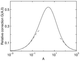
FIG. 1.: The relative temperature correction $G(A,0)$ as a function of the parameter $A$ (20). The other parameter $\tau$ (2) is assumed to be small. The solid curve represents numerical calculation. The dashed lines correspond to the asymptotics (28) and (33).

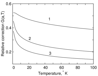
FIG. 2.: The relative temperature correction $G(a,T)$ as a function of temperature at a few values of separations between bodies: (1) $a=100\ nm$, (2) $a=300\ nm$, (3) $a=500\ nm$.

REFERENCES

- [1] H. B. G. Casimir, Proc. K. Ned. Akad. Wet. 51, 793 (1948).
- [2] M. Bordag, U. Mohideen, and V. M. Mostepanenko, Phys. Rep. 353, 1 (2001).
- [3] S. K. Lamoreaux, Phys. Rev. Lett. 78, 5 (1997); 81, 5475 (1998).
- [4] U. Mohideen and A. Roy, Phys. Rev. Lett. 81, 4549 (1998); A. Roy and U. Mohideen, Phys. Rev. Lett. 82, 4380 (1999); A. Roy, C.-Y. Lin, and U. Mohideen, Phys. Rev. D 60, 111101(R) (1999).
- [5] B. W. Harris, F. Chen, and U. Mohideen, Phys. Rev. A 62, 052109 (2000).
- [6] T. Ederth, Phys. Rev. A 62, 062104 (2000).
- [7] H. B. Chan, V. A. Aksyuk, R. N. Kleiman, D. J. Bishop, and F. Capasso, Science, 291, 1941 (2001); Phys. Rev. Lett. 87, 211801 (2001).
- [8] G. Bressi, G. Carugno, R. Onofrio, and G. Ruoso, Phys. Rev. Lett. 88, 041804 (2002).
- [9] S. K. Lamoreaux, Phys. Rev. A 59, R3149 (1999).
- [10] G. L. Klimchitskaya, A. Roy, U. Mohideen, and V. M. Mostepanenko, Phys. Rev. A 60, 3487 (1999).
- [11] M. Boström and Bo E. Sernelius , Phys. Rev. A 61, 046101 (2000).
- [12] A. Lambrecht and S. Reynaud, Eur. Phys. J. D 8, 309 (2000); Phys. Rev. Lett. 84, 5672 (2000).
- [13] V. B. Svetovoy and M. V. Lokhanin, Mod. Phys. Lett. A 15, 1013 (2000).
- [14] G. L. Klimchitskaya, U. Mohideen, and V. M. Mostepanenko, Phys. Rev. A 61, 062107 (2000).
- [15] V. B. Svetovoy and M. V. Lokhanin, Mod. Phys. Lett. A 15, 1437 (2000).
- [16] M. Boström and Bo E. Sernelius, Phys. Rev. Lett. 84, 4757 (2000).
- [17] M. Bordag, B. Geyer, G. L. Klimchitskaya, and V. M. Mostepanenko, Phys. Rev. Lett. 85, 503 (2000).
- [18] C. Genet, A. Lambrecht, and S. Reynaud, Phys. Rev. A 62, 012110 (2000).
- [19] V. B. Svetovoy and M. V. Lokhanin, Phys. Lett. A 280, 177 (2001).
- [20] G. L. Klimchitskaya and V. M. Mostepanenko, Phys. Rev. A 63, 062108 (2001).
- [21] S. K. Lamoreaux, Phys. Rev. Lett. 87, 139101 (2001).
- [22] Bo. E. Sernelius, Phys. Rev. Lett. 87, 139102 (2001).
- [23] Bo E. Sernelius and M. Boström, Phys. Rev. Lett. 87, 259101 (2001).
- [24] M. Bordag, B. Geyer, G. L. Klimchitskaya, and V. M. Mostepanenko, Phys. Rev. Lett. 87, 259102 (2001).
- [25] J.R. Torgerson and S.K. Lamoreaux, quant-ph/0208042.
- [26] E. M. Lifshitz, Zh. Eksp. Teor. Fiz. 29, 94 (1956), [Sov. Phys. JETP 2, 73 (1956)].
- [27] J. Mehra, Physica (Amsterdam) 37, 145 (1967).
- [28] L. S. Brown and G. J. Maclay, Phys. Rev. 184, 1272 (1969).
- [29] J. Schwinger, L. L. DeRaad, Jr., and K. A. Milton, Ann. Phys. (N.Y.) 115, 1 (1978).
- [30] V. B. Bezerra, G. L. Klimchtskaya, and V. M. Mostepanenko, Phys. Rev. A 65, 052113 (2002).
- [31] E. M. Lifshitz and L. P. Pitaevskii, Statistical Physics, Part 2 (Pergamon Press, Oxford, 1980).
- [32] A. A. Abrikosov, Fundamentals of the Theory of Metals (North-Holland, 1988).
- [33] E. M. Lifshitz and L. P. Pitaevskii, Physical Kinetics (Pergamon Press, Oxford, 1981).
- [34] L. D. Landau and E. M. Lifshitz, Electrodynamics of Continuous Media (Pergamon Press, Oxford, 1984).
- [35] V. M. Mostepanenko and N. N. Trunov, Sov. J. Nucl. Phys. (USA) 42, 818 (1985).
- [36] V. B. Bezerra, G. L. Klimchtskaya, and C. Romero, Phys. Rev. A (2002).
- [37] V. M. Mostepanenko and N. N. Trunov, The Casimir Effect and Its Applications (Clarendon, Oxford, 1997).
- [38] I. E. Dzyaloshinskii, E. M. Lifshitz, and L. P. Pitaevskii, Usp. Fiz. Nauk 73, 381 (1961), [Sov. Phys. Usp. 4, 153 (1961)].