Anisotropic velocity distributions in 3D dissipative optical lattices

Abstract

We present a direct measurement of velocity distributions in two dimensions by using an absorption imaging technique in a 3D near resonant optical lattice. The results show a clear difference in the velocity distributions for the different directions. The experimental results are compared with a numerical 3D semi-classical Monte-Carlo simulation. The numerical simulations are in good qualitative agreement with the experimental results.

1 Introduction

An optical lattice is a periodic optical light shift potential created by the interference of laser beams in which atoms can be trapped. Usually one distinguish between two types of lattices, near-resonance optical lattices (NROL) mennerat02 and far-off resonance lattices (FOROL). In the later type, an atom can only be trapped, whereas the former (the one considered in this paper) also exhibits an inherent cooling mechanism (Sisyphus cooling). The Sisyphus cooling mechanism in an NROL has been the subject of extensive research due to its high cooling efficiency, but also since an optical lattice is a very pure quantum system suitable for fundamental studies of atom-light interaction.

Theoretical studies of the atomic motion in NROLs have been done in 1D and 2D, both analytically and numerically. The extension to 3D configurations is however cumbersome. Analytical solutions become unwieldy and numerical simulations require long computation time, especially for high angular momentum transitions. Thus very few detailed studies have been made in 3D. An exception is the work by Castin and Mølmer molmer95 who studied spatial and momentum localization via full quantum Monte Carlo wavefunction simulations in the case of optical molasses.

Measurements of temperature have been made on 3D NROLs by our group ellmann ; jersblad , and by groups at NIST gatzke and in Paris mennerat . In all these experiments, and in this work, the kinetic temperature is derived from measured velocity distributions along one axis and is defined as a direct measure of the kinetic energy through

$$T=\frac{M\langle v^{2}\rangle}{k_{\textrm{\scriptsize B}}},$$ (1)

where $\langle v^{2}\rangle$ is the mean square velocity of the released atoms, $k_{\textrm{\scriptsize B}}$ is the Boltzmann constant and $M$ is the atomic mass. A robust result in all studies is that the temperature scales linearly with the irradiance divided by the detuning, that is linearly with the light shift at the bottom of the optical potential ($U$). This is in excellent qualitative agreement with 1D-theoretical predictions dalibard .

Nevertheless, in several works (for example ellmann , gatzke and this work) a four laser beam configuration results in a face centered tetragonal lattice that cannot simply be reduced to three 1D cases. Indeed, all spatial directions are not equivalent (see section 2.1) and the particular geometry of the lattice has to be taken into account. In a recent paper by the Grynberg group carminati , the dependence of temperature and spatial diffusion on geometric parameters controlling the lattice spatial periods (lattice constants) in different directions was studied. For different laser beam configurations producing the NROL, the temperature and spatial diffusion coefficient were measured for tetragonal lattices (see section 2.1) with different aspect ratios, i.e. as a function of lattice constants. It was shown that the spatial diffusion coefficient strongly depends on the direction. The temperature, which was measured in one direction, was found to be independent of the lattice spacing. The difference between spatial directions lies not only in the lattice constants, but also in the modulations of the laser-atom interaction parameters (optical potentials and optical pumping) in such a way that different behaviors of the temperature along different axes is possible. In palencia the Sisyphus cooling effect in a 3D tetragonal NROL was studied theoretically. With a simplified choice of atomic angular momentum, it was shown by a semi-classical Monte-Carlo calculation that the temperature along a given coordinate axis is independent of the lattice constant, but indeed different along different directions. For the same geometry as considered here, the linear scaling parameter of the temperature differs by a factor of 1.4. Moreover, a comparison between ellmann and gatzke suggests such an anisotropy of the velocity distribution. In both experiments, the direction of measurement coincided with the direction of gravity, but this direction did not correspond to the same lattice axis. It turns out that these works yield a quantitative discrepancy. The derived temperature was found to be linear with $U$ with proportionality constants of 12 nK/$E_{\textrm{{\scriptsize R}}}$ and 24 nK/$E_{\textrm{\scriptsize R}}$ (in ellmann and gatzke respectively), where $E_{\textrm{\scriptsize R}}$ is the recoil energy . The difference in scaling factor called out for a more thorough investigation, which would rule out any systematic error.

This work aims at a direct comparison between the kinetic temperatures along different directions in a 3D NROL. Measurements of velocity distributions along different directions were made for different lattice parameters (potential depth and detuning) by absorption imaging of an expanding atomic cloud. The experimental results are compared with a 3D semi-classical Monte-Carlo simulation performed for the actual atomic angular momentum.

The paper is organized as follows. In section 2.1 we describe the experimental set-up. The experimental data is presented with derived kinetic temperatures in section 2.2. In section 3, we describe the numerical calculation and present the result for the kinetic temperatures. In section 4 we discuss the results from the experiment and the simulations. Finally, in section 5 we draw conclusions on our work.

2 Experiment

2.1 Experimental setup

Initially, a magneto-optical trap (MOT) is loaded with ${N}\approx 2\cdot 10^{6}$ cesium atoms (¹³³Cs) from a chirped decelerated atomic beam in 4 s. This gives a peak number density of $n_{0}\approx 5\cdot 10^{10}$ cm^-3. The MOT operates at the $({F}_{\textrm{g}}=4\rightarrow{F}_{\textrm{e}}=5)$ transition at 852 nm (the D2 line), where $F$ is the total angular momentum quantum number. Due to off-resonant excitation to $F_{\textrm{e}}=4$, a repumper beam resonant with the ($F_{\textrm{g}}=3\rightarrow{F}_{\textrm{e}}=4$) transition is also used. After turning off the loading, the atoms are further cooled in an optical molasses for about 20 ms. From the optical molasses, an atomic cloud at a temperature of $T=3$ $\mu$K is loaded into the optical lattice with a transfer efficiency of about 50%. The filling factor of the lattice is around 0.2 %. The optical lattice beams are red detuned from the $({F}_{\textrm{g}}=4\rightarrow{F}_{\textrm{e}}=5)$ resonance, typically between $\Delta_{5}=-10\Gamma$ and $\Delta_{5}=-40\Gamma$, where $\Gamma/2\pi=5.2$ MHz is the natural linewidth. The atoms equilibrate in the lattice for 10 ms and are then released by turning off the optical lattice beams, with an acousto-optical modulator (AOM) in less than $1{\mu}s$, followed by a measurement of the kinetic temperature. This short falltime of the AOM avoids adiabatic release of the atoms in the optical lattice.

The optical lattice is a 3D generalization of the 1D lin$\perp$lin configuration created by two orthogonally polarized pairs of laser beams that propagate in the yz- and xz-planes respectively mennerat02 . The angle between the beams of each pair is $90^{\circ}$, and each beam forms an angle of $\theta=45^{\circ}$ with the (vertical) quantization (z-) axis (see figure 1). This results in a tetragonal structure with alternating sites of pure $\sigma^{+}$- and $\sigma^{-}$-light, where potential minima are formed. From figure 1, it is clear that directions x and y are equivalent but that direction z is different. It follows that the optical pumping rates and the light shift modulations are different along z compared to x or y. In figure 2 we plot the projection along x and z of the lowest adiabatic potential , which is where the atoms spend most of their time mennerat02 . Two main anisotropic properties arise. First, the lattice constants $a_{z}=\lambda/(2\sqrt{2})$ and $a_{x,y}=\lambda/\sqrt{2}$ are different. Second, the shapes of the potentials are also clearly different. In particular, they show different potential barriers to escape adiabatically from a potential well (lower along the z-direction than what it is along the x- and y-directions by a factor of 1.65) and show different reduced oscillating frequencies ($\omega_{i}a_{i}/\lambda$) at the bottom of the potential wells.

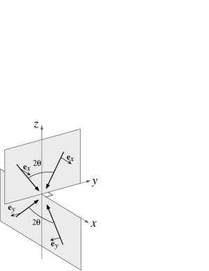
Figure 1: Beam configuration of the 3D lin $\perp$ lin optical lattice. Two beam pairs in the $xz$- and $yz$-planes respectively, orthogonally polarized along the $y$- and $x$-axes respectively, make an angle $\theta=45^{\circ}$ with the $z$-axis.

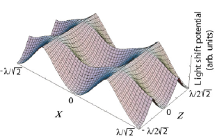
Figure 2: Lowest adiabatic optical lightshift potential projected in the $xz$-plane in units of the optical wavelength, $\lambda$.

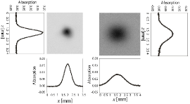
Figure 3: Typical 2D density profiles acquired at two different times $\tau$ after releasing the atoms from the lattice. The left image shows an atomic cloud after $\tau=12.8$ ms expansion together with density profiles in the $z$- and $x$-directions. The right image shows an atomic cloud after $\tau=36.8$ ms.

The velocity distributions along the z- and x-axes are measured using a well known absorption imaging technique walhout . After release from the lattice, a short (50 $\mu$s) resonant probe pulse $(F_{\textrm{g}}=4\rightarrow{F}_{\textrm{e}}=5)$ hits the atomic cloud. The irradiance of the probe pulse is $I\ll I_{0}$, where $I_{0}=1.1$ mW/cm² is the saturation irradiance. The shadow in the probe beam is imaged onto a CCD camera. By capturing images at different time delays after turning off the optical lattice beams, we extract the different spatial density distributions from which velocity distributions can be derived. The velocity distribution in the z-direction (direction of gravity) was compared to the results obtained with a ”time-of-flight” (TOF) method lett , showing good agreement.

2.2 Measured Kinetic Temperatures

The 2D projection (in the xz-plane) of the expanding cloud is recorded at two different time delays, $\tau_{1,2}$, after extinction of the optical lattice beams. Typical values are $\tau_{1}$ = 12 ms and $\tau_{2}$ = 35 ms. Examples of 2D density profiles are shown in figure 3 together with Gaussian fits to the spatial density profile along x and z. Excellent agreement with Gaussian distributions is found. From the fits, we extract the rms radius, $\sigma_{i}$, ($i=x,z$), of the clouds which increases with time, $t$, according to $\sigma_{i}^{2}(t)=\sigma_{i}^{2}(0)+v_{i}^{2}t^{2}$ weiss .

The kinetic temperature in different directions is defined as

$$T_{i}=\frac{M}{k_{\textrm{\scriptsize B}}}\frac{\sigma_{i}^{2}(\tau_{2})-\sigma_{i}^{2}(\tau_{1})}{\tau_{2}^{2}-\tau_{1}^{2}}.$$ (2)

In figure 4 we plot derived kinetic temperatures along x and z for three different detunings, as a function of $U_{0}$, which is the modulation depth of the diabatic optical potential. Here, $U_{0}$ is defined as

$$U_{0}=\frac{\hbar|\Delta_{5}|}{2}\ln\left[1+{\left(\frac{44}{45}\right)\frac{\Omega^{2}}{2\Delta_{5}^{2}}}\right],$$ (3)

where $\Omega^{2}=(\Gamma^{2}/2)/(I/I_{0})$ is the square of Rabi frequency and the irradiance is $I=8I_{\textrm{\scriptsize beam}}$ ($I_{\textrm{\scriptsize beam}}$ is the irradiance of a single beam), at the center of a potential well. For sufficiently high irradiances and temperatures, it is obvious that the universal scaling with $U_{0}$ prevails for each direction. However, this scaling with $U_{0}$ is clearly different for different directions. For large $U_{0}$, the temperature along z is found to be significantly smaller than the temperature along x. Linear fits to the data yield

$$T_{x}=\left(0.55+0.022({U_{0}}/{E_{\textrm{R}}})\right) \mu\textrm{K}$$ (4)

$$T_{z}=\left(0.62+0.012({U_{0}}/{E_{\textrm{R}}})\right) \mu\textrm{K}.$$ (5)

That is, the ratio between the scaling parameters along x and z is determined to be 1.8 (0.3). However, at low modulation depths and low temperatures, the temperatures are found to be approximately the same along z and x.

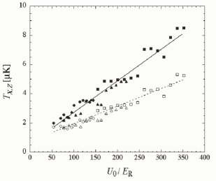
Figure 4: $T_{x}$ (filled) and $T_{z}$ (open) as a function of modulation depth, $U_{0}/E_{R}$, for three different detunings ($\Delta_{5}=-10\Gamma$ (squares) , $-20\Gamma$ (triangles), $-30\Gamma$ (circles)). The solid and dashed line are linear fits to the data.

3 Numerical Simulations

3.1 Theoretical framework

We have performed semi-classical Monte-Carlo simulations in 3D for the actual $(F_{\textrm{g}}=4\rightarrow{F}_{\textrm{e}}=5)$ transition of ¹³³Cs. The main features of the method have been discussed elsewhere palencia ; petsas99 so here we just recall the main elements and peculiarities for our multidimensional configuration.

The optical Bloch equations (OBE), which describe the evolution of a sample of two-level atoms (with Zeeman degeneracy) coupled to both laser fields and vacuum modes, are the starting point of the analysis. Because of the cooling effects and the decoherence due to photon scattering, the atomic cloud dynamics can be reduced to a semi-classical picture for a large range of lattice parameters cohen90 . The OBE are therefore converted into a set of coupled semi-classical Fokker-Planck equations (FPE) via Wigner transforms. Projecting the FPE onto the position-dependent adiabatic states base $|\Phi_{m}(\mathbf{r})\rangle$ (see appendix A) and neglecting the coherence terms which are unimportant in a semi-classical description, one gets a new set of FPE only involving the local populations of the adiabatic states.

By physical interpretation of the FPE, it follows that the atomic cloud dynamics can be reduced to internal state transitions via optical pumping at a rate $\gamma_{n,m}$ from $|\Phi_{n}\rangle$ to $|\Phi_{m}\rangle$, and the evolution of each atom in a given internal $|\Phi_{m}\rangle$-state due to deterministic forces. These forces are first of all due to the optical potential modulation (-$\nabla$$U_{m}$) and secondly, due to the radiation pressure force ($\mathbf{F}$). Moreover, the atomic cloud undergoes momentum diffusion due to photon scattering.

It is then straightforward to show that the FPE solution is formally equivalent to the integration of a set of Langevin equations interrupted by internal states quantum jumps, each one accounting for the random trajectory of a single atom. The quantum jumps are taken into account by generating a random number $r$ at each time step which is compared to the transition probability $\gamma_{m,n}\textrm{d}t$ from $|\Phi_{m}\rangle$ to $|\Phi_{n}\rangle$ (with $n\neq m$) during the time step d$t$. In the following, we define $r_{n,m}$ as $1$ if a quantum jump occurs from $n$ to $m$ and $0$ otherwise. Between two quantum jumps, the elementary evolution of the atom is

$$\textrm{d}\mathbf{R}\left(t\right) = \frac{\mathbf{P}\left(t\right)}{M}\textrm{d}t$$ (6)

$$\textrm{d}\mathbf{P}\left(t\right) = -\mbox{\boldmath$\nabla$}U_{m}\textrm{d}t+\sum_{n\neq m}r_{n,m}\left(\mathbf{\delta p}_{n,m}+\mathbf{F}_{n,m}\textrm{d}t\right)$$ (7)

$$+\big{(}1-\sum_{n\neq m}r_{n,m}\big{)}\left(\mathbf{f}_{m}+\mathbf{F}_{m,m}\right)\textrm{d}t,$$

where $\mathbf{R}$ and $\mathbf{P}$ are the atomic position and momentum respectively. The Hamiltonian force, (-$\nabla$$U_{m}$), is derived from the adiabatic potential in state $|\Phi_{m}\rangle$, and $\mathbf{F}_{n,m}$ is the average radiation pressure in case of a quantum jump from $n$ to $m$ (if $m=n$, no jump occurs). The momentum diffusion is determined by random values: the momentum kick undergone by the atom in case of a quantum jump from $n$ to $m$, $\mathbf{\delta p}_{n,m}$ and the recoil mean force in the absence of a quantum jump, $\mathbf{f}_{m}$. Note that $\mathbf{\delta p}_{n,m}$ and $\mathbf{f}_{m}$ are related to the position-dependent coefficients appearing within the FPE. In a (${\mu}$-indexed) space base where the momentum diffusion matrix $\{D_{n,m}\}$ (see appendix B) is diagonal, the first two moments of $\mathbf{f}_{m}$ and $\mathbf{\delta p}_{n,m}$ read

$$\langle f_{m}^{\mu}\rangle=0 \langle(f_{m}^{\mu})^{2}\rangle=\frac{2D_{m,m}^{\mu,\mu}\left(\mathbf{r}\right)}{dt}$$ and

$$\langle\delta p_{n,m}^{\mu}\rangle=0 \langle(\delta p_{n,m}^{\mu})^{2}\rangle=\frac{2D_{n,m}^{\mu,\mu}\left(\mathbf{r}\right)}{\gamma_{n,m}}.$$ and (8)

3.2 Numerical results

The numerical simulations are performed for a typical sample of $300$ independent atoms. For the lattice parameters considered in this work, the kinetic energy reaches steady-state in a time of approximately $4000/\Gamma^{{}^{\prime}}$, where $\Gamma^{{}^{\prime}}=\Gamma s_{0}/2$ is the total scattering rate and $s_{0}$ is the saturation parameter (see appendix A). The averages of the kinetic energies in steady state in the $x$-, $y$- and $z$-directions provide the kinetic temperatures in the corresponding directions,

$$T_{i}=\frac{M\langle v_{i}^{2}\rangle}{k_{\textrm{\scriptsize B}}}.$$ (9)

The simulations were made for three different detunings ($\Delta_{5}=-10\Gamma,-20\Gamma,-30\Gamma$). For each detuning we acquired velocity distributions, in each direction, at six different modulation depths. Note that the chosen modulation depths are much higher than in the experiment since the semi-classical model breaks down when the momentum distribution becomes too narrow. This is because deep modulation depths are required to avoid non-adiabatic motional couplings between adiabatic sublevels that are not included in our treatment petsas99 . Moreover, the time to reach steady state increases for low modulation depths. However, the linear scaling should still hold. The results of the numerical simulations are shown in figure 5. Here, the kinetic temperature is plotted as a function of modulation depth for the detunings mentioned above. The temperature scales linearly with the light shift independently of the detuning according to

$$T_{x}\propto 0.035(U_{\textrm{\scriptsize 0}}/E_{\textrm{\scriptsize R}}) \mu\textrm{K}$$ (10)

$$T_{y}\propto 0.035(U_{\textrm{\scriptsize 0}}/E_{\textrm{\scriptsize R}}) \mu\textrm{K}$$ (11)

$$T_{z}\propto 0.013(U_{\textrm{\scriptsize 0}}/E_{\textrm{\scriptsize R}}) \mu\textrm{K}$$ (12)

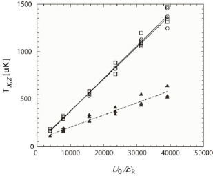
Figure 5: Kinetic temperature, along the $x$- (circles), $y$- (squares) and $z$-direction (filled triangles) as a function of modulation depth, $U_{\textrm{\scriptsize 0}}/E_{\textrm{\scriptsize R}}$, for three different detunings ($\Delta_{5}=-10\Gamma,-20\Gamma,-30\Gamma$). The solid and dashed lines are linear fits to the data.

As in the experiments, the results of the simulations show a clear difference in scaling of the kinetic temperature along the z-axis compared to the x- and y-axes, here, by a factor of 2.7.

4 Discussion

The results from the experimental work and the numerical simulations are compiled in table 1. A comparison shows a quantitative excellent agreement between our experiments and former studies in which the kinetic temperature was measured along x gatzke or along z ellmann . The numerical simulations also reproduce the difference in scaling parameter for different directions was measured in the experiments, and confirms the appearance of a discrepancy between kinetic temperatures along x-y and z.

Table 1: The scaling parameter $\xi_{x,y,z}$, (in units of nK/$E_{\textrm{R}}$), in the equation $T_{x,y,z}=T_{0}+\xi_{x,y,z}U_{0}$ for different studies. The experimental errors of the slope for this work is the quadratic sum of the statistical error and an estimated maximum systematical error. The errors in the simulation is the statistical error from the fit.

	ref ellmann	ref gatzke	this work	this work
			(experimental)	(simulations)
$\xi_{x}$	-	24(2.4)	22(3.5)	35(1.2)
$\xi_{y}$	-	-	-	35(1.2)
$\xi_{z}$	12(1.2)	-	12(2.5)	13(1.0)

The inherent cooling process in an optical lattice for atoms with kinetic energy $E_{\textrm{{\scriptsize K}}}>U_{0}$ is Sisyphus cooling. This process was explained by Dalibard and Cohen-Tannoudji in dalibard in the case of a theoretical transition $(J_{g}=1/2\rightarrow J_{e}=3/2$). The Sisyphus cooling cycle occurs until the atomic kinetic energy is lower than the potential barrier in a particular direction and thus does not depend on any other anisotropy (the lattice spacings for example).

However, for higher angular momentum transitions, the cooling process does not stop because other relaxation processes than standard Sisyphus cooling could still occur petsas99 ; deutsch . For example, atoms in bound states within a lattice well can be excited to unbound states, followed by decay to lower lying vibrational states. We find that the atomic kinetic energy is $E_{\textrm{\scriptsize K}}\sim U_{0}/10$ and thus that the atoms are very well localized at the bottom of the lattice wells in agreement with former experimental investigations, for instance gatzke , and full quantum Monte-Carlo simulations molmer95 . The difference in the scaling factors is proportional to the difference in the modulation depth of the lowest adiabatic optical potential in the corresponding directions. Therefore we conclude that it is this difference which induce anisotropic kinetic temperatures in the optical lattice. This conclusion is not incompatible with the results of carminati in which the steady-state kinetic temperature was measured for different lattice constants showing that the steady-state kinetic temperature was independent of the lattice spacing, because the geometrical anisotropy in the lattice do not reduce to a simple scaling factor between directions x,y and z.

At low modulation depths, the lattice reaches a minimum temperature followed by a sharp increase in temperature, usually called décrochage. When laser cooling is still effective there exists a region where the temperature is isotropic. However, this region is difficult to analyze for several reasons. For instance, at low modulation depths the atomic localization in a trapping site is less strong, and thus the anharmonicity of the potential well becomes more important. This could lead to an increased coupling between the different motional directions and also a broadening of the vibrational levels, i.e. increasing the tunneling rate in the lattice. Another effect that must be taken into account at low modulation depths is increased spatial diffusion carminati ; hodapp . This means that the loss rate of the atoms in the lattice becomes larger, and thus the signal-to-noise in the absorption images decreases. Furthermore, if the thermal expansion of the atomic cloud in the recorded absorption images is small compared to the size of the cloud, due to spatial diffusion, there will be large uncertainties in the extracted temperatures.

5 Conclusions

We have measured the velocity distributions in a 3D optical lattice of cesium along two non-equivalent directions as a function of lightshift ($U_{0}$). In agreement with previous works, the kinetic temperature scales linearly with $U_{0}$. As an original result, we have found that the distributions are clearly anisotropic (with $T_{x,y}>T_{z}$). The experimental results are in good agreement with a 3D numerical Monte-Carlo simulation and we conclude that it is the modulation depth of the adiabatic optical potential that determines the steady-state kinetic temperatures. The anisotropy in kinetic temperature is not paradoxical. In fact the ”kinetic temperature” here is defined as a simple measure of the atomic kinetic energy (see Eq. (1)) and not as a thermodynamical temperature. This is because thermalization in Sisyphus cooling do not result from energy exchange beetween particles via collisions, but from atom-photon interactions. Our result show that no thermodynamical temperature can be defined for Sisyphus cooled atomic samples because of the violation of the equipartition theorem landau80 . Our results can give important clues for a full understanding of the cooling mechanism in an optical lattice. Furthermore, knowledge about the velocity distributions in all directions is important in precision experiments utilizing optical lattices.

Appendix A Optical Bloch equations and adiabatic states

This appendix aims at introducing the adiabatic states for a general $J\rightarrow J+1$ transition atomic sample. Consider an atom of dipole operator $\widehat{\mathbf{D}}=\mathcal{D}(\widehat{\mathbf{d}}^{+}+\widehat{\mathbf{d}}^{-})$ , with $\widehat{\mathbf{d}}^{\pm}$ being the raising and lowering components of $\widehat{\mathbf{D}}$, and $\mathcal{D}$ the reduced dipole moment. This atom interacts with the laser field

$$\mathbf{E}_{\textrm{\scriptsize L}}\left(\mathbf{r},t\right)=\frac{E_{0}}{2}\mathbf{\epsilon}\left(\mathbf{r}\right)e^{-i\omega_{\textrm{\tiny L}}t}+c.c.$$ (13)

, where $E_{0}$ is the amplitude of the electric field, $\omega_{\textrm{\scriptsize L}}$ is the laser frequency and $\mathbf{\epsilon}(\mathbf{r})$ is a vector describing the spatial varying profile of the laser polarization. The operators $\widehat{A}$ and $\widehat{B}_{q}$ represent the hermitian conjugates of the optical pumping cycles (absorption of laser photons followed by emission of stimulated or spontaneous photons respectively), and are defined as

$$\widehat{A}\phantom{{}_{q}}=\left[\widehat{\mathbf{d}}^{-}\cdot\mathbf{\epsilon}^{*}(\mathbf{r})\right]\cdot\left[\widehat{\mathbf{d}}^{+}\cdot\mathbf{\epsilon}(\mathbf{r})\right]$$

$$\widehat{B}_{q}=\left[\widehat{\mathbf{d}}^{-}\cdot\mathbf{\epsilon}^{*}(\mathbf{r})\right]\cdot\left[\widehat{\mathbf{d}}^{+}\cdot\mathbf{e}_{q}\right]$$ (14)

$$\textrm{with }q=0,\pm\phantom{a}\textrm{or }q=x,y,z$$ (15)

where

$$\mathbf{e}_{\pm}=\frac{\mp\mathbf{e}_{x}-i\mathbf{e}_{y}}{\sqrt{2}}\phantom{aaa}\textrm{and}\phantom{aaa}\mathbf{e}_{0}=\mathbf{e}_{z}$$ (16)

are the circular basis vectors. After elimination of the excited state in the low saturation regime,

$$s_{0}=\frac{\Omega^{2}/2}{\Delta^{2}+\Gamma^{2}/4}\ll 1,$$ (17)

the atomic sample dynamics is governed by the OBE involving the projection of the density matrix onto the internal state including an Hamiltonian part:

$$\widehat{H}=\frac{\widehat{\mathbf{p}}^{2}}{2M}+\hbar\frac{\Delta s_{0}}{2}\widehat{A}\left(\mathbf{r}\right)$$ (18)

plus a relaxation part. In the semi-classical limit, the position-dependent adiabatic states are defined as the eigen-states of the light-shift operator $\hbar\frac{\Delta s_{0}}{2}\widehat{A}$:

$$\hbar\frac{\Delta s_{0}}{2}\widehat{A}\left(\mathbf{r}\right)|\Phi_{m}\left(\mathbf{r}\right)\rangle=U_{m}\left(\mathbf{r}\right)|\Phi_{m}\left(\mathbf{r}\right)\rangle.$$ (19)

Note that in general $|\Phi_{m}\left(\mathbf{r}\right)\rangle$ and $U_{m}\left(\mathbf{r}\right)$ cannot be calculated analytically.

Appendix B Dynamics coefficients for the Langevin equation

In this appendix, we give the general expressions for the dynamics coefficients involved in the FPE and Langevin equations for Sisyphus cooling in the low saturation and semi-classical regime. The transition rate from state $|\Phi_{n}\rangle$ to state $|\Phi_{m}\rangle$ (for $m\neq n$) is

$$\gamma_{n,m}=\Gamma_{0}^{\prime}\sum_{q=\pm,0}|\langle\Phi_{n}|\widehat{B}_{q}|\Phi_{m}\rangle|^{2}.$$ (20)

The average radiation pressure term in the direction i (i$=x,y,z$) is

$$F_{n,m}^{i}=-\hbar\Gamma_{0}^{\prime}\;\mathrm{Im}\left(\sum_{q=\pm,0}\langle\Phi_{m}|\partial_{i}\widehat{B}_{q}^{\dagger}|\Phi_{n}\rangle\langle\Phi_{n}|\widehat{B}_{q}|\Phi_{m}\rangle\right)$$ (21)

and the momentum diffusion matrix is

$$D_{n,m}^{i,j} = \frac{\hbar^{2}\Gamma_{0}^{\prime}}{8}\langle\Phi_{n}|\partial_{i,j}^{2}\widehat{A}|\Phi_{m}\rangle\delta_{n,m}$$ (25)

$$+\frac{\hbar^{2}k^{2}\Gamma_{0}^{\prime}}{4}\delta_{i,j}\sum_{\begin{array}[]{c}\phantom{a}^{u\in{x,y,z}}\\ \phantom{a}^{u\neq i,j}\end{array}}\langle\Phi_{m}|\widehat{B}_{u}^{\dagger}|\Phi_{n}\rangle\langle\Phi_{n}|\widehat{B}_{u}|\Phi_{m}\rangle$$

$$-\frac{\hbar^{2}\Gamma_{0}^{\prime}}{8}\sum_{q=\pm,0}\Big{(}\langle\Phi_{m}|\partial_{i,j}^{2}\widehat{B}_{q}^{\dagger}|\Phi_{n}\rangle\langle\Phi_{n}|\widehat{B}_{q}|\Phi_{m}\rangle$$

$$\phantom{aaaaaaaaaaaa}-\langle\Phi_{m}|\partial_{i}\widehat{B}_{q}^{\dagger}|\Phi_{n}\rangle\langle\Phi_{n}|\partial_{j}\widehat{B}_{q}|\Phi_{m}\rangle$$

$$\phantom{aaaaaaaaaaaa}+c.c.\Big{)}$$

where $\delta_{\alpha,\beta}$ is the Kronecker symbol ($1$ when $\alpha=\beta$ and $0$ else) and $i,j$ denotes the spatial directions $(x,y,z)$. Note that for the sake of simplicity, the spontaneous emission pattern is simplified in a way that the photons are restricted to be emitted only along the $x$-, $y$- and $z$-axes. This approximation is justified because the kinetic energy is expected to be greater than the recoil energy castin94 .

References

- (1) G. Grynberg, C. Robilliard, Phys. Rep. 355, 335 (2001)
- (2) Y. Castin, K. Mølmer, Phys. Rev. Lett. 74, 3772 (1995)
- (3) H.Ellmann, J.Jersblad, A.Kastberg, Eur. Phys. J. D 13, 379 (2001)
- (4) J.Jersblad, H.Ellmann, A.Kastberg, Phys. Rev. A 62, R51401 (2000)
- (5) M. Gatzke, G. Birkl, P. S. Jessen, A. Kastberg, S. L. Rolston, W. D. Phillips, Phys. Rev. A 55, R3987 (1997)
- (6) C. Mennerat-Robilliard, L. Guidoni , K. I. Petsas, P. Verkerk, J.-Y. Courtois, G. Grynberg, Eur. Phys. J. D 1, 33 (1998)
- (7) J. Dalibard, C. Cohen-Tannoudji, J. Opt. Soc. Am. B 6, 2023 (1989)
- (8) F.-R. Carminati, M. Schiavoni, L. Sanchez-Palencia, F. Renzoni, G. Grynberg, Eur. Phys. J. D 17, 249 (2001)
- (9) L. Sanchez-Palencia, P. Horak, G. Grynberg, Eur.Phys. J. D 18, 353 (2002)
- (10) M.S. Walhout, Ph.D. thesis, University of Maryland, 1994
- (11) P. Lett, R. Watts, C. Westbrook, W. Phillips, P. Gould , H. Metcalf, Phys. Rev. Lett. 61, 169 (1998)
- (12) D.S Weiss, E. Riis, Y. Shevy, P. J. Ungar, S. Chu, J. Opt. Soc. Am. B 6, 2072 (1989)
- (13) K. I. Petsas, G. Grynberg, J.-Y. Courtois, Eur. Phys. J. D 6, 29 (1999)
- (14) C. Cohen-Tannoudji, Les Houches summer school of theoretical physics 1990, Session LIII, in Fundamental systems in Quantum Optics, edited by J. Dalibard, J. M. Raimond, J. Zinn-Justin (Elsevier Science Publishers, Amsterdam, 1991)
- (15) I. H. Deutsch, J. Grondalski, P. M. Alsing, Phys. Rev. A 56, R1705 (1997)
- (16) T. W. Hodapp, C. Gerz, C. Furtlehner, C. I. Westbrook, W. D. Phillips, J. Dalibard, Appl. Phys. B 60, 135 (1995)
- (17) L. D. Landau, E. M. Lifschitz, Statistical Physics, 3rd ed., Pergamon Press (Oxford, 1980)
- (18) Y. Castin, K. Berg-Sørensen, J. Dalibard, K. Mølmer, Phys. Rev. A 50, 5092 (1994)