NMR implementation of a quantum scheduling algorithm

1 Introduction

The scheduling algorithm solves the intersection problem, i.e., the problem is to find common elements in two sets. Let Alice and Bob be two distant parties who wish to collaborate on a common task. They each have a schedule listing $N$ slots of time. Their schedules can be represented as two strings if Alice and Bob each have $N$ classical or quantum bits. For each person, a bit in state $1$ denotes a slot that is available, and a qubit in state $0$ denotes a slot that is not available. The intersection problem becomes to find the common 1s in the two strings. Alice and Bob need to exchange information to find the common 1s. The problem is how to reduce the exchanging information [1, 2, 3].

If Alice and Bob exchange classical bits, they will need to exchange $O(N)$ bits. H. Buhrman et al found that Alice and Bob could find the common 1s by exchanging $O(\sqrt{N}\log_{2}N)$ qubits, if they exploited the quantum parallelism [4, 5]. Grover proposed an improved algorithm in theory for the special case in which the string of either Alice or Bob has few 1s [6]. Grover’s theoretical scheme can be described as follows. Assume that there is a $\log_{2}N$ qubit register, by setting $N=2^{n}$, where $n$ is an integer. The register can be transmitted between Alice and Bob. Assume that Alice has $\epsilon N$ 1s in her $N$ bit string, where $\epsilon N\ll N$. For convenience, we assume that Bob also has $\epsilon N$ 1s in his $N$ bit string, and there is a single common 1 in the two strings. Alice encodes the $N$ slots in the register, by applying the Walsh-Hadamard transform (denoted as W) to $|\overline{0}>$, where $|\overline{0}>$ denotes that all qubits in the register lie in state $|0>$. After she repeats $WI_{\overline{0}}WI_{A}$ $m$ times, where $m=\pi\sqrt{1/\epsilon}/4$ [7], the register lies in the superposition corresponding to Alice’s available slots. $I_{A}$ denotes the selective inversion (or suitable inversion) for the basis states corresponding to Alice’s available slots. $I_{\overline{0}}$ denotes the selective inversion for $|\overline{0}>$. The composite transformation used by Alice is denoted by $G$, represented by $G\equiv(WI_{\overline{0}}WI_{A})^{m}W$. According to the generalized quantum search algorithm [8], $(GI_{\overline{0}}G^{-1}I_{B})^{m}G$ transforms $|\overline{0}>$ to the state corresponding to the available slot of the both of Alice and Bob, where $G^{-1}$ denotes the inversion of $G$, and $I_{B}$ denotes the selective inversion for the basis states corresponding to Bob’s available slots.

Alice can carry out $W$, $I_{A}$, and $I_{\overline{0}}$. When she needs $I_{B}$, she must send the register to Bob, who applies $I_{B}$ to the register, and then returns it to Alice. One should notes that the overall state of the register is unaltered during the course of sending [3]. Obviously, the number of times the register needs to be sent to Bob is equal to the number of $I_{B}$ operations.

In the improved scheduling algorithm proposed by Grover, he used the original quantum search algorithm, which is not efficient or invalid at all in some cases [9]. The limits on the search algorithm impose restrictions on the quantum scheduling algorithm. In this paper, we generalize Grover’s improved algorithm by replacing $W$ by a proper unitary operator $U$, and replacing the selective inversions by $\pi/2$ phase rotations, in order to make the quantum scheduling algorithm suitable for more cases. Correspondingly, $I_{\overline{0}}$ is also replaced by a $\pi/2$ phase rotation for $|\overline{0}>$. We implement our scheme using nuclear magnetic resonance (NMR).

2 Generalizing the quantum scheduling algorithm

Our experiments use a sample of carbon-13 labelled chloroform dissolved in d6-acetone. Data are taken at room temperature with a Bruker DRX 500 MHz spectrometer. The resonance frequencies $\nu_{1}=125.76$ MHz for ${}^{13}C$, and $\nu_{2}=500.13$ MHz for ${}^{1}H$. The coupling constant $J$ is measured to be 215 Hz. The Hamiltonian of this system is represented as [10]

$$H=-2\pi\nu_{1}I_{z}^{1}-2\pi\nu_{2}I_{z}^{2}+2\pi JI_{z}^{1}I_{z}^{2},$$ (1)

by setting $\hbar=1$, where $I_{z}^{k}(k=1,2)$ are the matrices for $z$-component of the angular momentum of the spins. The evolution caused by a radio-frequency (rf) pulse on resonance along $x$ or $-y$ axis is represented as $R_{x}^{k}(\varphi)=e^{i\varphi I_{x}^{k}}$ or $R_{y}^{k}(-\varphi)=e^{-i\varphi I_{y}^{k}}$, with $k$ specifying the affected spin. The pulse used above is denoted by $[\varphi]_{x}^{k}$ or $[-\varphi]_{y}^{k}$. The coupled-spin evolution is denoted as

$$[\tau]=e^{-i2\pi J\tau I_{z}^{1}I_{z}^{2}},$$ (2)

where $\tau$ is evolution time. The pseudo-pure state

$$|00>=\left(\begin{array}[]{c}1\\ 0\\ 0\\ 0\end{array}\right)$$ (3)

is prepared by using spatial averaging [11], where $|0>$ denotes up spin state. The basis states are arrayed as $|00>,|01>,|10>$, $|11>$. In experiments, we exploit rf and gradient pulse sequence to transform the system from the equilibrium state to the state $\rho_{0}=I_{z}^{1}/2+I_{z}^{2}/2+I_{z}^{1}I_{z}^{2}$, where $\rho_{0}$ denotes the deviation density matrix equivalent to $|00>$ [12].

The Walsh-Hadamard transform is replaced by $U=R_{y}^{1}(\pi/2)R_{y}^{2}(-\pi/2)$, which is represented as

$$U=\frac{1}{2}\left(\begin{array}[]{cccc}1&-1&1&-1\\ 1&1&1&1\\ -1&1&1&-1\\ -1&-1&1&1\end{array}\right).$$ (4)

Alice and Bob each have a four bit string, in which the positions of slots are encoded by a two qubit register. The basis states $|00>$, $|01>$, $|10>$, $|11>$ correspond to the first, second, third, and fourth slots, respectively. Assume that Alice’s available slots are the first and the second ones, which correspond to $|00>$, and $|01>$, respectively. $I_{A}$ is replaced by a $\pi/2$ phase rotation [13], represented as

$$I_{A12}^{\frac{\pi}{2}}=\left(\begin{array}[]{cccc}i&0&0&0\\ 0&i&0&0\\ 0&0&1&0\\ 0&0&0&1\end{array}\right).$$ (5)

Considering the phase matching condition [14], $I_{\overline{0}}$ is replaced by

$$I_{\overline{0}}^{\frac{\pi}{2}}=\left(\begin{array}[]{cccc}i&0&0&0\\ 0&1&0&0\\ 0&0&1&0\\ 0&0&0&1\end{array}\right).$$ (6)

We assume that there are three cases for Bob’s available slots: 1) The first and the fourth slots are available; 2) The second and the third slots are available; and 3) The first and the second slots are available. For the three cases, $I_{B}$ is replaced by

$$I_{B14}^{\frac{\pi}{2}}=\left(\begin{array}[]{cccc}i&0&0&0\\ 0&1&0&0\\ 0&0&1&0\\ 0&0&0&i\end{array}\right),$$ (7)

$$I_{B23}^{\frac{\pi}{2}}=\left(\begin{array}[]{cccc}1&0&0&0\\ 0&i&0&0\\ 0&0&i&0\\ 0&0&0&1\end{array}\right),$$ (8)

$$I_{B12}^{\frac{\pi}{2}}=\left(\begin{array}[]{cccc}i&0&0&0\\ 0&i&0&0\\ 0&0&1&0\\ 0&0&0&1\end{array}\right),$$ (9)

respectively. By defining the composite operators $G_{12}\equiv-UI_{\overline{0}}^{\frac{\pi}{2}}U^{-1}I_{A12}^{\frac{\pi}{2}}U$, $Q_{1}\equiv-G_{12}I_{\overline{0}}^{\frac{\pi}{2}}G_{12}^{-1}I_{B14}^{\frac{\pi}{2}}G_{12}$, $Q_{2}\equiv-G_{12}I_{\overline{0}}^{\frac{\pi}{2}}G_{12}^{-1}I_{B23}^{\frac{\pi}{2}}G_{12}$, and $Q_{12}\equiv-G_{12}I_{\overline{0}}^{\frac{\pi}{2}}G_{12}^{-1}I_{B12}^{\frac{\pi}{2}}G_{12}$, we obtain

$$G_{12}|00>=e^{-i\pi/4}(|00>+|01>)/\sqrt{2},$$ (10)

$$Q_{1}|00>=-i|00>,$$ (11)

$$Q_{2}|00>=-i|01>,$$ (12)

$$Q_{12}|00>=e^{-i\pi/4}(|00>+|01>)/\sqrt{2}.$$ (13)

Eq.(11), for example, shows that the register is transmitted between Alice and Bob only one time, and the common slot, which corresponds to $|00>$, is obtained. Similarly, if Alice’s available slots are the third and fourth ones, we replace $I_{A12}^{\frac{\pi}{2}}$ by

$$I_{A34}^{\frac{\pi}{2}}=\left(\begin{array}[]{cccc}1&0&0&0\\ 0&1&0&0\\ 0&0&i&0\\ 0&0&0&i\end{array}\right)$$ (14)

and obtain

$$G_{34}|00>=-e^{-i\pi/4}(|10>+|11>)/\sqrt{2},$$ (15)

where $G_{34}\equiv-UI_{\overline{0}}^{\frac{\pi}{2}}U^{-1}I_{A34}^{\frac{\pi}{2}}U$. We also assume that there are three cases for Bob: 1) The first and the fourth slots are available; 2) The second and the third slots are available; and 3) The third and the fourth slots are available. By defining $Q_{4}\equiv-G_{34}I_{\overline{0}}^{\frac{\pi}{2}}G_{34}^{-1}I_{B14}^{\frac{\pi}{2}}G_{34}$, $Q_{3}\equiv-G_{34}I_{\overline{0}}^{\frac{\pi}{2}}G_{34}^{-1}I_{B23}^{\frac{\pi}{2}}G_{34}$, and $Q_{34}\equiv-G_{34}I_{\overline{0}}^{\frac{\pi}{2}}G_{34}^{-1}I_{B34}^{\frac{\pi}{2}}G_{34}$, we obtain

$$Q_{4}|00>=i|11>,$$ (16)

$$Q_{3}|00>=i|10>,$$ (17)

$$Q_{34}|00>=-e^{-i\pi/4}(|10>+|11>)/\sqrt{2},$$ (18)

where

$$I_{B34}^{\frac{\pi}{2}}=\left(\begin{array}[]{cccc}1&0&0&0\\ 0&1&0&0\\ 0&0&i&0\\ 0&0&0&i\end{array}\right).$$ (19)

The overall phases before wave functions can be ignored.

3 Experimental procedure and results

The coupled-spin evolution described as Eq.(2) is realized by pulse sequence $\tau/2-[\pi]_{x}^{1,2}-\tau/2-[-\pi]_{x}^{1,2}$ [16], where $[\pi]_{x}^{1,2}$ denotes a nonselective pulse (hard pulse), and the symbol $\tau/2$ denotes the evolution caused by the magnetic field for $\tau/2$ when pulses are switched off. $[\pi]_{x}^{1,2}$ pulses are applied in pairs each of which take opposite phases in order to reduce the error accumulation causes by imperfect calibration of $\pi$-pulses [17]. $U$ is realized by $[\pi/2]_{y}^{1}-[-\pi/2]_{y}^{2}$. $I_{A12}^{\frac{\pi}{2}}=R_{y}^{1}(\pi/2)R_{x}^{1}(\pi/2)R_{y}^{1}(-\pi/2)$ (up to an irrelevant overall phase factor), and is realized by $[-\pi/2]_{y}^{1}-[\pi/2]_{x}^{1}-[\pi/2]_{y}^{1}$, noting that the pulses are applied from left to right [18]. $I_{B14}^{\frac{\pi}{2}}=[7/2J]$, $I_{B23}^{\frac{\pi}{2}}=[1/2J]$, and $I_{B12}^{\frac{\pi}{2}}=I_{A12}^{\frac{\pi}{2}}$. By modifying the pulse sequences in Ref. [19, 14], we find $I_{\overline{0}}^{\frac{\pi}{2}}=R_{y}^{1,2}(\pi/2)R_{x}^{1,2}(\pi/4)R_{y}^{1,2}(-\pi/2)[15/4J]$. By optimizing the pulse sequences, we obtain

$G_{12}=-R_{y}^{1}(\pi/2)R_{y}^{1}(\pi/2)R_{x}^{1,2}(\pi/4)R_{y}^{1,2}(-\pi/2)[15/4J]R_{x}^{1}(\pi/2)$, and

$G_{12}^{-1}=-R_{x}^{1}(-\pi/2)[1/4J]R_{y}^{1,2}(\pi/2)R_{x}^{1,2}(-\pi/4)R_{y}^{1}(-\pi/2)R_{y}^{1}(-\pi/2)$.

Similarly, $I_{A34}^{\frac{\pi}{2}}=R_{y}^{1}(\pi/2)R_{x}^{1}(-\pi/2)R_{y}^{1}(-\pi/2)$, and $I_{B34}^{\frac{\pi}{2}}=I_{A34}^{\frac{\pi}{2}}$. $G_{34}$ can be optimized as $G_{34}=-R_{y}^{1}(\pi/2)R_{y}^{1}(\pi/2)R_{x}^{1,2}(\pi/4)R_{y}^{1,2}(-\pi/2)[15/4J]R_{x}^{1}(-\pi/2)$.

The experimental results are represented by the deviation density matrices reconstructed from the spectra recorded through the readout pulses by the technique of state tomography [15]. We first prepare pseudo- pure state $|00>$. The generalized quantum scheduling algorithm starts with $|00>$. $Q_{1}$, $Q_{2}$, and $Q_{12}$ transform $|00>$ into $|00>$, $|01>$, and $(|00>+|01>)/\sqrt{2}$, respectively. Figs.1(a-c) show the experimentally measured deviation density matrices after $Q_{1}$, $Q_{2}$, and $Q_{12}$ are applied to $|00>$, respectively. Figs.1(d-f) show the theoretically expected matrices $|00><00|$, $|01><01|$, and $(|00>+|01>)(<00|+<01|)/2$, respectively. In contrast with the theoretical expectation, for the values of the theoretical non-zero elements, the relative errors of the experimental values in Figs.1 (a) and (b) are less than $12\%$, and the relative errors in Fig.1 (c) are less than $22\%$. The relative errors increase in Fig.1(c) because the theoretical values are only half of those in Figs.1 (a) and (b). The other small elements in Figs.1(a-c) are less than $30\%$. The errors mainly result from the imperfection of pulses, effect of decoherence and inhomogeneity of magnetic field.

4 Conclusion

We have realized the generalized quantum scheduling algorithm on a two qubit NMR quantum computer, and obtained nontrivial results. For each case discussed above, Alice and Bob each have two available slots in their schedules either of which consists of four slots. The original scheduling algorithm does not work in this case, because the original search algorithm is invalid in the case that the number of the marked states is equal to the number of unmarked states. However, using the generalized scheduling algorithm, Alice and Bob can find the common slots by exchanging the register only one time.

5 Acknowledgements

This work was supported by the National Nature Science Foundation of China. We are also grateful to Professor Shouyong Pei of Beijing Normal University for his helpful discussions on the principle of quantum algorithm and also to Dr. Jiangfeng Du of University of Science and Technology of China for his helpful discussions on experiment.

Figure Captions

1. Experimentally measured deviation density matrices shown as Figs.1(a)-(c) and theoretically expected density matrices shown as Figs.1(d)-(f) after the completion of the quantum scheduling algorithm, corresponding to operations $Q_{1}$, $Q_{2}$, and $Q_{12}$, respectively. Only the real component is plotted. The imaginary portion, which is theoretically zero, is found to contribute less than $15\%$ to the experimental results.

1

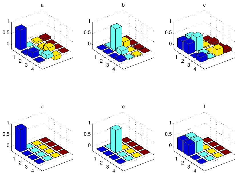
Figure 1:

References

- [1] G. Brassard, quant-ph/0101005
- [2] P. Hyer, R. de Wolf, quant-ph/0109068
- [3] H. Klauck, quant-ph/0005032
- [4] H. Buhrman ,R. Cleve , and A. Wigderson, quant-ph/9802040
- [5] L. K. Grover, Phys. Rev. Lett. 79, 325(1997)
- [6] L. K. Grover, quant-ph/0202033
- [7] Boyer M, Brassard G, Hyer P, and Tapp A, quant-ph/9605034; Fortschr. Phys. 46, 493(1998)
- [8] L. K. Grover, Phys. Rev. Lett, 80, 4329(1998)
- [9] J.-F. Zhang, and Z.-H. Lu, Am. J. Phys, 71, 83(2003)
- [10] R. R. Ernst, G. bodenhausen and A. Wokaum, Principles of nuclear magnegtic resonance in one and two dimensions, (Oxford University Press, New York, 1987)
- [11] D. G. Cory, M. D. Price, and T. F. Havel, Physica D.120,82 (1998)
- [12] J. -F. Zhang, Z. -H. Lu, L. Shan, and Z. -W. Deng, Phys. Rev. A, 65, 034301 (2002)
- [13] E. Biham, O. Biham, D.Biron, M.Grassl, D. A. Lidar, and D. Shapira, Phys. Rev. A, 63, 012310(2000)
- [14] G.-L. Long, H.-Y.Yan, Y.-S.Li, C.-C. Tu, J.-X. Tao, H.-M. Chen, M.-L. Liu, X.Zhang,J.Xiao,X.-Z.Zeng,quant-ph/0009059; Phys. Lett. A, 286,121(2001)
- [15] I. L. Chuang, N. Gershenfeld, M. G. Kubinec and D. W. Leung, Proc. R. Soc. Lond. A 454, 447 (1998)
- [16] N. Linden, . Kupe, and R. Freeman, Chem. Phys. Lett, 311, 321(1999)
- [17] X. Fang, X. Zhu, M. Feng, X. Mao, and F. Du, Phys. Rev. A,61,022307 (2000)
- [18] L. M. K. Vandersypen, M. Steffen, M. H. Sherwood, C. S. Yannoni, G. Bregory, and I. L. Chuang, Appl. Phys. Lett. 76(5), 646(2000)
- [19] I. L. Chuang, N. Gershenfeld, and M. Kubinec. Phys. Rev. Lett. 80, 3408 (1998)