Decoherence-Free Subspaces and Subsystems

Abstract

Decoherence is the phenomenon of non-unitary dynamics that arises as a consequence of coupling between a system and its environment. It has important harmful implications for quantum information processing, and various solutions to the problem have been proposed. Here we provide a detailed a review of the theory of decoherence-free subspaces and subsystems, focusing on their usefulness for preservation of quantum information.

1 Introduction

Recent results indicating that quantum information processing (QIP) is inherently more powerful than its classical counterpart Gruska:book ; Kitaev:book ; Nielsen:book have motivated a resurgence of interest in the problem of decoherence Giulini:book . Decoherence is a consequence of the inevitable coupling of any quantum system to its environment (or bath), causing information loss from the system to this environment. It was recognized early on that decoherence poses a serious obstacle to physical realization of quantum information processors Landauer:95 ; Unruh:95 . Here we define decoherence as non-unitary dynamics that is a consequence of system-environment coupling. This includes (but is not limited to) both dissipative and dephasing contributions, traditionally known as $T_{1}$ and $T_{2}$ processes, respectively. Dissipation refers to processes in which the populations of the quantum states are modified by interactions with the environment, while dephasing refers to processes that randomize the relative phases of the quantum states. Both are caused by entanglement of the system with environmental degrees of freedom, leading to non-unitary system dynamics note1 . For QIP and other forms of quantum control, any such interaction that degrades the unitary nature of the quantum evolution is undesirable, since it causes loss of coherence of the quantum states and hence an inevitable decay of their interference and entanglement. Interference is crucial for coherent control schemes Shapiro:00 ; Rabitz:00 , while entanglement is believed to be as important an ingredient of the quantum computational speed-up Ekert:98 . In fact, a sufficiently decohered quantum computer can be efficiently simulated on a classical computer Aharonov:96a . In this review we provide a detailed introduction to the theory of decoherence-free subspaces and subsystems (DFSs), which have been conceived as one of the possible solutions to decoherence in QIP. Space limitations prevent us from discussing in detail the interesting problem of performing computation using DFSs. Instead we focus here on the use of DFSs as a way to preserve delicate quantum information.

2 Historical Background

Environment-induced decoherence is a very extensively studied phenomenon in the quantum theory of measurement, and of the transition from quantum to classical behavior. Zurek has shown that environmental superselection results in the establishment of certain special states that show redundancies in their correlations with the environment, and that may consequently be essentially unperturbed by this Zurek:81 . These states, referred to as “pointer states” , are defined by a “predictability sieve” Zurek:93 . While analysis of measurements are complicated by the presence of a measurement apparatus in addition to the system and environment, the notion of a special set of states that are defined by some underlying symmetry in the global physical description is a common element. Another noteworthy early study employing symmetries in order to reduce the coupling of subsets of system states to the environment is Alicki’s work on limited thermalization Alicki:88 . Identifying the power of such symmetries in the physical Hamiltonian, and systematizing the way to find such symmetries has been one of the major innovative features of the recent development of DFS theory and its applications for quantum computation.

Early discussions of the effects of decoherence on quantum computation focused on putting conditions on the strength of coupling of the system-environment coupling and on the duration of quantum gates Landauer:95 ; Unruh:95 . The search for systematic ways to bypass decoherence in the context of QIP, based on identification of states that might be immune to certain decohering interactions, started with observations of Palma, Suominen, and Ekert Palma:96 in a study of the effects of pure dephasing, that two qubits possessing identical interactions with the environment do not decohere. Palma et al. used the term “subdecoherence” to describe this phenomenon, suggested using the corresponding states to form a “noiseless” encoding into logical qubits, and noted that the set of states robust against dephasing will depend on the specific form of qubit-environment coupling. This model was subsequently studied using a different method by Duan and Guo Duan:98 , with similar conclusions and a change of terminology to “coherence preserving states”. The idea of pairing qubits as a means for preserving coherence was further generalized by Duan and Guo in Duan:97PRL , where it was shown that both collective dephasing and dissipation could be prevented. However this assumed knowledge of the system-environment coupling strength. These early studies were subsequently cast into a general mathematical framework for DFSs of more general system/environment interactions by Zanardi and Rasetti, first for the spin-boson model in Zanardi:97c , where the important “collective decoherence” model was introduced (where several qubits couple identically to the same environment, while undergoing both dephasing and dissipation), then for general Hamiltonians Zanardi:97a . Their elegant algebraic analysis established the importance of identifying the dynamical symmetries in the system-environment interaction, and provided the first general formal condition for decoherence-free (DF) states, that did not require knowledge of the system-environment coupling strength. In the work of Zanardi and Rasetti these are referred to as “error avoiding codes”. Several papers focusing on collective dissipation appeared subsequently Zanardi:97b ; Duan:98b ; Duan:98c , as well as applications to encoding information in quantum dots Zanardi:98 ; Zanardi:99aa . Zanardi Zanardi:98a and independently Lidar, Chuang, and Whaley Lidar:PRL98 showed that DF states could also be derived from very general considerations of Markovian master equations. Lidar et al. introduced the term “decoherence-free subspace”, analyzed their robustness against perturbations, and pointed out that the absence of decoherence for DF states can be spoiled by evolution under the system Hamiltonian, identifying a second major requirement for viable use of the DF states for either quantum memory or quantum computation Lidar:PRL98 . A completely general condition for the existence of DF states was subsequently provided in terms of the Kraus operator sum representation (OSR) by Lidar, Bacon and Whaley Lidar:PRL99 . All these studies share essentially the same canonical example of system-environment symmetry: A qubit-permutation symmetry in the system-environment coupling, that gives rise to collective dephasing, dissipation, or decoherence. The other main example of a symmetry giving rise to large DFSs was provided by Lidar et al. in Lidar:00a . This is a much weaker form of spatial symmetry than permutation-invariance, termed “multiple-qubit errors”, which we describe in detail in Section 6.4.

Several papers reported various generalizations of DFSs, e.g., by extending DFSs to quantum groups Durdevich:00 , using the rigged Hilbert space formalism Qiao:02a , and deriving DFSs from a scattering S-matrix approach Shapiro:02 . However, the next major step forward in generalizing the DFS concept was taken by Knill, Laflamme, and Viola Knill:99a , who introduced the notion of a “noiseless subsystem”. Whereas previous DFS work had characterized DF states as singlets (one dimensional irreducible representations) of the algebra generating the dynamical symmetry in the system-bath interaction, the work by Knill et al. showed that higher dimensional irreducible representations can support DF states as well. An important consequence was the reduction of the number of qubits needed to construct a DFS under collective decoherence from four to three. This was noted independently by De Filippo DeFilippo:00 and by Yang and Gea-Banacloche Yang:01 . The generalization from subspaces to subsystems has provided a powerful and elegant tool on which the full theory of universal, fault tolerant quantum computation on DF states has now been established Zanardi:99a ; Kempe:00 . It has also provided a basis for unifying essentially all known decoherence-suppression/avoidance strategies Zanardi:99d ; Zanardi:02 . In the remainder of this chapter we shall follow our usual convention to refer to both subsystems and subspaces interchangeably with the acronym DFS, the distinction being made explicit when necessary.

Following the initial studies establishing the conditions for DFSs, Bacon,Lidar, and Whaley made a thorough investigation of the robustness of DF states to symmetry breaking perturbations Bacon:99 . These authors also showed that the passive error correction (“error avoidance”) properties of a DFS can be combined with the active error correction protocols provided by quantum error correction by concatenation of a DFS inside a quantum error correcting code (QECC) Kitaev:book ; Steane:99 , resulting in an encoding capable of protecting against both collective and independent errors Lidar:PRL99 . A combined DFS-QECC method was shown to be necessary in order to be enable universal, fault tolerant quantum computation in the multiple-qubit errors model Lidar:00b . Interestingly, the DFS for collective decoherence offers a natural energy barrier against other decoherence processes, a phenomenon termed “supercoherence” by Bacon, Brown and Whaley Bacon:01 . Several more recent studies, by Alber et al. and Khodjasteh and Lidar, have considered other hybrid DFS-QECC schemes, focusing in particular on protection against spontaneous emission Alber:01 ; Alber:01a ; KhodjastehLidar:02 . DFSs have also been combined with the quantum Zeno effect by Beige et al. Beige:99 ; Beige:00 . Most recently, a combination of DFSs and the method of dynamical decoupling Viola:98 was shown to offer a complete alternative to QECC ByrdLidar:01a ; LidarWu:02 .

These explicit theoretical demonstrations that, firstly, DF states exist and can provide stable quantum memory, and second, that fault tolerant universal computation can be performed on states encoded into a DFS, while initially superficially surprising to many, have generated several experimental searches for verification of DFSs. The first experimental verification came with a demonstration by Kwiat et al. of a 2-qubit DFS protecting photon states against collective dephasing Kwiat:00 . The same 2-qubit DFS was subsequently constructed and verified to reduce decoherence in ion trap experiments by Kielpinski et al. Kielpinski:01 . In the latter experiment an atomic state of one ion was combined with that of a spectator ion to form a 2-ion DF state that was shown to be protected against dephasing deriving from long wavelength ambient magnetic field fluctuations. This experiment is significant in showing the potential of DFS states to protect fragile quantum state information against decoherence operative in current experimental schemes. More recently, universal control on the same 2-qubit DFS for collective dephasing has been demonstrated in the context of liquid state nuclear magnetic resonance by Fortunato et al. Fortunato:01 . Nuclear magnetic resonance has also led to the first experimental demonstration, by Viola et al., of a 3-qubit DF subsystem, providing immunity against full collective decoherence deriving from a combination of collective spin flips and collective dephasing Viola:01b . With these first experimental demonstrations, further experimental efforts towards implementation of DFSs in active quantum computation, or merely as quantum memory encodings to transport single qubits from one position to another without incurring dephasing, seems assured. For example, the use of a DFS has been identified as a major component in the construction of a scalable trapped ion quantum computer Kielpinski:02 ; Brown:02 ; LidarWu:02 .

A common criticism of the theory of DFSs has been that the conditions required for a DFS to exist are very stringent and the assumptions underlying the theory may be too unrealistic. It is important to emphasize that the DFS concept was never meant to provide a full and independent solution to all decoherence problems. Instead, the central idea has been to make use of the dynamical symmetries in the system-environment interaction first (if they exist), and then to consider the next level of protection against decoherence. The robustness properties of DFSs ensure that this is a reasonable approach. In addition, while the experimental evidence to date Kwiat:00 ; Kielpinski:01 ; Viola:01b ; Fortunato:01 ; Fortunato:02 ; Ollerenshaw:02 , is a reason for cautious optimism, there have also been a number of theoretical studies showing that the conditions for DFSs may be created via the use of the dynamical decoupling method, by symmetrizing the system-bath interaction Zanardi:98b ; Viola:00a ; WuLidar:01b ; WuByrdLidar:02 . This holds true for a wide range of system-bath interaction Hamiltonians. It seems quite plausible that such active “environment engineering” methods will be necessary for DFSs to become truly comprehensive tools in the quest to protect fragile quantum information.

In the remainder of this review we will now leave the historical perspective and provide instead a summary of the theory of DF subspaces and their generalizations, DF subsystems. We shall start, in Section 3 with a simple example of DFSs in physical systems that is then used as a basis for a rigorous analysis of decoherence and the conditions for lack of this in an open quantum system (Section 4). We then provide, in Section 5, a series of complementary characterizations of what a DFS is, using both exact and approximate formulations of open systems dynamics. A number of examples of DFSs in different physical systems follow in Section 6, some of them new. The later sections of the review deal with the generalization to DF Subsystems (Section 7), and the robustness of DFSs (Section 8). We conclude in Section 9.

3 A Simple Example of Decoherence-Free Subspaces: Collective Dephasing

Let us begin by analyzing in detail the operation of the simplest DFS. This example, first analyzed by Palma et al. in Palma:96 and generalized by Duan & Guo Duan:98 , will serve to illustrate what is meant by a DFS. Suppose that a system of $K$ qubits (two-level systems) is coupled to a bath in a symmetric way, and undergoes a dephasing process. Namely, qubit $j$ undergoes the transformation

$$|0\rangle_{j}\rightarrow|0\rangle_{j}\qquad|1\rangle_{j}\rightarrow e^{i\phi}|1\rangle_{j},$$ (1)

which puts a random phase $\phi$ between the basis states $|0\rangle$ and $|1\rangle$ (eigenstates of $\sigma_{z}$ with respective eigenvalues $+1$ and $-1$). This can also be described by the matrix $R_{z}(\phi)=\mathrm{diag}\left(1,e^{i\phi}\right)$ acting on the $\{|0\rangle,|1\rangle\}$ basis. We assume that the phase has no space ($j$) dependence, i.e., the dephasing process is invariant under qubit permutations. This symmetry is an example of the more general situation known as “collective decoherence” . Since the errors can be expressed in terms of the single Pauli spin matrix $\sigma_{z}$ of the two-level system, we refer to this example as “weak collective decoherence” . The more general situation when errors involving all three Pauli matrices are present, i.e., dissipation and dephasing, is referred to as “strong collective decoherence” . Without encoding a qubit initially in an arbitrary pure state $|\psi\rangle_{j}=a|0\rangle_{j}+b|1\rangle_{j}$ will decohere. This can be seen by calculating its density matrix as an average over all possible values of $\phi$,

$$\rho_{j}=\int_{-\infty}^{\infty}R_{z}(\phi)|\psi\rangle_{j}\langle\psi|R_{z}^{\dagger}(\phi)\,p(\phi)d\phi,$$

where $p(\phi)$ is a probability density, and we assume the initial state of all qubits to be a product state. For a Gaussian distribution, $p(\phi)=\left(4\pi\alpha\right)^{-1/2}\exp(-\phi^{2}/4\alpha)$, it is simple to check that

$$\rho_{j}=\left(\begin{array}[]{cc}|a|^{2}&ab^{\ast}e^{-\alpha}\\ a^{\ast}be^{-\alpha}&|b|^{2}\end{array}\right).$$

The decay of the off-diagonal elements in the computational basis is a signature of decoherence.

Let us now consider what happens in the two-qubit Hilbert space. The four basis states undergo the transformation

$$|0\rangle_{1}\otimes|0\rangle_{2} \rightarrow |0\rangle_{1}\otimes|0\rangle_{2}$$

$$|0\rangle_{1}\otimes|1\rangle_{2} \rightarrow e^{i\phi}|0\rangle_{1}\otimes|1\rangle_{2}$$

$$|1\rangle_{1}\otimes|0\rangle_{2} \rightarrow e^{i\phi}|1\rangle_{1}\otimes|0\rangle_{2}$$

$$|1\rangle_{1}\otimes|1\rangle_{2} \rightarrow e^{2i\phi}|1\rangle_{1}\otimes|1\rangle_{2}\rangle.$$

Observe that the basis states $|0\rangle_{1}\otimes|1\rangle_{2}$ and $|1\rangle_{1}\otimes|0\rangle_{2}$ acquire the same phase. This suggests that a simple encoding trick can solve the problem. Let us define encoded states by $|0_{L}\rangle=|0\rangle_{1}\otimes|1\rangle_{2}\equiv|01\rangle$ and $|1_{L}\rangle=|10\rangle$. Then the state $|\psi_{L}\rangle=a|0_{L}\rangle+b|1_{L}\rangle$ evolves under the dephasing process as

$$|\psi_{L}\rangle\rightarrow a|0\rangle_{1}\otimes e^{i\phi}|1\rangle_{2}+be^{i\phi}|1\rangle_{1}\otimes|0\rangle_{2}=e^{i\phi}|\psi_{L}\rangle,$$

and the overall phase thus acquired is clearly unimportant. This means that the 2-dimensional subspace $DFS_{2}(0)=\mathrm{Span}\{|01\rangle,|10\rangle\}$ of the 4-dimensional Hilbert space of two qubits is decoherence-free. The subspaces $DFS_{2}(2)=\mathrm{Span}\{|00\rangle\}$ and $DFS_{2}(-2)=\mathrm{Span}\{|11\rangle\}$ are also (trivially) DF, since they each acquire a global phase as well, $1$ and $e^{2i\phi}$ respectively. Since the phases acquired by the different subspaces differ, there is decoherence between the subspaces.

For $K=3$ qubits a similar calculation reveals that the subspaces $DFS_{3}(1)=\mathrm{Span}\{|001\rangle,|010\rangle,|100\rangle\}$ and $DFS_{3}(-1)=\mathrm{Span}\{|011\rangle,|101\rangle,|110\rangle\}$ are DF, as well the (trivial) subspaces $DFS_{3}(3)=\mathrm{Span}\{|000\rangle\}$ and $DFS_{3}(3)=\mathrm{Span}\{|111\rangle\}$.

More generally, let

$$\lambda_{K}=\mathrm{number\ of\ }0^{\prime}\mathrm{s\ minus\ the\ number\ of\ }1^{\prime}\mathrm{s}$$

in a computational basis state (i.e., a bitstring) over $K$ qubits. Then it is easy to check that any subspace spanned by states with constant $\lambda_{K}$ is DF, and can be denoted $DFS_{K}(\lambda_{K})$ in accordance with the notation above. The dimensions of these subspaces are given by the binomial coefficients: $d\equiv\dim[DFS_{K}(\lambda_{K})]={K\choose\lambda_{K}}$ and they each encode $\log_{2}d$ qubits.

The encoding for the “collective phase damping” model discussed here has been tested experimentally. The first-ever experimental implementation of DFSs used the $DFS_{2}(0)$ subspace to protect against artifially induced decoherence in a linear optics setting Kwiat:00 . The same encoding was subsequently used to alleviate the problem of external fluctuating magnetic fields in an ion trap quantum computing experiment Kielpinski:01 , and figures prominently in theoretical constructions of encoded, universal quantum computation LidarWu:01 ; LidarWu:02 ; ByrdLidar:01a .

4 Formal Treatment of Decoherence

Let us now present a more formal treatment of decoherence. Consider a closed quantum system, composed of a system $S$ of interest defined on a Hilbert space $\mathcal{H}$ (e.g., a quantum computer) and a bath $B$. The full Hamiltonian is

$$\mathbf{H}=\mathbf{H}_{S}\otimes\mathbf{I}_{B}+\mathbf{I}_{S}\otimes\mathbf{H}_{B}+\mathbf{H}_{I},$$ (2)

where $\mathbf{H}_{S}$, $\mathbf{H}_{B}$ and $\mathbf{H}_{I}$ are, respectively, the system, bath and system-bath interaction Hamiltonians, and $\mathbf{I}$ is the identity operator. The evolution of the closed system is given by $\rho_{SB}(t)=\mathbf{U}\rho_{SB}(0)\mathbf{U}^{\dagger}$, where $\rho_{SB}$ is the combined system-bath density matrix and the unitary evolution operator is

$$\mathbf{U}=\exp(-i\mathbf{H}t)$$ (3)

(we set $\hbar=1$). Assuming initial decoupling between system and bath, the evolution of the closed system is given by: $\rho_{SB}(t)=\mathbf{U}(t)[\rho_{S}(0)\otimes\rho_{B}(0)]\mathbf{U}^{\dagger}(t)$. Without loss of generality the interaction Hamiltonian can be written as

$$\mathbf{H}_{I}=\sum_{\alpha}\mathbf{S}_{\alpha}\otimes{\ \mathbf{B}}_{\alpha},$$ (4)

where $\mathbf{S}_{\alpha}$ and $\mathbf{B}_{\alpha}$ are, respectively, system and bath operators. It is this coupling between system and bath that causes decoherence in the system, through entanglement with the bath. To see this more clearly it is useful to arrive at a description of the system alone by averaging out the uncontrollable bath degrees of freedom, a procedure formally implemented by performing a partial trace over the bath:

$$\rho(t)={\textrm{Tr}}_{B}[\mathbf{U}(t)\rho(0)\otimes\rho_{B}(0)\mathbf{U}^{\dagger}(t)].$$

The reduced density matrix $\rho(t)$ now describes the system alone. By diagonalizing the initial bath density matrix, $\rho_{B}(0)=\sum_{\nu}\lambda_{\nu}|\nu\rangle\langle\nu|$, and evaluating the partial trace in the same basis one finds:

$$\rho(t) = \sum_{\mu}\langle\mu|\mathbf{U}(t)\left(\rho(0)\otimes\sum_{\nu}\lambda_{\nu}|\nu\rangle\langle\nu|\right)\mathbf{U}^{\dagger}(t)|\mu\rangle$$ (5)

$$= \sum_{a}\mathbf{A}_{a}\,\rho(0)\,\mathbf{A}_{a}^{\dagger},$$

where the “Kraus operators” are given by:

$$\mathbf{A}_{a}=\sqrt{\lambda_{\nu}}\langle\mu|\mathbf{U}|\nu\rangle\;;\qquad a=(\mu,\nu).$$ (6)

The expression (5) is known as the Operator Sum Representation (OSR) and can be derived from an axiomatic approach to quantum mechanics, without reference to Hamiltonians Kraus:83 . Since Tr$\rho(t)=1$ the Kraus operators satisfy the normalization constraint

$$\sum_{a}\mathbf{A}_{a}^{\dagger}\mathbf{A}_{a}=\mathbf{I}_{S}.$$ (7)

Because of this constraint it follows that when the sum in Eq. (5) includes only one term the dynamics is unitary. Thus a simple criterion for decoherence in the OSR is the presence of multiple independent terms in the sum in Eq. (5).

While the OSR is a formally exact description of the dynamics of the system density matrix, its utility is somewhat limited because the explicit calculation of the Kraus operators is equivalent to a full diagonalization of the high-dimensional Hamiltonian $\mathbf{H}$. Furthermore, the OSR is in a sense too strict. This is because as a closed-system formulation it incorporates the possibility that information which is put into the bath will back-react on the system and cause a recurrence. Such interactions will always occur in the closed-system formulation (due to the the Hamiltonian being Hermitian). However, in many practical situations the likelihood of such an event is extremely small. Thus, for example, an excited atom which is in a “cold” bath will radiate a photon and decohere, but the bath will not in turn return the atom back to its excited state, except via the (extremely long) recurrence time of the emission process. In these situations a more appropriate way to describe the evolution of the system is via a quantum dynamical semigroup master equation Lindblad:76 ; Alicki:87 . By assuming that (i) the evolution of the system density matrix is governed by a one-parameter semigroup (Markovian dynamics), (ii) the evolution is futher “completely positive” Alicki:87 , and (iii) the system and bath density matrices are initially decoupled, Lindblad Lindblad:76 has shown that the most general evolution of the system density matrix $\mathbf{\rho}_{S}(t)$ is governed by the master equation

$${\frac{d\mathbf{\rho}(t)}{dt}} = -i[\mathbf{\tilde{H}}_{S},\mathbf{\rho}(t)]+\mathtt{L}_{D}[\mathbf{\rho}(t)]$$

$$\mathtt{L}_{D}[\mathbf{\rho}(t)] = {\frac{1}{2}}\sum_{\alpha,\beta=1}^{M}a_{\alpha\beta}\left([\mathbf{F}_{\alpha},\mathbf{\rho}(t)\mathbf{F}_{\beta}^{\dagger}]+[\mathbf{F}_{\alpha}\mathbf{\rho}(t),\mathbf{F}_{\beta}^{\dagger}]\right)$$ (8)

where $\mathbf{\tilde{H}}_{S}=\mathbf{H}_{S}+\Delta$ is the system Hamiltonian $\mathbf{H}_{S}$ including a possible unitary contribution from the bath $\Delta$ (“Lamb shift” ), the operators $\mathbf{F}_{\alpha}$ constitute a basis for the $M$-dimensional space of all bounded operators acting on $\mathcal{H}$, and $a_{\alpha\beta}$ are the elements of a positive semi-definite Hermitian matrix. The commutator involving $\mathbf{\tilde{H}}_{S}$ is the ordinary, unitary, Heisenberg term. All the non-unitary, decohering dynamics is accounted for by $\mathtt{L}_{D}$, and this is one of the advantages of the Lindblad equation: unlike the OSR, it clearly separates unitary from decohering dynamics. For a derivation of the Lindblad equation from the OSR, using a coarse graining procedure, including an explicit calculation of the coefficients $a_{\alpha\beta}$ and the Lamb shift $\Delta$, see Lidar:CP01 . Note that the $\mathbf{F}_{\alpha}$ can often be identified with the $\mathbf{S}_{\alpha}$ of the interaction Hamiltonian in Eq. (4) Lidar:CP01 .

5 The DFS Conditions

With the above statement of the conditions for decoherence let us now show how to formally eliminate decoherence. It is convenient to do so by reference to the Hamiltonian, OSR, and semigroup formulations. This leads to a number of essentially equivalent formulations of the conditions for DF dynamics, whose utility is determined by the approach one would like to employ to study a specific problem. In addition, it is useful to give formulations which make contact with the theory of quantum error correcting codes (QECC). First, let us give a formal definition of a DFS:

Definition 1

A system with Hilbert space ${\cal H}$ is said to have a decoherence-free subspace $\tilde{{\cal H}}$ if the evolution inside $\tilde{{\cal H}}\subset{\cal H}$ is purely unitary.

Note that because of the possibility of a bath-induced Lamb shift [$\Delta$ in Eq. (8)] this definition of a DFS does not entirely rule out adverse effects a bath may have on a system. Also, we are not excluding unitary errors that may be the result of inaccurate implementation of quantum logic gates. Both of these problems, which in practice are inseparable, must be dealt with by other methods, such as concatenated codes Lidar:PRL99 .

5.1 Hamiltonian Formulation

As remarked above, in terms of the Hamiltonian $\mathbf{H}$ of Eq. (2), decoherence is the result of the entanglement between system and bath caused by the interaction term $\mathbf{H}_{I}$. In other words, if $\mathbf{H}_{I}=0$ then system and bath are decoupled and evolve independently and unitarily under their respective Hamiltonians $\mathbf{H}_{S}$ and $\mathbf{H}_{B}$. Clearly, then, a sufficient condition for decoherence free (DF) dynamics is that $\mathbf{H}_{I}=0$. However, since one cannot simply switch off the system-bath interaction, in order to satisfy this condition it is necessary to look for special subspaces of the full system Hilbert space $\mathcal{H}$. As shown first by Zanardi and Rasetti Zanardi:97a , such a subspace is found by assuming that there exists a set $\{|\tilde{k}\rangle\}$ of eigenvectors of the $\mathbf{S}_{\alpha}$’s with the property that:

$$\mathbf{S}_{\alpha}|\tilde{k}\rangle=c_{\alpha}|\tilde{k}\rangle\qquad\forall\alpha,|\tilde{k}\rangle.$$ (9)

Note that these eigenvectors are degenerate, i.e., the eigenvalue $c_{\alpha}$ depends only on the index $\alpha$ of the system operators, but not on the state index $k$. If $\mathbf{H}_{S}$ leaves the Hilbert subspace $\tilde{\mathcal{H}}=\mathrm{Span}[\{|\tilde{k}\rangle\}]$ invariant, and if we start within $\tilde{\mathcal{H}}$, then the evolution of the system will be DF. To show this we follow the derivation in Lidar:PRL99 : First expand the initial density matrices of the system and the bath in their respective bases: $\rho_{S}(0)=\sum_{ij}s_{ij}|\tilde{\imath}\rangle\langle\tilde{j}|$ and $\rho_{B}(0)=\sum_{\mu\nu}{b}_{\mu\nu}|{\mu}\rangle\langle\nu|$. Using Eq. (9), one can write the combined operation of the bath and interaction Hamiltonians over $\tilde{\mathcal{H}}$ as:

$$\mathbf{I}_{S}\otimes\mathbf{H}_{B}+\mathbf{H}_{I}=\mathbf{I}_{S}\otimes\mathbf{H}_{{\textrm{c}}}\equiv\mathbf{I}_{S}\otimes[\mathbf{H}_{B}+\sum_{\alpha}a_{\alpha}\mathbf{B}_{\alpha}].$$

This clearly commutes with $\mathbf{H}_{S}$ over $\tilde{\mathcal{H}}$. Thus since neither $\mathbf{H}_{S}$ (by our own stipulation) nor the combined Hamiltonian $\mathbf{H}_{\mathrm{c}}$ takes states out of the subspace:

$$\mathbf{U}[|\tilde{\imath}\rangle\otimes|\mu\rangle]=\mathbf{U}_{S}|\tilde{\imath}\rangle\otimes\mathbf{U}_{\mathrm{c}}|\mu\rangle,$$ (10)

where $\mathbf{U}_{S}=\exp(-i\mathbf{H}_{S}t)$ and $\mathbf{U}_{{\textrm{c}}}=\exp(-i\mathbf{H}_{{\textrm{c}}}t)$. Hence it is clear, given the initially decoupled state of the density matrix, that the evolution of the closed system will be: $\rho_{SB}(t)=\sum_{ij}s_{ij}\mathbf{U}_{S}|\tilde{\imath}\rangle\langle\tilde{j}|\mathbf{U}_{S}^{\dagger}\otimes\sum_{\mu\nu}b_{\mu\nu}\mathbf{U}_{\mathrm{c}}|\mu\rangle\langle\nu|\mathbf{U}_{\mathrm{c}}^{\dagger}.$ It follows using simple algebra that after tracing over the bath: $\rho_{S}(t)=\mathrm{Tr}_{B}[\rho_{SB}(t)]=\mathbf{U}_{S}\rho_{S}(0)\mathbf{U}_{S}^{\dagger}$, i.e., that the system evolves in a completely unitary fashion on $\tilde{\mathcal{H}}$: under the condition of Eq. (9) the subspace is DF. As shown in Ref.  Zanardi:97a by performing a short-time expansion, Eq. (10) is also a necessary condition for a DFS. Let us summarize this:

Theorem 5.1

Let the interaction between a system and a bath be given by the Hamiltonian of Eq. (2). If ${\bf H}_{S}$ leaves the Hilbert subspace $\tilde{{\cal H}}={\rm Span}[\{|\tilde{k}\rangle\}]$ invariant, and if we start within $\tilde{{\cal H}}$, then $\tilde{{\cal H}}$ is a DFS if and only if it satisfies Eq. (9).

The condition of Eq. (9) is very useful for checking whether a given interaction supports a DFS: The operators $\mathbf{S}_{\alpha}$ often form a Lie algebra, and the condition (9) then translates into the problem of finding the one-dimensional irreducible representations (irreps) of this Lie algebra, a problem with a textbook solution Cornwell:97 . We will consider this in detail through examples below.

5.2 Operator-Sum Representation Formulation

Let $\tilde{\mathcal{H}}$ be an $N$-dimensional DFS. As first observed in Lidar:PRL99 , in this case it follows immediately from Eqs. (10) and (6) that the Kraus operators all have the following representation (in the basis where the first $N$ states span $\tilde{\mathcal{H}}$):

$$\mathbf{A}_{a}=\left(\begin{array}[]{cc}g_{a}\tilde{\mathbf{U}}&\mathbf{0}\\ \mathbf{0}&\bar{\mathbf{A}}_{a}\end{array}\right)\,;\qquad g_{a}=\sqrt{\nu}\langle\mu|\mathbf{U}_{\mathrm{c}}|\nu\rangle.$$ (11)

Here $\bar{\mathbf{A}}_{a}$ is an arbitrary matrix that acts on ${\tilde{\mathcal{H}}}^{\perp}$ ($\mathcal{H}={\tilde{\mathcal{H}}}\oplus{\tilde{\mathcal{H}}}^{\perp}$) and may cause decoherence there; $\tilde{\mathbf{U}}$ is restricted to $\tilde{\mathcal{H}}$. This simple condition can be summarized as follows:

Theorem 5.2

A subspace $\tilde{{\cal H}}$ is a DFS if and only if all Kraus operators have an identical unitary representation upon restriction to it, up to a multiplicative constant.

An explicit calculation will help to illustrate this condition for a DFS. Consider the set of system states $\{|\tilde{k}\rangle\}$ satisfying:

$$\mathbf{A}_{a}|\tilde{k}\rangle=g_{a}\tilde{\mathbf{U}}|\tilde{k}\rangle\qquad\forall a,$$ (12)

where $\tilde{\mathbf{U}}$ is an arbitrary, $a$-independent but possibly time-dependent unitary transformation, and $g_{a}$ a complex constant. Under this condition, an initially pure state belonging to $\mathrm{Span}[\{|\tilde{k}\rangle\}]$,

$$|\psi_{\mathrm{in}}\rangle=\sum_{k}\gamma_{k}|\tilde{k}\rangle,$$

will be DF, since:

$$|\phi_{a}\rangle=\mathbf{A}_{a}|\psi_{\mathrm{in}}\rangle=\sum_{k}\gamma_{k}g_{a}{\tilde{\mathbf{U}}}|\tilde{k}\rangle=g_{a}{\tilde{\mathbf{U}}}|\psi_{\mathrm{in}}\rangle$$

so

$$\rho_{\mathrm{out}}=\sum_{a}\mathbf{A}_{a}\tilde{\rho}_{\mathrm{in}}\mathbf{A}_{a}^{\dagger}=\sum_{a}g_{a}{\tilde{\mathbf{U}}}|\psi_{\mathrm{in}}\rangle\langle\psi_{\mathrm{in}}|{\tilde{\mathbf{U}}}^{\dagger}c_{a}^{\ast}={\tilde{\mathbf{U}}}|\psi_{\mathrm{in}}\rangle\langle\psi_{\mathrm{in}}|{\tilde{\mathbf{U}}}^{\dagger},$$

where we used the normalization of the Kraus operators [Eq. (7)] to set $\sum_{a}|g_{a}|^{2}=1$. This means that the time-evolved state $\rho_{\mathrm{out}}$ is pure, and its evolution is governed by ${\tilde{\mathbf{U}}}$. This argument is easily generalized to an initial mixed state $\tilde{\rho}_{\mathrm{in}}=\sum_{kj}\rho_{kj}|\tilde{k}\rangle\langle\tilde{j}|$, in which case $\rho_{\mathrm{out}}={\tilde{\mathbf{U}}}\tilde{\rho}_{\mathrm{in}}{\tilde{\mathbf{U}}}^{\dagger}$. The unitary transformation ${\tilde{\mathbf{U}}}$ can be exploited in choosing a driving system Hamiltonian which implements a useful evolution on the DFS. The calculation above shows that Eq. (9) is a sufficient condition for a DFS. It follows from the results of Refs. Zanardi:97a ; Nielsen:97 that it is also a necessary condition for a DFS (under “generic” conditions – to be explained below).

A useful alternative formulation of the DFS condition using Kraus operators can be given, that is slightly less general. Consider a group $\mathcal{G}=\{\mathbf{G}_{n}\}$ and expand the Kraus operators as a linear combination over the group elements: $\mathbf{A}_{a}=\sum_{n=1}^{N}b_{a,n}\mathbf{G}_{n}$ (i.e., the Kraus operators belong to the group algebra of $\mathcal{G}$). Then the following theorem gives an alternative DFS characterization Lidar:00a :

Theorem 5.3

If a set of states $\{|\tilde{j}\rangle\}$ belong to a given one-dimensional irrep $\Gamma^{k}$ of $\mathcal{G}$, then the DFS condition $\mathbf{A}_{a}|\tilde{j}\rangle=c_{a}|\tilde{j}\rangle$ holds. If no assumptions are made on the bath coefficients $\{b_{a,n}\}$, then the DFS condition $\mathbf{A}_{a}|\tilde{j}\rangle=c_{a}|\tilde{j}\rangle$ implies that $|\tilde{j}\rangle$ belongs to a one-dimensional irrep $\Gamma^{k}$ of $\mathcal{G}$.

It is not always possible to expand the Kraus operators over a group. However, when this is possible, the last theorem can be used to find a class of DFSs under much relaxed symmetry assumptions. This “multiple qubit-errors” model, introduced in Lidar:00a and analyzed for its ability to support universal quantum computation in Lidar:00b , is discussed in more detail in Section 6.4 below.

5.3 Lindblad-Semigroup Formulation

Let us now consider the conditions for the existence of a DFS in terms of the Lindblad semigroup master equation (8). The Lindblad equation nicely separates the unitary and decohering dynamics. It is clear that the DFS condition should amount to the vanishing of the $\mathtt{L}_{D}[\mathbf{\rho}]$ term. Let us derive necessary and sufficient conditions for this to happen, following Lidar:PRL98 . Let $\{|\tilde{k}\rangle\}_{k=1}^{N}$ be a basis for an $N$-dimensional subspace ${\tilde{\mathcal{H}}}\subseteq\mathcal{H}$. In this basis, we may express states as the density matrix

$$\tilde{\rho}=\sum_{k,j=1}^{N}\rho_{kj}|\tilde{k}\rangle\langle\tilde{j}|\,.$$ (13)

Consider the action of the Lindblad operators on the basis states: $\mathbf{F}_{\alpha}|\tilde{k}\rangle=\sum_{j=1}^{N}c_{kj}^{\alpha}|\tilde{j}\rangle$. Substituting into Eq. (8) we find

$$\mathtt{L}_{D}[\mathbf{\rho}(t)]={\frac{1}{2}}\sum_{\alpha,\beta=1}^{M}a_{\alpha\beta}\times$$

$$\sum_{kj,mn=1}^{N}\rho_{kj}\left(2c_{jm}^{\beta\ast}c_{kn}^{\alpha}|\tilde{n}\rangle\langle\tilde{m}|-c_{mn}^{\beta\ast}c_{kn}^{\alpha}|\tilde{m}\rangle\langle\tilde{j}|-c_{jm}^{\beta\ast}c_{nm}^{\alpha}|\tilde{k}\rangle\langle\tilde{n}|\right)=0.$$ (14)

The coefficients $a_{\alpha\beta}$ represent information about the bath, which we assume is uncontrollable. Hence we must require that each term in the sum over $\alpha,\beta$ vanishes separately. Furthermore, we wish to avoid a dependence on initial conditions, i.e., there should be no dependence on $\rho_{kj}$. This implies that each of the terms in parentheses must vanish separately. This can only be achieved if there is just one projection operator $|\tilde{n}\rangle\langle\tilde{m}|$ in each term. The least restrictive choice leading to this is: $c_{kn}^{\alpha}=c_{\alpha k}\delta_{kn}$. Eq. (14) then becomes:

$$\sum_{k,j=1}^{N}\rho_{kj}|\tilde{k}\rangle\langle\tilde{j}|\left(2c_{j}^{\beta\ast}c_{k}^{\alpha}-c_{k}^{\beta\ast}c_{k}^{\alpha}-c_{j}^{\beta\ast}c_{j}^{\alpha}\right)=0.$$ (15)

Assuming $c_{\alpha k}\neq 0$ then yields: $\frac{c_{\alpha j}}{c_{\alpha k}}+\frac{c_{\beta k}^{\ast}}{c_{\beta j}^{\ast}}=2$. This has to hold in particular for $\alpha=\beta$. With $z=c_{\alpha j}{/}c_{\alpha k}$, we then obtain $z+1/z^{\ast}=2$, which has the unique solution $z=1$. This implies that $c_{\alpha k}$ must be independent of $k$ and therefore that $\mathbf{F}_{\alpha}|\tilde{k}\rangle=c_{\alpha}|\tilde{k}\rangle$, $\forall\alpha$. We have thus proved (see also Zanardi:98a ):

Theorem 5.4

If no special assumptions are made on the coefficient matrix $a_{\alpha\beta}$ [Eq. (8)] and on the initial conditions $\rho_{ij}$ [Eq. (13)] then a necessary and sufficient condition for a subspace ${\tilde{{\cal H}}}={\rm Span}[\{|\tilde{k}\rangle\}_{k=1}^{N}]$ to be decoherence-free is that all basis states $|\tilde{k}\rangle$ are degenerate eigenstates of all the Lindblad operators $\{{\bf F}_{\alpha}\}$

$${\bf F}_{\alpha}|\tilde{k}\rangle=c_{\alpha}|\tilde{k}\rangle\quad\forall\alpha,k.$$ (16)

The Lindblad operators can always be closed as a Lie algebra $\mathcal{L}$. We can make the DFS condition somewhat more explicit in the case of semisimple Lie algebras, i.e., those which have no Abelian invariant subalgebra Cornwell:97 . Using Eq. (16) we have $[\mathbf{F}_{\alpha},\mathbf{F}_{\beta}]|\tilde{k}\rangle=0$. If $\mathcal{L}$ is semisimple then the commutator can be expressed in terms of non-vanishing structure constants $f_{\alpha,\beta}^{\gamma}$ of the Lie algebra: $[\mathbf{F}_{\alpha},\mathbf{F}_{\beta}]=\sum_{\gamma=1}^{M}f_{\alpha,\beta}^{\gamma}\mathbf{F}_{\gamma}$. We then arrive at the condition on the structure constants

$$\sum_{\gamma=1}^{M}f_{\alpha,\beta}^{\gamma}c_{\gamma}=0\quad\forall\alpha,\beta.$$ (17)

The structure constants themselves define the $M$-dimensional adjoint matrix representation of $\mathcal{L}$ Cornwell:97 : $\left[\mathrm{ad}(\hat{\mathbf{F}}_{\alpha})\right]_{\gamma,\beta}=f_{\alpha,\beta}^{\gamma}$. Since the generators of the Lie algebra are linearly independent, so must be the matrices of the adjoint representation. One can readily show that this is inconsistent with Eq. (17) unless all $c_{\gamma}=0$. Thus the DFS condition in the case of semisimple Lie algebras is simply

$$\mathbf{F}_{\alpha}|\tilde{k}\rangle=0\quad\forall\alpha,k.$$ (18)

We will consider examples of this below.

5.4 Quantum Error Correction Formulation

Information encoded in a DFS is immune to errors. In QECC information is encoded into states which can be perturbed by the environment, but can be recovered. Thus DFSs can be viewed as a special type of “degenerate” QECC, where both the perturbation and recovery are trivial. To formalize this observation Lidar:PRL99 ; Duan:98d , note that quantum error correction can be regarded as the theory of reversal of quantum operations on a subspace Nielsen:98 . This subspace, $\mathcal{C}=\mathrm{Span}[\{|i_{L}\rangle\}]$, is interpreted as a “code” (with codewords $\{|i_{L}\rangle\}$) which can be used to protect part of the system Hilbert space against decoherence (or “errors”) caused by the interaction between system and bath. The errors are represented by the Kraus operators $\{\mathbf{A}_{a}\}$ Knill:97b . To decode the quantum information after the action of the bath, one introduces “recovery” operators $\{\mathbf{R}_{r}\}$. A QECC is a subspace $\mathcal{C}$ and a set of recovery operators $\{\mathbf{R}_{r}\}$. Ref. Knill:97b gives two equivalent criteria for the general condition for QECC. It is possible to correct the errors induced by a given set of Kraus operators $\{\mathbf{A}_{a}\}$, (i) iff

$$\mathbf{R}_{r}\mathbf{A}_{a}=\left(\begin{array}[]{cc}\lambda_{ra}\mathbf{I}_{\mathcal{C}}&\mathbf{0}\\ \mathbf{0}&\mathbf{B}_{ra}\end{array}\right)\qquad\forall r,a,$$ (19)

or equivalently, (ii) iff

$$\mathbf{A}_{a}^{\dagger}\mathbf{A}_{b}=\left(\begin{array}[]{cc}\gamma_{ab}\mathbf{I}_{\mathcal{C}}&\mathbf{0}\\ \mathbf{0}&\bar{\mathbf{A}}_{a}^{\dagger}\bar{\mathbf{A}}_{b}\end{array}\right)\qquad\forall a,b.$$ (20)

In both conditions the first block acts on $\mathcal{C}$; $\mathbf{B}_{ra}$ and $\bar{\mathbf{A}}_{a}$ are arbitrary matrices acting on $\mathcal{C}^{\perp}$ ($\mathcal{H}=\mathcal{C}\oplus\mathcal{C}^{\perp}$). Let us now explore the relation between DFSs and QECCs. First of all, it is immediate that DFSs are indeed a valid QECC. For, given the (DFS-) representation of $\mathbf{A}_{a}$ as in Eq. (11), it follows that Eq. (20) is satisfied with $\gamma_{ab}=g_{a}^{\ast}g_{b}$. Note, however, that unlike the general QECC case which has a full-rank matrix $\gamma_{ab}$, in the DFS case this matrix has rank 1 (since the $a^{\mathrm{th}}$ row equals row 1 upon multiplication by $g_{1}^{\ast}/g_{a}^{\ast}$). A QECC is said to be non-degenerate if it has full rank Gottesman:97 ; Knill:97b . A DFS, therefore, is a completely degenerate QECC Lidar:PRL99 ; Duan:98d . A related characterization of DFSs is in terms of distance Steane:96a : a DFS is a QECC with infinite distance Knill:99a , meaning essentially that the errors it is stable against can have arbitrary strength.

A DFS is an unusual QECC in another way: as we saw above, decoherence does not affect a perfect DFS at all. Since they are based on a perturbative treatment, other active QECCs (e.g., stabilizer codes Gottesman:97 ) are specifically constructed to improve the fidelity to a given order in the error rate, which therefore always allows for some residual decoherence to take place. The absence of decoherence to any order for a perfect DFS is due to the existence of symmetries in the system-bath coupling which allow for an exact treatment. These symmetries are ignored by perturbative QECCs either for the sake of generality, or because they simply do not exist, as in the case of independent couplings. Given a DFS, the only errors that can take place involve undesired unitary rotations of codewords (basis states $\{|\tilde{k}\rangle\}$ of $\tilde{\mathcal{H}}$) inside the DFS, due to imprecisions or a bath-induced Lamb shift. Thus, the complete characterization of DFSs as a QECC is given by the following Lidar:PRL99 :

Theorem 5.5

Let ${\cal C}$ be a QECC for error operators $\{{\bf A}_{a}\}$, with recovery operators $\{{\bf R}_{r}\}$. Then ${\cal C}$ is a DFS iff upon restriction to ${\cal C}$, ${\bf R}_{r}\propto\tilde{{\bf U}}_{S}^{\dagger}$ for all $r$.

Proof. First suppose $\mathcal{C}$ is a DFS. Then by Eqs. (11) and (19),

$$\mathbf{R}_{r}\left(\begin{array}[]{cc}g_{a}\tilde{\mathbf{U}}_{S}&\mathbf{0}\\ \mathbf{0}&\bar{\mathbf{A}}_{a}\end{array}\right)=\left(\begin{array}[]{cc}\lambda_{ra}\mathbf{I}_{C}&\mathbf{0}\\ \mathbf{0}&\mathbf{B}_{ra}\end{array}\right).$$

To satisfy this equation, it must be true that

$$\mathbf{R}_{r}=\left(\begin{array}[]{cc}\frac{\lambda_{ra}}{g_{a}}\tilde{\mathbf{U}}_{S}^{\dagger}&\mathbf{C}_{r}\\ \mathbf{D}_{r}&\mathbf{E}_{r}\end{array}\right),$$

where $\mathbf{C}_{r},\mathbf{D}_{r}$ and $\mathbf{E}_{r}$ are arbitrary. Multiplying, the condition $g_{a}\mathbf{D}_{r}\tilde{\mathbf{U}}_{S}=\mathbf{0}$ implies $\mathbf{D}_{r}=\mathbf{0}$ by unitarity of $\tilde{\mathbf{U}}_{S}$. Also, since $\bar{\mathbf{A}}_{a}$ is arbitrary, generically the condition $\mathbf{C}_{r}\bar{\mathbf{A}}_{a}=\mathbf{0}$ implies $\mathbf{C}_{r}=\mathbf{0}$. Thus upon restriction to $\mathcal{C}=\tilde{\mathcal{H}}$, indeed $\mathbf{R}_{r}\propto\tilde{\mathbf{U}}^{\dagger}_{S}$ (by unitarity of $\tilde{\mathbf{U}}_{S}$, $|\lambda_{ra}/g_{a}|=1$). Now suppose $\mathbf{R}_{r}\propto\tilde{\mathbf{U}}^{\dagger}_{S}$. The very same argument applied to $\mathbf{A}_{a}$ in Eq. (19) yields $\mathbf{A}_{a}\propto\tilde{\mathbf{U}}_{S}$ upon restriction to $\mathcal{C}$. Since this is exactly the condition defining a DFS in Eq. (11), the theorem is proved.

Thus in the sense of reversal of quantum operations on a subspace, DFSs are a particularly simple instance of general QECCs, where upon restriction to the code subspace, all recovery operators are proportional to the inverse of the system evolution operator. Of course, underlying this simplicity is an important assumption of dynamical symmetry.

5.5 Stabilizer Formulation

A most useful tool in the theory of QECC is the stabilizer formalism Gottesman:97 . The stabilizer in QECC is an Abelian subgroup $\mathcal{S}$ of the Pauli group (the group formed by tensor products of Pauli matrices on the qubits). It allows identification of the errors the code can correct: The Kraus-operators $\mathbf{A}_{a}$ of Eq. (6) can be expanded in a basis $\mathbf{E}_{i}$ of “errors”. Two types of errors can be dealt with by stabilizer codes: (i) errors $\mathbf{E}_{i}^{\dagger}\mathbf{E}_{j}$ that anticommute with some $\mathbf{S}\in\mathcal{S}$, and (ii) errors that are part of the stabilizer ($\mathbf{E}_{i}\in\mathcal{S}$). The first class are errors that require active correction; the second class (ii) are “degenerate” errors that do not affect the code at all. A duality between QECCs and DFSs can be stated as follows: QECCs were designed primarily to deal with type (i) errors, but can also be regarded as DFSs for the errors in their stabilizer Lidar:00a ; Lidar:00b . Conversely, DFSs were designed primarily to deal with type (ii) errors, but can in principle be used as a QECC against errors that are type (i) with respect to $\mathcal{S}$. A further use of the stabilizer is that it allows one to identify sets of fault-tolerant universal gates for quantum computation Gottesman:97a . To this end, and to make a more explicit connection to QECCs, it is useful to recast the DFS condition Eq. (9) into the stabilizer formalism. By analogy to QECC, we define the DFS stabilizer $\mathcal{S}$ as a set of operators $\mathbf{D}_{\beta}$ which act as identity on the DFS states:

$$\mathbf{D}_{\beta}|\psi\rangle=|\psi\rangle\quad\forall\mathbf{D}_{\beta}\in\mathcal{S}\quad\mathrm{iff}\,\quad|\psi\rangle\in\mathrm{DFS}.$$ (21)

Here $\beta$ can be a discrete or continuous index; $\mathcal{S}$ can form a finite set or group. This $\mathcal{S}$ is therefore a generalization of the QECC stabilizers. While some DFSs can also be specified by a stabilizer in the Pauli-group Lidar:00a , many DFSs are specified by non-Abelian groups, and hence are nonadditive codes Rains:97 .

Consider now the following continuous index stabilizer:

$$\mathbf{D}(v_{0},v_{1},...,v_{A})=\mathbf{D}(\vec{v})=\exp\left[\sum_{\alpha=1}^{A}\left(c_{\alpha}\mathbf{I}-\mathbf{S}_{\alpha}\right)v_{\alpha}\right].$$ (22)

Clearly, the DFS condition [Eq. (9)] implies that $\mathbf{D}(\vec{v})|\psi\rangle=|\psi\rangle$. Conversely, if $\mathbf{D}(\vec{v})|\psi\rangle=|\psi\rangle$ for all $\vec{v}$, then in particular it must hold that for each $\alpha$, $\exp\left[\left(c_{\alpha}\mathbf{I}-\mathbf{S}_{\alpha}\right)v_{\alpha}\right]|\psi\rangle=|\psi\rangle$. Recalling that $\phi(\mathbf{A)=}\exp\mathbf{[A}]$ is a one-to-one continuous mapping of a small neighbourhood of the zero matrix $\mathbf{0}$ onto a small neighbourhood of the identity matrix $\mathbf{I}$, it follows that there must be a sufficiently small $v_{\alpha}$ such that $\left(c_{\alpha}\mathbf{I}-\mathbf{S}_{\alpha}\right)|\psi\rangle=0$. Therefore the DFS condition (9) holds iff $\mathbf{D}(\vec{v})|\psi\rangle=|\psi\rangle$ for all $\vec{v}$.

5.6 Relative Merits of the Various Formulations

We have given five different formulations of the conditions for a DFS. The OSR formulation is the most general. The QECC and stabilizer formulations are particularly useful for constructing logical operations that correspond to quantum computation inside a DFS. The unifying theme is dynamical symmetry. A DFS exists if and only if there is a symmetry in the system-bath coupling. This is made explicit in the Hamiltonian and semigroup formulations, where the error operators $\mathbf{S}_{\alpha}$ and $\mathbf{F}_{\alpha}$ span a Lie algebra. The DFS condition then reduces to a search for the one-dimensional irreps of this algebra.

One may wonder whether the Hamiltonian and semigroup formulations are equivalent. There is in fact an important difference between the $\mathbf{S}_{\alpha}$’s and the $\mathbf{F}_{\alpha}$’s which makes the two decoherence-freeness conditions different. In the Hamiltonian formulation of DFSs, the Hamiltonian is Hermitian. Thus the expansion for the interaction Hamiltonian Eq. (4) can always be written such that the $\mathbf{S}_{\alpha}$ are also Hermitian. On the other hand, the $\mathbf{F}_{\alpha}$’s in the master equation, Eq. (8), need not be Hermitian. Because of this difference, Eq. (16) allows for a broader range of subspaces than Eq. (9). For example, consider the situation where there are only two nonzero terms in a master equation for a two-level system, corresponding to $\mathbf{F}_{1}=\sigma_{-}$ and $\mathbf{F}_{2}=\sigma_{z}$ where $\sigma_{-}=|0\rangle\langle 1|$ and $\sigma_{z}=|0\rangle\langle 0|-|1\rangle\langle 1|$ (e.g., cooling with phase damping). In this case there is a DFS corresponding to the single state $|0\rangle$. In the Hamiltonian formulation, inclusion of $\mathbf{S}_{1}=\sigma_{-}$ in the interaction Hamiltonian expansion Eq. (4) would necessitate a second term in the Hamiltonian with $\mathbf{S}_{2}=\sigma_{-}^{\dagger}=\sigma_{+}$, along with the $\mathbf{S}_{z}=\sigma_{z}$ as above. For this set of operators, however, Eq. (9) allows for no DFS.

6 Further Examples of Decoherence-Free Subspaces

6.1 Electromagnetically Induced Transparency

A simple, previously unpublished example of a situation in which a DFS can arise is the phenomenon of electromagnetically induced transparency (EIT) Harris:97 . The aspect of EIT that is of interest to us here is the formation of a state that is immune to spontaneous emission. A concrete physical model is provided by a tenuous vapor of 3-level atoms in the ${\rm\Lambda}$ configuration, e.g., Strontium, contained in an optical resonator. It is convenient to choose a ring-resonator geometry in which there are travelling, as opposed to standing, modes. These modes will be strongly confined, while modes propagating in directions transverse to the ring path will be essentially unconfined. The atomic levels are denoted by $\left|{1}\right\rangle,\left|{2}\right\rangle,\left|{3}\right\rangle$, with energies ${\varepsilon}_{1}\leq\ {\varepsilon}_{2}<\ {\varepsilon}_{3}$. The transitions $(3\ \leftrightarrow 1)$ and $(3\ \leftrightarrow 2)$ are (electric)-dipole allowed, so $(1\ \leftrightarrow 2)$ is strongly forbidden (by parity: levels $1$ and $2$ must have equal parity, opposite to that of level $3$). We assume that collisional broadening can be neglected. In this limit, the only dissipative (decohering) mechanism is spontaneous emission into the transverse modes. The atoms are exposed to two laser fields (treated classically). The coupling-laser, with Rabi frequency ${{\rm\Omega}}_{C}$, is slightly detuned from the $(3\leftrightarrow 2)$ transition, and the probe-laser with Rabi frequency ${{\rm\Omega}}_{P}$ is slightly detuned from the $(3\leftrightarrow 1)$ transition. See Fig. 1. However, rather than restricting ourselves to the 3-level atoms case, suppose that we have an atom with $N+1$ levels, denoted by $\left|{1}\right\rangle,\left|{2}\right\rangle,...,\left|{N+1}\right\rangle$, with energies ${\varepsilon}_{1}\leq\ {\varepsilon}_{2}<\ ...<{\varepsilon}_{N+1}$, such that the transitions $(N+1\leftrightarrow i)$, with $i=1..N$ are allowed, but $(i\leftrightarrow j)$, with $i,j\in\{1,...,N\}$, are strongly forbidden. This is an artificial model whose purpose is to illustrate the appearance of a large DFS. The standard EIT case is recovered by letting $N=2$.

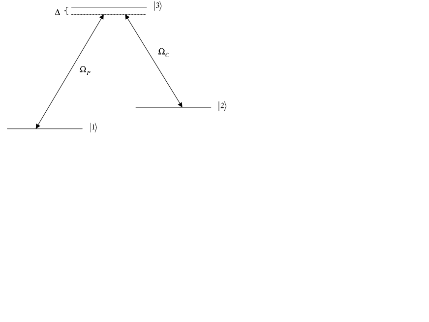
Figure 1: Level diagram for EIT. A DFS can be formed from levels $|1\rangle$ and $|2\rangle$.

The effective system Hamiltonian is found by (a) transforming to the interaction picture, (b) imposing the rotating-wave approximation, (c) a further transformation to remove the remaining explicit time dependence from the Hamiltonian. In this rotating-wave picture Shore:book ; Berman:94 the result in the ordered basis $\{\left|{i}\right\rangle\}_{i=1}^{N+1}$ is:

$$\mathbf{H}_{S} = \left(\begin{array}[]{ccccc}\Delta+\delta_{1}&0&\cdots&0&-{{{\rm\Omega}}_{1}/2}\\ 0&\Delta+\delta_{2}&&&-{{{\rm\Omega}}_{2}/2}\\ \vdots&&\ddots&&\vdots\\ 0&&&\Delta&-{{{\rm\Omega}}_{N}/2}\\ -{{{\rm\Omega}}_{1}/2}&-{{{\rm\Omega}}_{2}/2}&\cdots&-{{{\rm\Omega}}_{N}/2}&0\end{array}\right)$$ (28)

$$= \sum_{i=1}^{N}(\Delta+\delta_{i})\mathbf{T}_{ii}-\frac{1}{2}\sum_{i=1}^{N}{\rm\Omega}_{i}\mathbf{T}_{i,N+1}+{{{\rm\Omega}}_{i}}\mathbf{T}_{N+1,i}$$ (29)

where the transition operators $\{\mathbf{T}_{ab}\}$ are defined by

$$\mathbf{T}_{ab}=\left|{a}\right\rangle\left\langle{b}\right|,\quad(a,b\in\left\{{1,...,N+1}\right\}),$$

${\rm\Omega}_{i}$ is the Rabi frequency of a laser field coupling levels $|i\rangle$ and $|N+1\rangle$, $\Delta={\rm\Omega}_{i}-\omega_{N+1,i}$ is the coupling laser detuning (assumed independent of $i$), and $\delta_{i}={\rm\Omega}_{i+1}-{\rm\Omega}_{i}-\omega_{i+1,i}$ is the Raman detuning. In standard EIT ${{{\rm\Omega}}_{1}={\rm\Omega}}_{P}$ and ${{\rm\Omega}}_{2}={{\rm\Omega}}_{C}$.

Decoherence is described in this model by spontaneous emission from the excited state $|N+1\rangle$ to any of the lower lying states $|i\rangle$, where $i=1..N$. It is this decoherence process that we wish to avoid. Thus the relevant Lindblad operators $\{\mathbf{F}_{\alpha}\}$ are $\{\mathbf{T}_{i,N+1}\}$ and the $a_{\alpha\beta}$ matrix of Eq. (8) is diagonal: $a_{ii}=A_{N+1,i}$, where $A_{N+1,i}$ is the Einstein $A$ -coefficient for the spontaneous transition from $|N+1\rangle$ to $|i\rangle$. The DFS condition, Eq. (16), now tells us that if ${\left|{\psi}\right\rangle\in}\tilde{\mathcal{H}}$, then

$$\mathbf{T}_{i,N+1}{\left|{\psi}\right\rangle=c}_{i}{\left|{\psi}\right\rangle.}$$ (30)

However, note that while the operators $\{\mathbf{T}_{ij}\}$ ($i,j=1..N+1$) generate the full semisimple Lie algebra $su\left({N+1}\right)$, the $N$ operators $\{\mathbf{T}_{i,N+1}\}$ appearing in the decoherence term of the Lindblad equation, commute. They span the Abelian Cartan subalgebra [generally $su\left({N+1}\right)$ has an $N$-dimensional Cartan subalgebra, defined as the maximal set of commuting generators] Cornwell:97 . This algebra is not semisimple (since it is an Abelian invariant subalgebra of itself) and the DFS theorem does not tell us what the $\{{c}_{i}\}$ are. However, a direct way to see this is to calculate the scalar product of (30) with itself ($i\neq j$ ):

$$c_{j}^{\ast}c_{i}=\langle\psi|\mathbf{T}_{j,N+1}^{\dagger}\mathbf{T}_{i,N+1}{\left|{\psi}\right\rangle=}\langle\psi|N+1\rangle\langle j|i\rangle\langle N+1|\psi\rangle=0,$$ (31)

so that either $c_{i}=0$, or $c_{j}=0$, or both. Suppose $c_{j}=0$; then by Eq. (30) the most general form $|\psi\rangle$ can have is:

$$|\psi\rangle=\sum_{j=1}^{N}a_{j}|j\rangle,$$ (32)

i.e., $|\psi\rangle$ cannot have a component $|N+1\rangle$: $\langle N+1|\psi\rangle=0$. Thus $c_{i}=0$ for all $i$. This result for the allowed DFS states is intuitively obvious: since spontaneous emission takes place only from level $N+1$, the DF states are those which do not contain an $|N+1\rangle$ component.

Let us now take into account the requirement that the DFS be invariant under the system Hamiltonian. Invariance implies $\mathbf{T}_{k,N+1}(\mathbf{H}_{S}|\psi\rangle)=0$, so that by Eq. (30), a necessary condition is

$$[\mathbf{T}_{k,N+1},\mathbf{H}_{S}]|\psi\rangle=0.$$ (33)

Noting that $[\mathbf{T}_{k,N+1},\mathbf{T}_{ij}]=\delta_{i,N+1}|k\rangle\langle j|-\delta_{jk}|i\rangle\langle N+1|$, we can evaluate the commutator in Eq. (33) as follows:

$$[\mathbf{T}_{k,N+1},\mathbf{H}_{S}] = \sum_{i=1}^{N}(\Delta+\delta_{i})[\mathbf{T}_{k,N+1},\mathbf{T}_{ii}]$$

$$- \frac{1}{2}\sum_{i=1}^{N}{\rm\Omega}_{i}[\mathbf{T}_{k,N+1},\mathbf{T}_{i,N+1}]+{{{\rm\Omega}}_{i}[}\mathbf{T}_{k,N+1},\mathbf{T}_{N+1,i}]$$

$$= -\sum_{i=1}^{N}(\Delta+\delta_{i})\delta_{ik}|i\rangle\langle N+1|$$

$$+ \frac{1}{2}\sum_{i=1}^{N}{\rm\Omega}_{i}\delta_{N+1,k}|i\rangle\langle N+1|+{{{\rm\Omega}}_{i}}\left(\delta_{ik}|N+1\rangle\langle N+1|-|k\rangle\langle i|\right).$$

Using $\langle N+1|\psi\rangle=0$, we obtain:

$$[\mathbf{T}_{k,N+1},\mathbf{H}_{S}]|\psi\rangle=-\frac{1}{2}\left[\sum_{i=1}^{N}{{{\rm\Omega}}_{i}}\langle i|\psi\rangle\right]|k\rangle=0.$$ (34)

This leads to a generalized EIT condition:

$$\sum_{i=1}^{N}{{{\rm\Omega}}_{i}}\langle\psi|i\rangle=0,$$ (35)

which expresses a destructive interference between all $N$ lower lying levels. The corresponding superposition suffers no spontaneous emission, and is preserved under its system Hamiltonian. The standard EIT condition, for $N=2$, is

$${{\rm\Omega}}_{P}\langle{\psi}\left|{1}\right\rangle+{{\rm\Omega}}_{C}\langle{\psi}\left|{2}\right\rangle=0$$ (36)

also known as the dark-state-condition Harris:97 .

The $N-2$ dimensional DFS defined by Eqs. (32),(35) may be useful for quantum memory applications. However, it is not clear how to make use of this DFS for quantum computing applications, since all states in this DFS are degenerate eigenvectors of $\mathbf{H}_{S}$, so that the evolution inside the DFS is trivial, i.e., a global phase. This further implies that the Raman detunings $\delta_{j}$ must all vanish in order for the DFS to be preserved under $\mathbf{H}_{S}$. Finally, the symmetry that characterizes this EIT-DFS is the coupling of all spontaneous emission operators to a common excited state. A DFS would not exist if all levels were radiatively coupled to each other.

6.2 Spin Boson Model with Strong Collective Decoherence

A beautiful example of a DFS with applications to quantum computing comes from the spin-boson model Leggett:87 . This DFS example was proposed by Zanardi and Rasetti in the influential paper Zanardi:97c . Consider $N$ spins interacting with a bosonic field via the Hamiltonian

$$\mathbf{H}_{I}=\sum_{i=1}^{N}\sum_{k}\left(g_{i,k}^{+}\sigma_{i}^{+}\otimes b_{k}+g_{i,k}^{-}\sigma_{i}^{-}\otimes b_{k}^{\dagger}+g_{i,k}^{z}\sigma_{i}^{z}\otimes(b_{k}+b_{k}^{\dagger})\right).$$ (37)

Here $\{\sigma_{i}^{+},\sigma_{i}^{-},\sigma_{i}^{z}\}$ are Pauli operators acting on the $i^{\mathrm{th}}$ spin, $b_{k}$ ($b_{k}^{\dagger}$) is an annihilation (creation) operator for the $k^{\mathrm{th}}$ bosonic mode, and $g_{i,k}^{\alpha}$ are coupling constants. The Hamiltonian $\mathbf{H}_{I}$ describes a rather general interaction between a system of qubits (the spins) and a bath of bosons, exchanging energy through the $\sigma_{i}^{+}\otimes b_{k}$ and $\sigma_{i}^{-}\otimes b_{k}^{\dagger}$ terms, and changing phase through the $\sigma_{i}^{z}\otimes(b_{k}+b_{k}^{\dagger})$ term. As it stands $\mathbf{H}_{I}$ does not support a DFS: there are $3N$ $\mathbf{S}_{\alpha}$ operators  when comparing to Eq. (4), i.e., the $N$ triples of local $sl(2)$ algebras $\{\sigma_{i}^{+},\sigma_{i}^{-},\sigma_{i}^{z}\}$; each such algebra acts on a single qubit, and therefore has a two-dimensional irrep. The overall action of the total Lie algebra $\bigoplus_{i=1}^{N}sl_{i}(2)$ is represented by the irreducible $N$-fold tensor product of all local two-dimensional irreps. This implies that there are no one-dimensional irreps as required by Eq. (9), and hence no DFS.

The situation changes dramatically when a permutation symmetry is imposed on the system-bath interaction, in the form

$$g_{i,k}^{\alpha}\equiv g_{k}^{\alpha}.$$ (38)

This “collective decoherence” situation is relevant in a number of solid-state quantum computing proposals, in particular those where decoherence due to interaction with a cold phonon bath is dominant. At low temperatures only long-wavelength phonons survive (since there is an energy gap for excitation of high-energy/short-wavelength phonons), and the model of collective decoherence becomes relevant provided the qubit spacing is small compared to the phonon wavelength. Another prototypical situation is the Dicke model in quantum optics Dicke:54 , discussed in more detail below.

Given the collective decoherence assumption, one can define three collective spin operators $\mathbf{S}_{\alpha}=\sum_{i=1}^{N}\sigma_{i}^{\alpha}$ so that the Hamiltonian becomes

$$\mathbf{H}_{I}=\sum_{\alpha=+,-,z}\mathbf{S}_{\alpha}\otimes\mathbf{B}_{\alpha},$$

where $\mathbf{B}_{+}=\sum_{k}g_{k}^{+}\sigma_{i}^{+}\otimes b_{k}$, $\mathbf{B}_{-}=\mathbf{B}_{+}^{\dagger}$ and $\mathbf{B}_{z}=\sum_{k}g_{i,k}^{z}\sigma_{i}^{z}\otimes(b_{k}+b_{k}^{\dagger})$. In fact the specific form of the bath operators $\mathbf{B}_{\alpha}$ is irrelevant. The important point is that the system operators $\mathbf{S}_{\alpha}$ now form a global $sl(2)$ angular momentum algebra, i.e., $[\mathbf{S}_{+},\mathbf{S}_{-}]=\mathbf{S}_{z}$ and $[\mathbf{S}_{z},\mathbf{S}_{\pm}]=2\mathbf{S}_{\pm}$, with a highly reducible $2^{N}\times 2^{N}$ representation formed by its action on all $N$ qubits at once. We refer to the case of a global $sl(2)$ algebra as “strong collective decoherence”; the case of collective phase damping discussed in Section 3 corresponds to having just a single global angular momentum operator ($\mathbf{S}_{z}$) and is referred to as “weak collective decoherence” Kempe:00 . Since $sl(2)$ is semisimple Eq. (9) now tells us that the DFS is made up of those states $|\psi\rangle$ satisfying

$$\mathbf{S}_{\alpha}|\psi\rangle=0\qquad\forall\alpha.$$

These are the states with vanishing total (fictitious) angular momentum $J$, i.e., the “singlets” of $sl(2)$. Their explicit form is well known for the case $N=2$, in which case there is only one singlet:

$$|\psi\rangle_{N=2}\equiv|s\rangle_{12}=\frac{1}{\sqrt{2}}\left(|01\rangle-|10\rangle\right)=|J=0,m_{J}=0\rangle$$

where the notation $|s\rangle_{12}$ should be read as “singlet state of qubits 1 and 2”. This is also known as a Bell state or EPR pair Nielsen:book . The final form uses the total angular momentum $J$ and its projection $m_{J}$. It is easy to check that the state

$$|\psi\rangle_{N}=\bigotimes_{m=1}^{N/2}|s\rangle_{2m-1,2m}$$

is in the $N$-qubit DFS (since adding pairwise $|J=0,m_{J}=0\rangle$ states again produced a state with total $J=0$), and that there are no DFS states for $N$ odd (since such a state always has half-integer total $J$). The method of Young tableaux can be used to derive a dimensionality formula Zanardi:97c ; Lidar:PRA00Exchange :

$$\dim[\mathrm{DFS}(N)]=\frac{N!}{(N/2+1)!(N/2)!}$$ (39)

is the number of singlet states for $N$ qubits. An interesting consequence is that the encoding efficiency $\epsilon$ of the DFS, defined as the number of logical qubits $\log_{2}\dim[\mathrm{DFS}(N)]$ per number of  physical qubits $N$, tends asymptotically to unity Zanardi:97c :

$$\epsilon\stackrel{{\scriptstyle N\rightarrow\infty}}{{\longrightarrow}}1-\frac{3}{2}\frac{\log_{2}N}{N}.$$

There are several methods for calculating the singlet states for arbitrary $N$, e.g., by solving the problem using linear algebra, using group representation theory, or by using angular momentum addition rules. To illustrate the latter, consider the case of $N=4$. The dimensionality formula yields $\dim[\mathrm{DFS}(4)]=2$, meaning that this DFS encodes one logical qubit. One of the states is $|0_{L}\rangle\equiv|\psi\rangle_{4}=|s\rangle_{12}\otimes|s\rangle_{34}$. The second, orthogonal, state must be a combination of the triplet states $|t_{-}\rangle\equiv|00\rangle=|J=1,m_{J}=-1\rangle$, $|t_{+}\rangle\equiv|11\rangle=|J=1,m_{J}=1\rangle$, $|t_{0}\rangle\equiv\frac{1}{\sqrt{2}}\left(|01\rangle+|10\rangle\right)=|J=1,m_{J}=0\rangle$. Indeed, the combination $|1_{L}\rangle=\frac{1}{\sqrt{3}}\left(|t_{-}\rangle_{12}\otimes|t_{+}\rangle_{34}-|t_{0}\rangle_{12}\otimes|t_{0}\rangle_{34}+|t_{+}\rangle_{12}\otimes|t_{-}\rangle_{34}\right)$ clearly has total $J=0$, and has the correct Clebsch-Gordan coefficients. In this manner one can construct total $J=0$ states for progressively higher $N$.

The encoding which we just discussed, of logical qubits into blocks of four spins each, was used to provide the first constructive procedure for universal, fault tolerant quantum computation using DFSs. As shown by Bacon et al. Bacon:99a , universality can be achieved by switching on/off only Heisenberg exchange interactions between pairs of spins. This established for the first time that the Heisenberg interaction is all by itself universal for quantum computation. This observation is very important for a class of solid-state quantum computing proposals, such as electron spins in quantum dots Loss:98 and donor atom spins in Si Kane:98 , where it is technically preferable to have to control only a single interaction. The universality of the Heisenberg interaction was further proved for encodings into any number $N\geq 3$ of spins in Kempe:00 . Explicit pulse sequences for the $N=3$ case were derived in DiVincenzo:00a . Furthermore, the collective decoherence conditions can be created from arbitrary linear system-bath interaction Hamiltonians, using strong and fast pulses of the Heisenberg interaction WuLidar:01b , and leakage from a DFS can be detected using a Heisenberg-only circuit Kempe:01 , or prevented using Heisenberg-only pulses WuByrdLidar:02 .

6.3 DFS and Dicke subradiance

A different physical situation in which DFSs arise as a consequence of a collective coupling to the environment appears in the context of the Jaynes-Cummings Hamiltonian for $N$ identical two-level atoms coupled to a single mode radiation field. The Hamiltonian is very similar to that of Eq. (37), namely

$$\mathbf{H}_{I}=\sum_{i=1}^{N}\left(g_{i}^{+}\sigma_{i}^{+}\otimes b+g_{i}^{-}\sigma_{i}^{-}\otimes b^{\dagger}\right)$$ (40)

When the atoms are closer together than the wavelength of the radiation field, then the coupling parameter $g_{i}$ becomes independent of the atom index $i$, and one can write Eq. (40) in terms of the collective spin operators $\mathbf{S}_{+}=\sum_{i=1}^{N}\sigma_{i}^{+}$ and $\mathbf{S}_{-}=\sum_{i=1}^{N}\sigma_{i}^{-}$. The DFS condition may be applied directly in the Hamiltonian formulation. Together, these two conditions on the $N$-particle atomic states are equivalent to the single condition $\mathbf{S}|\psi\rangle=0$ that we derived above for the collective decoherence of the spin-boson model in the strong coupling situation (i.e., $\alpha=1,2,$ and $3$). With the atomic states alone, we therefore similarly arrive at a set of DF states that are identified with the $N$-atom singlet states. This model was also treated extensively in Duan:98b ; Duan:98c ; Zanardi:98a ; Zanardi:97b .

The Jaynes-Cummings Hamiltonian is important also in the context of the Dicke states of quantum optics Dicke:54 , where the motivation is very different from ours. The Dicke states are collective atomic states that are useful in consideration of the treatment of radiation by a collection of $N$ two-level atoms. Let $m\equiv\frac{1}{2}[($number of atoms in the excited state$)-($number in the ground state$)]$. The Dicke states are defined as eigenstates of the collective angular momentum, itself defined by $\mathbf{S}^{2}=\mathbf{S}_{x}^{2}+\mathbf{S}_{y}^{2}+\mathbf{S}_{z}^{2}$, with eigenvalues $|m|\leq J\leq N/2$, where the effective total angular momentum $J$ is referred to by Dicke as the “cooperation number” Dicke:54 ; Mandel:95 . Dicke showed that the rate of photon emission is given by $\Gamma=A(J+m)(J-m+1)$, where $A$ is the single-atom Einstein coefficient. Dicke’s interest was primarily in the “superradiant” states with $J=N/2$ and $m=0$. In this case the rate of emission is proportional to $N^{2}$, which is unusual since it implies that the radiation from a partially excited atomic system ($m=0$) can be much higher than that from a fully excited system ($m=N/2$). It also follows that there are “anti-superradiant”, or “subradiant” states, with $\Gamma=0$, corresponding to the situations $m=-J$ and $J=m=0$ Dicke:54 ; Mandel:95 . Evidence of this behavior has been obtained experimentally for trapped ions DeVoe:96 . The case $J=m=0$ coincides with that of a DFS spanned by singlet states. However, one should not conclude that DFSs are nothing but Dicke’s subradiant states. First of all, there is a major conceptual difference, since in DFS theory we consider the radiation field as an external environment, while in Dicke’s analysis the notion of an environment did not play a central role. In fact the explanation of subradiance is straightforward: the atomic dipoles are oppositely phased in pairs, so that the field radiated by one atom is absorbed by another Mandel:95 . This effect was already observed in 1970 with atoms close to a metallic mirror Drexhage:70 : the mirror image of one atom behaves as a second radiator in antiphase with the first. Secondly, the DFS conditions given in Section 5 are far more general than the Dicke states. This will become even more apparent in our discussion on DF subsystems, in Section 7. Within the formal analysis provided by the DFS conditions the Dicke states appear naturally as those states that are isolated against any interactions with the radiation field.

To further emphasize the distinction between Dicke states and DFS theory, we consider an interesting extension of these collective atomic states, that results when one incorporates the single field mode into the system, and distinguishes this from an external environment of other radiation modes. This is the situation relevant to a set of $N$ atoms interacting with a single mode in a high-finesse optical cavity, where this single cavity mode couples to a free radiation field: the prototypical situation in cavity-QED Berman:94 . The Hamiltonian is now

$$\mathbf{H}=\sum_{i=1}^{N}\left(g_{i}^{+}\sigma_{i}^{+}\otimes b+g_{i}^{-}\sigma_{i}^{-}\otimes b^{\dagger}\right)+\sum_{\lambda}\left(s_{\lambda}^{-}a_{\lambda}b^{\dagger}+s_{\lambda}^{+}a_{\lambda}^{\dagger}b\right)$$ (41)

and the system-environment interaction consists only of the second sum, since the atom-cavity mode interaction is now within the expanded system of atom plus cavity mode. In this case we find a single DFS condition, $b|\psi\rangle|n\rangle\propto|\psi\rangle|n\rangle$ where $|\psi\rangle$ is the collective atomic state $|n\rangle$ is the cavity number state. This condition implies that $b|n\rangle=0$, i.e., the cavity mode must be empty, but does not otherwise place any restrictions on the atomic component of the system state. It is only when one imposes a further requirement that the system Hamiltonian not cause system states to evolve outside the DFS that one arrives at specific atomic states. In particular, this requirement tells us that both $\mathbf{S}_{+}b$ and $\mathbf{S}_{-}b^{\dagger}$ act on $|\psi\rangle|0\rangle$ to produce at most another state $|\psi^{\prime}\rangle|0\rangle$. Since $b|0\rangle=0$, the first condition is trivially satisfied, while the second condition reduces to $\mathbf{S}_{-}|\psi\rangle=0$ because $b^{\dagger}|0\rangle=|1\rangle$ which would take the joint state outside the DFS. Thus the requirement for a DFS of the coupled $N$ atom/cavity system is simply $\mathbf{S}_{-}|\psi\rangle=0$, with a zero cavity occupation number. The atomic component of this DFS state is equal to the lowest Dicke state $|J,-J\rangle$, which constitute the ground state for a given cooperation number $J$ Mandel:95 . For $N=2$ we find a two-dimensional DFS given by the atomic states $|J=1,m=-1\rangle=|00\rangle$ and $|J=0,m=0\rangle=(1/\sqrt{2})[|10\rangle-|01\rangle]$ (combined of course with the zero cavity mode state $|n=0\rangle$). The corresponding DFS for higher values of $N$ may be readily generated using angular momentum algebra, as described in Mandel:95 . The dimensionality of these atom/cavity DFS differ from that of collective decoherence given above [Eq. (39)], being given by the expression

$$\dim[\mathrm{DFS}(N_{J})]=\frac{(2J+1)N!}{(N/2+J+1)!(N/2-J)!}$$ (42)

which reduces to Eq. (39) when $J=0$. Proposals for employing qubits encoded into these atom/cavity DFSs have been made recently by Beige et al., including discussion of performing quantum computation on the states using the quantum Zeno effect Beige:99 ; Beige:00 .

6.4 Multiple Qubit Errors

The collective decoherence example assumes that all qubits couple to the bath in a symmetric manner, which is the consequence of full permutational symmetry. However, the symmetry that gives rise to a DFS can be less strict. Consider the case of $N=4$ qubits which can undergo bit flips $\sigma_{j}^{x}$: $|0\rangle_{j}\longleftrightarrow|1\rangle_{j}$. Suppose that the qubits are arranged in pairs, such that the bit flip error affects at least two at a time. Specifically, let the allowed errors be $Q_{X}(4)=\{I,\sigma_{1}^{x}\sigma_{2}^{x},\sigma_{3}^{x}\sigma_{4}^{x},\sigma_{1}^{x}\sigma_{2}^{x}\sigma_{3}^{x}\sigma_{4}^{x}\}$, where $I$ is the identity operator (no error). Note that the error $\sigma_{2}^{x}\sigma_{3}^{x}$ is assumed not to happen. A general error in this model is a Kraus operator formed by an arbitrary linear combination of the elements of (the Abelian group) $Q_{X}(4)$. It is then simple to verify that the encoding

$$|0_{L}0_{L}\rangle = \frac{1}{2}\left(|0000\rangle+|1100\rangle+|0011\rangle+|1111\rangle\right)$$

$$|0_{L}1_{L}\rangle = \frac{1}{2}\left(|0001\rangle+|1101\rangle+|0010\rangle+|1110\rangle\right)$$

$$|1_{L}0_{L}\rangle = \frac{1}{2}\left(|0100\rangle+|1000\rangle+|0111\rangle+|1011\rangle\right)$$

$$|1_{L}1_{L}\rangle = \frac{1}{2}\left(|1001\rangle+|0101\rangle+|1010\rangle+|0110\rangle\right)$$

is a 4-dimensional DFS (denoted $DFS_{Q_{X}(4)}$), thus encoding two logical qubits. To see this, check that all states in $DFS_{Q_{X}(4)}$ are eigenstates with the same eigenvalue $+1$ of any linear combination of operators over $Q_{X}(4)$. This means that the action of the errors in $Q_{X}(4)$ is to leave the subspace $DFS_{Q_{X}(4)}$ invariant, so that this subspace is DF, in accordance with Theorem 5.3 and the more general Theorem 5.2. The latter theorem, however, only requires that the Kraus operators have an identical unitary representation on the DFS, which means that eigenvalues other than $+1$ are possible in principle. Indeed, it is simple to check that the state $(|0000\rangle-|1100\rangle+|0011\rangle-|1111\rangle)/2$ belongs to another $4$ -dimensional DFS, characterized by the eigenvalue $-1$. In fact the entire $16$-dimensional Hilbert space splits up into four $4$-dimensional DFSs, two with eigenvalue $+1$, two with eigenvalue $-1$.

In order to generalize this result, note that the group $Q_{X}(4)$ is generated (under multiplication) by $\sigma_{1}^{x}\sigma_{2}^{x}$ and $\sigma_{3}^{x}\sigma_{4}^{x}$; clearly the group $Q_{X}(N)$ generated by $\{\sigma_{2j-1}^{x}\sigma_{2j}^{x}\}_{j=1}^{N/2}$ also supports a DFS with the same defining property, namely that the DF states are simultaneous eigenstates of all $Q_{X}(N)$ generators.

Even more generally, the type of DFS considered here is an example of a DFS for multiple qubit errors. The general theory is worked out in Lidar:00a . The error model can be stated abstractly as follows: Starting from the Pauli group on $N$ qubits (the group of $N$-fold tensor products of the Pauli matrices $\{\sigma_{x},\sigma_{y},\sigma_{z}\}$), look for Abelian subgroups. Every such subgroup defines an error model, in the sense that linear combinations of elements of the subgroup form Kraus operators. The physical motivation for such subgroups is: (i) The case in which either only higher order (multiple qubit) errors occur, such that first-order terms of the form $I\otimes\cdots\otimes I\otimes\sigma_{i}^{\alpha}\otimes I\otimes\cdots\otimes I$ are absent in the Pauli-group expansion of the Kraus operators, or (ii) only errors of one kind, either $\sigma^{x}$, $\sigma^{y}$, or $\sigma^{z}$ take place. Case (i) would imply that there are certain cancellations involving bath matrix element terms such that first-order system operators are absent in the expansion of Eq. (6). While this would be a rather non-generic situation, involving a very special “friendly” bath, it turns out that such conditions can be actively generated from arbitrary baths using fast and strong, dynamical decoupling pulses WuLidar:01b . Alternatively, in case (i) the system-bath Hamiltonian does not have the general form of Eq. (4), but rather involves only second order terms such as $\sigma_{i}^{\alpha}\otimes\sigma_{j}^{\beta}$ (identity on all the rest). Case (ii) is applicable in, e.g., the case of pure phase damping (relevant to NMR Slichter:book ) and optical lattices using cold controlled collisions Jaksch:99 ), where $\sigma^{z}$ errors are dominant. When either condition (i) or (ii) above is satisfied, the subgroup is Abelian, which is a necessary condition for it to have one-dimensional irreps. This, in turn, is a necessary and sufficient condition for a DFS by Theorem 5.2. Thus, to every such multiple qubit error model there corresponds a DFS, which is found by studying the one-dimensional irreps of the subgroup over $N$ qubits. The DFS basis states are states that transform according to a one-dimensional irrep with fixed eigenvalue. The dimension of such a DFS therefore turns out to be the multiplicity of the one-dimensional irreps of the subgroup. The result seen above for $Q_{X}(4)$ is general: the entire Hilbert space splits up into equi-dimensional, independent DFSs Lidar:00a . It is also possible to perform universal, fault tolerant quantum computation on these DFSs, by using a hybrid DFS-QECC method Lidar:00b . An experimental magnetic resonance realization of DF quantum computation, implementing Grover’s algorithm in the presence of multiple-qubit errors, has recently been completed Ollerenshaw:02 .

7 Decoherence-Free (Noiseless) Subsystems

As long as we restrict our attention to encoding quantum information in a DF manner over a subspace then Eqs. (9),(16) provide necessary and sufficient conditions for the existence of such DFSs. The notion of a subspace which remains DF throughout the evolution of a system is not, however, the most general method for providing DF encoding of information in a quantum system. Knill, Laflamme, and Viola Knill:99a discovered a method for DF encoding into subsystems instead of into subspaces. Zanardi soon thereafter realized that this opened the door to a unification of many of the previously seemingly unrelated ideas for reducing decoherence Zanardi:99d . Related, less general results were independently derived in DeFilippo:00 ; Yang:01 . Kempe et al. developed a general theory of universal quantum computation based on the DF subsystems concept Kempe:00 .

7.1 Formal Theory

We first introduce a formal characterization of DF subsystems. This is most easily done in the Hamiltonian formulation of decoherence. Let $\mathcal{A}$ denote the associative algebra (i.e., the algebra of all polynomials) generated by the system Hamiltonian $\mathbf{H}_{S}$ and the system components of the interaction Hamiltonian, the $\mathbf{S}_{\alpha}$’s of Eq. (4). We assume that $\mathbf{H}_{S}$ is expressed in terms of the $\mathbf{S}_{\alpha}$’s as well (if needed we can always enlarge this set), and that the identity operator is included as $\mathbf{S}_{0}=\mathbf{I}_{S}$ and $\mathbf{B}_{0}=\mathbf{I}_{B}$. This will have no observable consequence but allows for the use of an important representation theorem. Because the Hamiltonian is Hermitian the $\mathbf{S}_{\alpha}$’s must be closed under Hermitian conjugation: $\mathcal{A}$ is a “$\dagger$-closed” operator algebra. A basic theorem of such operator algebras which include the identity operator states that, in general, $\mathcal{A}$ will be a reducible subalgebra of the full algebra of operators on the system Hilbert space $\mathcal{H}_{S}$ Landsman:98a . This means that the algebra is isomorphic to a direct sum of $d_{J}\times d_{J}$ complex matrix algebras $\mathcal{M}(d_{J})$, each with multiplicity $n_{J}$:

$$\mathcal{A}\cong\bigoplus_{J\in\mathcal{J}}\mathbf{I}_{n_{J}}\otimes\mathcal{M}(d_{J}).$$ (43)

Here $\mathcal{J}$ is a finite set labeling the irreducible components of $\mathcal{A}$.

The structure implied by Eq. (43) is illustrated schematically as follows, for some system operator $\mathbf{S}_{\alpha}$:

⋱J=|𝒥|]subscript𝐒𝛼delimited-[]fragments fragments missing-subexpressionmissing-subexpression⋱missing-subexpressionmissing-subexpressionmissing-subexpressionmissing-subexpressionfragmentsJ|J|\mathbf{S}_{\alpha}=\left[\begin{tabular}[]{cccc}\cline{1-1}\cr\vrule\lx@intercol\hfil$J=1$\hfil\lx@intercol &\vrule\lx@intercol\hfil\hfil\lx@intercol &&\\ \cline{1-2}\cr&\vrule\lx@intercol\hfil$J=2$\hfil\lx@intercol &\vrule\lx@intercol\hfil\hfil\lx@intercol &\\ \cline{2-2}\cr&&$\ddots$&\\ \cline{4-4}\cr&&&\vrule\lx@intercol\hfil$J=|\mathcal{J}|$\hfil\lx@intercol\vrule\lx@intercol \\ \cline{4-4}\cr\end{tabular}\ \right]

=J1=J2=J1=J2 (44)

In this block diagonal matrix representation, a typical block with given $J$, may have a further block diagonal structure,

$$\left[\begin{tabular}[]{cccccccccc}\cline{1-3}\cr\vrule\lx@intercol\hfil\hfil\lx@intercol &&&\vrule\lx@intercol\hfil\hfil\lx@intercol &&&&&&\\ \vrule\lx@intercol\hfil\hfil\lx@intercol &$M_{\alpha}$&&\vrule\lx@intercol\hfil\hfil\lx@intercol &&&&&&\\ \vrule\lx@intercol\hfil\hfil\lx@intercol &&&\vrule\lx@intercol\hfil\hfil\lx@intercol &&&$\mu$&&&\\ \cline{1-6}\cr&&&\vrule\lx@intercol\hfil\hfil\lx@intercol &&&\vrule\lx@intercol\hfil$0$\hfil\lx@intercol &&&\\ &&&\vrule\lx@intercol\hfil\hfil\lx@intercol &$M_{\alpha}$&&\vrule\lx@intercol\hfil$\vdots$\hfil\lx@intercol &&&\\ &&&\vrule\lx@intercol\hfil\hfil\lx@intercol &&&\vrule\lx@intercol\hfil$d_{J}-1$\hfil\lx@intercol &&&\\ \cline{4-6}\cr&&$\mu^{\prime}:$&$0$&$\cdots$&$d_{J}-1$&$\ddots$&&&\\ \cline{8-9}\cr&&&&&&&\vrule\lx@intercol\hfil\hfil\lx@intercol &&\vrule\lx@intercol\hfil\hfil\lx@intercol \\ &&&&&&&\vrule\lx@intercol\hfil\hfil\lx@intercol &$M_{\alpha}$&\vrule\lx@intercol\hfil\hfil\lx@intercol \\ &&&&&&&\vrule\lx@intercol\hfil\hfil\lx@intercol &&\vrule\lx@intercol\hfil\hfil\lx@intercol \\ \cline{8-9}\cr\end{tabular}\ \right]\begin{tabular}[]{c}\\ $\lambda=0$\\ \\ \\ \\ $\lambda=1$\\ \\ \\ \\ \\ \\ \end{tabular}$$ (45)

Here $\lambda$ labels the different degenerate sub-blocks, and $\mu$ labels the states inside each sub-block. Associated with this decomposition of the algebra $\mathcal{A}$ is the decomposition over the system Hilbert space:

$$\mathcal{H}_{S}=\sum_{J\in\mathcal{J}}{\rm\kern 2.40005pt\vrule width=0.39993pt,height=6.28612pt,depth=-0.3014pt\kern-3.00003ptC}^{n_{J}}\otimes{\rm\kern 2.40005pt\vrule width=0.39993pt,height=6.28612pt,depth=-0.3014pt\kern-3.00003ptC}^{d_{J}}.$$ (46)

DF subsystems are defined as the situation in which information is encoded in a single component ${\rm\kern 2.40005pt\vrule width=0.39993pt,height=6.28612pt,depth=-0.3014pt\kern-3.00003ptC}^{n_{J}}$ of Eq. (46) (thus the dimension of the DF subsystem is $n_{J}$). The decomposition in Eq. (43) reveals that information encoded in such a subsystem will always be affected as identity on the component ${\rm\kern 2.40005pt\vrule width=0.39993pt,height=6.28612pt,depth=-0.3014pt\kern-3.00003ptC}^{n_{J}}$, and thus this information will not decohere. This deep fact is the basis for the theory of DF subsystems.

Several general observations are in order: (i) The tensor product structure which gives rise to the name subsystem in Eq. (43) is a tensor product over a direct sum, and therefore will not in general correspond to the natural tensor product of (spatially distinguishable) qubits; (ii) The subsystem nature of the decoherence implies that the information should be encoded in a separable way: over the tensor structure of Eq. (46) the density matrix should split into two valid density matrices: $\mathbf{\rho}_{S}(0)=\mathbf{\rho}\otimes\mathbf{\gamma}$ where $\mathbf{\rho}$ is the DF subsystem and $\mathbf{\gamma}$ is the corresponding component of the density matrix which does decohere; (iii) Not all of the subsystems in the different irreducible representations can be simultaneously used: (phase) decoherence will occur between the different irreducible components of the Hilbert space labeled by $J\in\mathcal{J}$. For this reason, from now on we restrict our attention to the subsystem defined by a given $J$.

DF subspaces are now easily connected to DF subsystems. DF subspaces correspond to those DF subsystems possessing one-dimensional irreducible matrix algebras: $\mathcal{M}(1)$. The multiplicity of these one-dimensional irreducible algebras is the dimension of the DF subspaces. In fact it is easy to see how the DF subsystems arise out of a non-commuting generalization of the DF subspace conditions. Let $\{|\lambda_{\mu}\rangle\}$, $1\leq\lambda\leq n_{J}$ and $1\leq\mu\leq d_{J}$, denote a subsystem of $\mathcal{H}_{S}$ with given $J$. Then the condition for the existence of an irreducible decomposition as in Eq. (43) is

$$\mathbf{S}_{\alpha}|\lambda_{\mu}\rangle=\sum_{\mu^{\prime}=1}^{d_{J}}M_{\mu\mu^{\prime},\alpha}|\lambda_{\mu^{\prime}}\rangle,$$ (47)

for all $\mathbf{S}_{\alpha}$, $\lambda$ and $\mu$. Note that $M_{\mu\mu^{\prime},\alpha}$ is not dependent on $\lambda$, in the same way that $c_{\alpha}$ in Eq. (9) is the same for all states $|\tilde{k}\rangle$ (there $\mu=1$ and fixed). Thus for a fixed $\lambda$, the subsystem spanned by $|\lambda_{\mu}\rangle$ is acted upon in some nontrivial way. However, because $M_{\mu\mu^{\prime},\alpha}$ is not dependent on $\lambda$, each subsystem defined by a fixed $\mu$ and running over $\lambda$ is acted upon in an identical manner by the decoherence process.

The generalization of the Lindblad semigroup formulation of the DF subspace condition to the corresponding master equation for a DF subsystem is not trivial. This is because the $\mathbf{F}_{\alpha}$ operators in Eq. (8) are not required to be closed under conjugation. The representation theorem Eq. (43) is hence not directly applicable. It can be shown, however, that the master equation analog of Eq. (47) is:$\ \mathbf{F}_{\alpha}|\lambda_{\mu}\rangle=\sum_{\mu^{\prime}=1}^{d_{J}}M_{\mu\mu^{\prime},\alpha}|\lambda_{\mu^{\prime}}\rangle$, and provides a necessary and sufficient condition for the preservation of DF subsystems. For details the reader is referred to (Kempe:00, , p.5).

As noted before, the subsystems concept is crucial in establishing a general theory of universal, fault tolerant quantum computation over DFSs. To this end it is necessary to introduce the commutant $\mathcal{A}^{\prime}$ of $\mathcal{A}$. This is the set of operators which commutes with the algebra $\mathcal{A}$, $\mathcal{A}^{\prime}=\left\{\mathbf{X}:[\mathbf{X},\mathbf{A}]=0,\forall\mathbf{A}\in\mathcal{A}\right\}$. They also form a $\dagger$-closed algebra, which is reducible to

$$\mathcal{A}^{\prime}=\bigoplus_{J\in\mathcal{J}}\mathcal{M}(n_{J})\otimes\mathbf{I}_{d_{J}}$$ (48)

over the same basis as $\mathcal{A}$ in Eq. (43). Comparing to Eq. (43) it is clear that non-trivial operators in $\mathcal{A}^{\prime}$ are exactly the transformations that preserve the DFS Zanardi:99a . As shown in detail in Kempe:00 , this allows for a constructive proof that the Heisenberg exchange interaction is universal over all DFS encodings for collective decoherence.

7.2 Examples

To illustrate the DF states that emerge from the subsystems formulation it is convenient to use once more the collective decoherence model. As will be recalled from Section 6.2, “strong” collective decoherence on $N$ qubits is characterized by the three system operators $\mathbf{S}_{+}$, $\mathbf{S}_{-}$ and $\mathbf{S}_{z}$. These operators form a representation of the semisimple Lie algebra $sl(2)$. The algebra $\mathcal{A}$ generated by these operators can be decomposed as

$$\mathcal{A}\cong\bigoplus_{J=0(1/2)}^{N/2}\mathbf{I}_{n_{J}}\otimes gl(2J+1)$$ (49)

where $J$ labels the total angular momentum of the corresponding Hilbert space decomposition (and hence the $0$ or $1/2$ depending on whether $N$ is even or odd respectively) and $gl(2J+1)$ is the general linear algebra acting on a space of size $2J+1$. The resulting decomposition of the system Hilbert space

$$\mathcal{H}_{S}\cong\bigoplus_{J=0(1/2)}^{N/2}{\rm\kern 2.40005pt\vrule width=0.39993pt,height=6.28612pt,depth=-0.3014pt\kern-3.00003ptC}_{n_{J}}\otimes{\rm\kern 2.40005pt\vrule width=0.39993pt,height=6.28612pt,depth=-0.3014pt\kern-3.00003ptC}_{2J+1}$$ (50)

is exactly the reduction of the Hilbert states into different Dicke states Dicke:54 ; Mandel:95 . The degeneracy for each $J$ is therefore given by Eq. (42). Eq. (49) shows that given $J$, a state $|J,\lambda,\mu\rangle$ is acted upon as identity on its $\lambda$ component. Thus a DFS is defined by fixing $J$ and $\mu$, where $\mu$ can now be naturally interpreted as the $z$-component of the projection of the total angular momentum. As we will show shortly, $\lambda$ corresponds to the degeneracy of paths leading to a given node $(N,J)$ on the diagram of Fig. (2). In the strong collective decoherence case, we shall denote the $N$-qubit DFS labeled by a particular angular momentum $J$, by $DFS_{N}(J)$.

The DFSs corresponding to the different $J$ values for a given $N$ can be computed using standard methods for the addition of angular momentum. We use the convention that $|1\rangle$ represents a $|j=1/2,m_{j}=1/2\rangle$ particle and $|0\rangle$ represents a $|j=1/2,m_{j}=-1/2\rangle$ particle in this decomposition although, of course, one should be careful to treat this labeling as strictly symbolic and not related to the physical angular momentum of the particles.

The smallest $N$ which supports a DFS and encodes at least a qubit of information is $N=3$ Knill:99a ; DeFilippo:00 ; Yang:01 . In this case there are two possible values of the total angular momentum: $J=3/2$ or $J=1/2$. The four $J=3/2$ states $|J,\lambda,\mu\rangle=|3/2,0,\mu\rangle$ ($\mu=m_{J}=\pm 3/2,\pm 1/2$) are singly degenerate; the $J=1/2$ states have degeneracy $2$. They can be constructed by either adding a $J_{12}=1$ (triplet) or a $J_{12}=0$ (singlet) state to a $J_{3}=1/2$ state. These two possible methods of adding the angular momentum to obtain a $J=1/2$ state are exactly the degeneracy of the algebra. The four $J=1/2$ states are:

$$\begin{array}[]{l}|{\frac{1}{2}},0,{\frac{1}{2}}\rangle={\frac{1}{\sqrt{2}}}\left(|010\rangle-|100\rangle\right)\\ |{\frac{1}{2}},0,-{\frac{1}{2}}\rangle={\frac{1}{\sqrt{2}}}\left(|011\rangle-|101\rangle\right)\end{array}$$

$$\begin{array}[]{l}|{\frac{1}{2}},1,0\rangle={\frac{1}{\sqrt{6}}}\left(-2|001\rangle+|010\rangle+|100\rangle\right)\\ |{\frac{1}{2}},1,1\rangle={\frac{1}{\sqrt{6}}}\left(2|110\rangle-|101\rangle-|011\rangle\right)\end{array}$$

where on the left we used the $|J,\lambda,\mu\rangle$ notation and on the right the states are expanded in terms the single-particle $|j=1/2,m_{j}=\pm 1/2\rangle$ basis using Clebsch-Gordan coefficients. The DF qubit can now be written compactly as

$$|0_{L}\rangle = \alpha|1/2,0,1/2\rangle+\beta|1/2,0,-1/2\rangle$$

$$|1_{L}\rangle = \alpha|1/2,1,1/2\rangle+\beta|1/2,1,-1/2\rangle$$ (53)

where $|\alpha|^{2}+|\beta|^{2}=1$, i.e., the encoding is into the degeneracy of the two $J=1/2$ subsystems. By the the decomposition of Eqs. (49),(50) it is clear that collective errors can change the $\alpha,\beta$ coefficients, but have the same effect on the $|0_{L}\rangle,|1_{L}\rangle$ states, which is why this encoding is a DFS.

The smallest DF subspace (as opposed to subsystem) supporting a full encoded qubit comes about for $n=4$. Subspaces for the strong collective decoherence mechanism correspond to the degeneracy of the zero total angular momentum eigenstates (there are also two DF subsystems with degeneracy $1$ and $3$). As we already noted in Section 6.2 this subspace is spanned by the states:

$$|0_{L}\rangle = |0,0,0\rangle=|0,0\rangle\otimes|0,0\rangle={\frac{1}{2}}|(|01\rangle-|10\rangle)(|01\rangle-|10\rangle)$$

$$|1_{L}\rangle = |0,1,0\rangle={\frac{1}{\sqrt{3}}}(|1,1\rangle\otimes|1,-1\rangle-|1,0\rangle\otimes|1,0\rangle+|1,-1\rangle\otimes|1,1\rangle)$$ (54)

$$= {\frac{1}{\sqrt{12}}}(2|0011\rangle+2|1100\rangle-|0101\rangle-|1010\rangle-|0110\rangle-|1001\rangle).$$

The notation is the same as in Eq. (53), except that in the third equality we have used the notation $|J_{12},m_{J_{12}}\rangle\otimes|J_{34},m_{J_{34}}\rangle$ which makes it easy to see how the angular momentum is added.

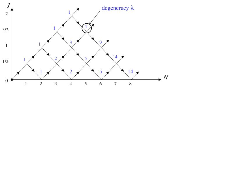
Figure 2: Partitioning of the Hilbert space of $N$ spin-$1/2$ particles into DF subspaces (nodes on the $N$-axis) and subsystems (nodes above the $N$-axis). Integer above a node represents the number of paths leading from the origin to that node, i.e., the degeneracy quantum number $\lambda$. See text for full details.

There is a simple graphical interpretation of these results, shown in Fig. (2). Starting from the origin (no spins) one starts adding spin-$1/2$ particles. The first particle ($N=1$) has total angular momentum $J=1/2$. This single particle has the trivial $DFS_{1}(1/2)$. When the second particle is added one can form either a singlet ($J=0$) by subtracting $1/2$ or form a triplet by adding $1/2$. In this manner the subspace $DFS_{2}(0)$ and subsystem $DFS_{2}(1)$ are formed, containing a single state ($\mu=m_{J}=0$) and three states ($\mu=m_{J}=-1,0,1$), respectively. The first interesting DFS is formed when $N=3$, since now there are two paths, $\lambda=0,1$, in Fig. (2) leading to the same total $J=1/2$. These two paths correspond exactly to the $|0_{L}\rangle$ and $|1_{L}\rangle$ states of Eq. (53), and define the subsystem $DFS_{3}(1/2)$, that encodes a single DF qubit. For $N=4$ spins there is the DF subspace $DFS_{4}(0)$ and also a three-dimensional DF subsystem $DFS_{4}(1)$. Clearly, the DF subspaces are simply all the nodes that lie on the $N$-axis in Fig. (2), while the DF subsystems are all the nodes above this axis. Interpreted in this manner, Fig. (2) is a partitioning of the entire system Hilbert space into disjoint DFSs. The examples presented here have been worked out in far greater detail in Kempe:00 ; Bacon:thesis ; Kempe:thesis , where it is further shown how to construct universal quantum computation operations using the same formalism.

8 Protection against additional decoherence sources

It is clear from the above summary of DF subspaces and subsystems that they will afford complete protection against the specific errors that they are designed to eliminate. However, in general it is not possible to protect agains all kinds of errors and one is motivated to then consider how to add protection of DFS encodings agains additional sources of decoherence. Several approaches have been taken to address this issue. It was shown early on that DFSs are remarkably stable to additional sources of decoherence, providing a useful point of departure for more general schemes to protect fragile quantum information. The first study to consider the effects of perturbations breaking the symmetry giving rise to a DFS was Ref. Lidar:PRL98 , within the Markovian semigroup formulation. It was shown that if an additional set of Lindblad operators are added to the Lindblad equation (8), parametrized by a coupling strength $\epsilon$, then the “mixed state fidelity” $f_{\epsilon}(t)\equiv{\rm Tr}[\rho_{\rm id}(t)\rho_{\epsilon}(t)]$, i.e., the overlap between the ideal (decoherence-free) evolution $\rho_{\rm id}(t)$ and the perturbed evolution $\rho_{\epsilon}(t)$, decays as $1-O(\epsilon t^{2})$. This conclusion was significantly strengthened in Ref. Bacon:99 , where a stability analysis was made within both the semigroup and OSR formulations. It was shown that in both formulations states in DFSs are stable to symmetry-breaking perturbations to second order in the strength of the perturbation: $f_{\epsilon}(t)=1-O(\epsilon^{2}t^{2})$, so the entire $O(\epsilon)$ contribution vanishes to all orders in time. This indicates that the DFSs are well-suited for applications to quantum memory, a result that has been recently been taken advantage of in ion traps Kielpinski:01 ; Kielpinski:02 ; Brown:02 ; LidarWu:02 . Errors that do occur can be dealt with by a number of methods: (i) Additional encoding Lidar:PRL99 ; Lidar:PRA00Exchange ; Alber:01 ; Alber:01a ; KhodjastehLidar:02 , (ii) Implementing error-detection circuits Kempe:01 ; (iii) Hamiltonian engineering to suppress or eliminate further errors Bacon:01 ; (iv) Combination with the dynamical decoupling technique WuLidar:01b ; LidarWu:02 ; WuByrdLidar:02 ; ByrdLidar:01a ; ByrdLidar:02a ; Viola:01a . We briefly summarize instances of these four approaches here.

In the collective decoherence DFS, independent single qubit errors can be shown to cause either independent errors acting on the encoded qubit states, or leakage of the DFS encoded qubit states to states lying outside the DFS Lidar:PRL99 . Both of these types of errors may be corrected by concatenating the DFS encoding with a standard quantum error-correcting code that corrects independent single qubit errors. Thus, the four qubit DFS encoding for collective decoherence was concatenated with the five-qubit QECC in Ref. Lidar:PRL99 to produce a 20-qubit encoding that provides protection against both collective and independent errors on the physical qubits. Concatenation thus provides one way to correct leakage errors that take the encoded quantum information out of the DFS.

Another approach is to implement a leakage-correction circuit Preskill:97a . An example of this for the three-qubit encoding into a subsystem protected against collective decoherence is given in Ref. Kempe:01 . Such circuits may be readily incorporated into schemes for implementing fault-tolerant computation such as in Refs. Bacon:99a ; Kempe:00 . This particular leakage-correction circuit allows correction without any measurement, providing a simpler approach than usual in protocols for fault tolerance.

The third approach to dealing with errors not specifically protected against by the DFS encoding, namely by Hamiltonian engineering to eliminate additional errors, is very different from the first two. The idea here is to supplement the qubit Hamiltonian by additional interactions that impose an energy spectrum on the DFS states. The additional Hamiltonian terms are specifically engineered to result in an energy spectrum that eliminates or thermally suppresses additional errors. This approach has been demonstrated in Ref. Bacon:01 , using the four-qubit DFS encoding against collective decoherence. Addition of a specifically designed set of exchange interactions between the physical qubits causes the qubit tensor product states in the DFS representation (Section 6.2) to split into a spectrum of higher angular momentum states that are separated from the degenerate ground state that provides the zero angular momentum DFS encoding. The effect of this additional Hamiltonian is to transform all independent single-qubit errors into non-energy conserving errors that cause excitation out of the ground state encoding. Thus all local phase errors on the encoded qubit states have been removed, while maintaining their protection against collective decoherence, leading to their designation as “coherence-preserving” or “supercoherent”. The energy-nonconserving errors can be suppressed by going to low temperatures, or alternatively, used as an error-detecting code.

The fourth approach to dealing with additional errors combines DFS encoding with the method of strong and fast dynamical decoupling pulses proposed by Viola and Lloyd in Ref. Viola:98 . The first concrete example of this approach was given by Wu and Lidar in Ref. WuLidar:01b , where it was shown that dynamical decoupling pulses can create the conditions for both the multiple-qubit and collective decoherence error models, starting from arbitrary system-bath interactions. In the latter error model, this can be done by rapidly pulsing the Heisenberg exchange interaction, so the scheme is fully compatible with universal quantum computation on the resulting DFS. However, even after the creation of the appropriate symmetry, leakage from the DFS is still possible. To this end Refs. WuByrdLidar:02 ; ByrdLidar:01a ; ByrdLidar:02a showed explicitly how leakage errors too can be eliminated using dynamical decoupling, and in the case of collective decoherence, these can again be generated using Heisenberg interactions. Integration of all these components (DFS protection, generation of symmetric system-bath interaction, and leakage elimination), has been discussed in Ref. LidarWu:02 .

These studies of effects of errors beyond the specific error models defining the DFS and its protection show that there are a number of viable approaches to incorporate DFS encodings into stronger schemes that provide protection of quantum states at multiple levels. They can be used both to further improve the performance of DFS encoded qubits for quantum memory applications, and also in implementations of quantum computation with DFS encodings Kempe:00 . Concatenation and leakage-detection circuits provide a direct route to the established framework of fault-tolerance. Similarly, the use of Hamiltonian engineering as a design tool to suppress or remove additional errors relates to the very different approach advocated by topological quantum computing, where one seeks to optimize the Hamiltonian structure to eliminate or automatically correct errors Kitaev:97 ; Kitaev:book . The DFS-dynamical decoupling combination ties in naturally with several solid state and atomic physics proposals for quantum computing. These relations deserve further exploration in the future.

9 Conclusions

This review is an introduction to the now well-developed theory of decoherence-free subspaces and subsystems (DFSs). The central idea behind DFSs is that decoherence can be avoided by encoding quantum information into special subspaces that are protected from the interaction with the environment by virtue of a dynamical symmetry. This idea has roots that can be traced to work in quantum optics, the measurement problem, and the general theory of open quantum systems. However, the appreciation of its importance to quantum information theory, the development of a rigorous underlying mathematical framework, and experimental verification, are all very recent. We have provided here a survey of these developments, emphasizing the theoretical contributions to the problem of preservation of quantum information, as opposed to the rich and fascinating subject of its manipulation. This was illustrated with examples from quantum optics and general models of interacting quantum systems. It is important to emphasize that DFSs are only one of several ideas for the preservation of quantum information, and that full protection of quantum information is likely to involve a combination at different levels of several methods. The most notable alternatives are quantum error correcting codes, geometric and topological encodings of quantum information, and dynamical suppression of decoherence via the application of fast and strong pulses. It is now increasingly apparent that there are strong unifying features to all of these ideas, in the sense that there is an underlying algebraic structure from which all the different methods seem to emerge. Future investigations will no doubt further clarify this unity, and it is our hope that new experiments will confirm the usefulness of the DFS concept, in particular for quantum information processing.

References

- (1) J. Gruska. Quantum Computing. Mc Graw-Hill, London, 1999.
- (2) A.Yu. Kitaev, A.H. Shen, M.N. Vyalyi. Classical and Quantum Computation, volume 47 of Graduate Studies in Mathematics. American Mathematical Society, Providence, RI, 2000.
- (3) M.A. Nielsen and I.L. Chuang. Quantum Computation and Quantum Information. Cambridge University Press, Cambridge, UK, 2000.
- (4) D. Giulini, E. Joos, C. Kiefer, J. Kupsch, I.-O. Stamatescu, and H.D. Zeh, editors. Decoherence and the Appearance of a Classical World in Quantum Theory. Springer-Verlag, Berlin, 1996.
- (5) R. Landauer. Is quantum mechanics useful? Proc. Roy. Soc. London Ser. A, 353:367, 1995.
- (6) W.G. Unruh. Maintaining coherence in quantum computers. Phys. Rev. A, 51:992, 1995.
- (7) The mathematical and physical relations between these two contributions to non-unitary evolution of the system have been the subject of many studies in quantum relaxation theory over the last 20 years. In the energy eigenbasis dephasing causes decay of off-diagonal elements of the density matrix, while dissipation causes decay of both diagonal and off-diagonal elements. In the context of quantum computation and error correction it has become customary to refer to both types of processes generically as ‘decoherence’. While the original meaning of decoherence was specifically designated to describe loss of coherences in the off-diagonal elements of the density operator in the energy eigenbasis, there are several reasons why one may wish to be less specific for general study of the effects of environmental interactions on quantum information processing. First, there is the undesirable fact that such decay of coherences in the off-diagonal elements of the density operator is basis set dependent. Second, at the physical level, both dissipative and dephasing interactions contribute to this loss of coherence in off-diagonal elements. These two factors render it more preferable in the context of a general consideration of quantum errors to adopt the now common usage of ‘decoherence’ to refer quite generally to loss of unitary evolution and to all underlying physical mechanisms for this.
- (8) M. Shapiro and P. Brumer. Coherent Control of Atomic, Molecular and Electronic Processes. Adv. Atomic, Mol. & Opt. Phys., 42:287, 2000.
- (9) H. Rabitz, R. de Vivie-Riedle, M. Motzkus, and Karl Kompa. Whither the Future of Controlling Quantum Phenomena? Science, 288:824, 2000.
- (10) A. Ekert and R. Jozsa. Quantum algorithms: Entanglement Enhanced Information Processing. Phil. Trans. Roy. Soc. (Lond.), 356:1769, 1998.
- (11) D. Aharonov and M. Ben-Or. Polynomial Simulations of Decohered Quantum Computers. In Proceedings of 37th Conference on Foundations of Computer Science (FOCS), page 46, Los Alamitos, CA, 1996. IEEE Comput. Soc. Press.
- (12) W.H. Zurek. Pointer basis of a quantum apparatus: Into what mixture does the wave packet collapse? Phys. Rev. D, 24:1516, 1981.
- (13) W.H. Zurek. Preferred states, predictability, classicality and the environment-induced decoherence. Prog. Theor. Phys., 89:281, 1993.
- (14) R. Alicki. Limited thermalization for the Markov mean-field model of N atoms in thermal field. Physica A, 150:455, 1988.
- (15) G.M. Palma, K.-A. Suominen and A.K. Ekert. Quantum Computers and Dissipation. Proc. Roy. Soc. London Ser. A, 452:567, 1996.
- (16) L.-M Duan and G.-C. Guo. Reducing decoherence in quantum-computer memory with all quantum bits coupling to the same environment. Phys. Rev. A, 57:737, 1998.
- (17) L.-M Duan and G.-C. Guo. Preserving Coherence in Quantum Computation by Pairing Quantum Bits. Phys. Rev. Lett., 79:1953, 1997.
- (18) P. Zanardi and M. Rasetti. Noiseless Quantum Codes. Phys. Rev. Lett., 79:3306, 1997.
- (19) P. Zanardi and M. Rasetti. Error Avoiding Quantum Codes. Mod. Phys. Lett. B, 11:1085, 1997.
- (20) P. Zanardi. Dissipative dynamics in a quantum register. Phys. Rev. A, 56:4445, 1997.
- (21) L.-M Duan and G.-C. Guo. Prevention of dissipation with two particles. Phys. Rev. A, 57:2399, 1998.
- (22) L.-M. Duan and G.-C. Guo. Optimal quantum codes for preventing collective amplitude damping. Phys. Rev. A, 58:3491, 1998.
- (23) P. Zanardi and F. Rossi. Quantum Information in Semiconductors: Noiseless Encoding in a Quantum-Dot Array. Phys. Rev. Lett., 81:4752, 1998.
- (24) P. Zanardi and F. Rossi. Subdecoherent Information Encoding in a Quantum-Dot Array. Phys. Rev. B, 59:8170, 1999.
- (25) P. Zanardi. Dissipation and decoherence in a quantum register. Phys. Rev. A, 57:3276, 1998.
- (26) D.A. Lidar, I.L. Chuang and K.B. Whaley. Decoherence free subspaces for quantum computation. Phys. Rev. Lett., 81:2594, 1998.
- (27) D.A. Lidar, D. Bacon and K.B. Whaley. Concatenating Decoherence Free Subspaces with Quantum Error Correcting Codes. Phys. Rev. Lett., 82:4556, 1999.
- (28) D.A. Lidar, D. Bacon, J. Kempe, and K.B. Whaley. Decoherence-free subspaces for multiple-qubit errors: (i) characterization. Phys. Rev. A, 63:022306, 2001.
- (29) M. Durdevich, H.E. Makaruk, R.Owczarek. Generalized Noiseless Quantum Codes utilizing Quantum Enveloping Algebras.
- (30) B. Qiao, H.E. Ruda, and M.S. Zhan. Two-qubit quantum computing in a projected subspace. Phys. Rev. A, 65:042325, 2002.
- (31) M. Shapiro and P. Brumer. S-matrix approach to the construction of decoherence-free subspaces. Phys. Rev. A, 66:052308, 2002.
- (32) E. Knill, R. Laflamme and L. Viola. Theory of Quantum Error Correction for General Noise. Phys. Rev. Lett., 84:2525, 2000.
- (33) S. De Filippo. Quantum Computation using Decoherence-Free States of the Physical Operator Algebra. Phys. Rev. A, 62:052307, 2000.
- (34) C.-P. Yang and J. Gea-Banacloche. Three-qubit quantum error-correction scheme for collective decoherence. Phys. Rev. A, 63:022311, 2001.
- (35) P. Zanardi. Computation on an error-avoiding quantum code and symmetrization. Phys. Rev. A, 60:R729, 1999.
- (36) J. Kempe, D. Bacon, D.A. Lidar, and K.B. Whaley. Theory of Decoherence-Free, Fault-Tolerant, Universal Quantum Computation. Phys. Rev. A, 63:042307, 2001.
- (37) P. Zanardi. Stabilizing quantum information. Phys. Rev. A, 63:012301, 2001.
- (38) P. Zanardi and S. Lloyd. Topological protection and noiseless subsystems. Eprint quant-ph/0208132.
- (39) D. Bacon, D.A. Lidar and K.B. Whaley. Robustness of Decoherence-Free Subspaces for Quantum Computation. Phys. Rev. A, 60:1944, 1999.
- (40) A.M. Steane. Quantum Error Correction. In H.K. Lo, S. Popescu and T.P. Spiller, editor, Introduction to Quantum Computation and Information, page 184. World Scientific, Singapore, 1999.
- (41) D.A. Lidar, D. Bacon, J. Kempe, and K.B. Whaley. Dcoherence-free subspaces for multiple-qubit errors: (ii) universal, fault-tolerant quantum computation. Phys. Rev. A, 63:022307, 2001.
- (42) D. Bacon, K.R. Brown, K.B. Whaley. Coherence-Preserving Quantum Bits. Phys. Rev. Lett., 87:247902, 2001.
- (43) G. Alber, Th. Beth, Ch. Charnes, A. Delgado, M. Grassl, and M. Mussinger. Stabilizing Distinguishable Qubits Against Spontaneous Decay by Detected-Jump Correcting Quantum Codes. Phys. Rev. Lett., 86:4402, 2001.
- (44) G. Alber, A. Delgado, and M. Mussinger. Quantum Error Correction and Quantum Computation with Detected-Jump Correcting Quantum Codes. Fortschr. Phys., 49:901, 2001.
- (45) K. Khodjasteh and D.A. Lidar. Universal Fault-Tolerant Quantum Computation in the Presence of Spontaneous Emission and Collective Dephasing. Phys. Rev. Lett., 89:197904, 2002.
- (46) A. Beige, D. Braun, and P.L. Knight. Driving Atoms Into Decoherence-Free States. New J. Phys., 2:22, 2000.
- (47) A. Beige, D. Braun, B.Tregenna, and P.L. Knight. Quantum Computing Using Dissipation. Phys. Rev. Lett., 85:1762, 2000.
- (48) L. Viola and S. Lloyd. Dynamical suppression of decoherence in two-state quantum systems. Phys. Rev. A, 58:2733, 1998.
- (49) M.S. Byrd and D.A. Lidar. Comprehensive Encoding and Decoupling Solution to Problems of Decoherence and Design in Solid-State Quantum Computing. Phys. Rev. Lett., 89:047901, 2002.
- (50) D.A. Lidar and L.-A Wu. Encoded recoupling and decoupling: An alternative to quantum error correcting codes, applied to trapped ion quantum computation. Eprint quant-ph/0211088.
- (51) P.G. Kwiat, A.J. Berglund, J.B. Altepeter, and A.G. White. Experimental Verification of Decoherence-Free Subspaces. Science, 290:498, 2000.
- (52) D. Kielpinski, V. Meyer, M.A. Rowe, C.A. Sackett, W.M. Itano, C. Monroe, and D.J. Wineland. A Decoherence-Free Quantum Memory Using Trapped Ions. Science, 291:1013, 2001.
- (53) E.M. Fortunato, L. Viola, J. Hodges, G. Teklemariam, and D.G. Cory. Implementation of Universal Control on a Decoherence-Free Qubit. New J. Phys., 4:5, 2002.
- (54) L. Viola, E.M. Fortunato, M.A. Pravia, E. Knill, R. Laflamme, D.G. Cory. Experimental Realization of Noiseless Subsystems for Quantum Information Processing. Science, 293:2059, 2001.
- (55) D. Kielpinski, C. Monroe and D.J. Wineland. Architecture for a large-scale ion-trap quantum computer. Nature, 417:709, 2002.
- (56) K.R. Brown, J. Vala and K.B. Whaley. Scalable Ion Trap Quantum Computation in Decoherence-Free Subspaces with Pairwise Interactions Only, Phys. Rev. A, 67:0123XX (2003); eprint quant-ph/0207155.
- (57) E.M. Fortunato, L. Viola, M.A. Pravia, E. Knill, R. Laflamme, T.F. Havel, and D.G. Cory. Exploring Noiseless Subsystems via Nuclear Magnetic Resonance, Eprint quant-ph/0210057.
- (58) J. Ollerenshaw, D.A. Lidar, and L.E. Kay. submitted.
- (59) P. Zanardi. Symmetrizing evolutions. Phys. Lett. A, 258:77, 1999.
- (60) L. Viola, E. Knill, and S. Lloyd. Dynamical Generation of Noiseless Quantum Subsystems. Phys. Rev. Lett., 85:3520, 2000.
- (61) L.-A. Wu and D.A. Lidar. Creating Decoherence-Free Subspaces Using Strong and Fast Pulses. Phys. Rev. Lett., 88:207902, 2002.
- (62) L.-A. Wu, M.S. Byrd, D.A. Lidar. Efficient Universal Leakage Elimination for Physical and Encoded Qubits. Phys. Rev. Lett., 89:127901, 2002.
- (63) S. Gheorghiu-Svirschevski. Suppression of decoherence in quantum registers by entanglement with a nonequilibrium environment. Phys. Rev. A, 66:032101, 2002.
- (64) D.A. Lidar and L.-A. Wu. Reducing Constraints on Quantum Computer Design by Encoded Selective Recoupling. Phys. Rev. Lett., 88:017905, 2002.
- (65) K. Kraus. States, Effects and Operations. Fundamental Notions of Quantum Theory. Academic, Berlin, 1983.
- (66) G. Lindblad. On the Generators of Quantum Dynamical Semigroups. Commun. Math. Phys., 48:119, 1976.
- (67) R. Alicki and K. Lendi. Quantum Dynamical Semigroups and Applications. Number 286 in Lecture Notes in Physics. Springer-Verlag, Berlin, 1987.
- (68) D.A. Lidar, Z. Bihary, and K.B. Whaley. From Completely Positive Maps to the Quantum Markovian Semigroup Master Equation. Chem. Phys., 268:35, 2001.
- (69) J.F. Cornwell. Group Theory in Physics: An Introduction. Academic Press, San Diego, 1997.
- (70) M.A. Nielsen and C.M. Caves. Reversible quantum operations and their application to teleportation. Phys. Rev. A, 55:2547, 1997.
- (71) L.-M. Duan and G.-C. Guo. Quantum error avoiding codes versus quantum error correcting codes. Phys. Lett. A, 255:209, 1999.
- (72) M.A. Nielsen, C.M. Caves, B. Schumacher and H. Barnum. Information-theoretic approach to quantum error correction and reversible measurement. Proc. Roy. Soc. London Ser. A, 454:277, 1998.
- (73) E. Knill and R. Laflamme. Theory of quantum error-correcting codes. Phys. Rev. A, 55:900, 1997.
- (74) D. Gottesman. Class of quantum error-correcting codes saturating the quantum Hamming bound. Phys. Rev. A, 54:1862, 1996.
- (75) A.M. Steane. Error correcting codes in quantum theory. Phys. Rev. Lett., 77:793, 1996.
- (76) D. Gottesman. Theory of fault-tolerant quantum computation. Phys. Rev. A, 57:127, 1997.
- (77) E.M. Rains, R.H. Hardin, P.W. Shor and N.J.A. Sloane. A nonadditive quantum code. Phys. Rev. Lett., 79:953, 1997.
- (78) S.E. Harris. Electromagnetically Induced Transparency. Physics Today, 50:36, July 1997.
- (79) B.W. Shore. The Theory of Coherent Atomic Excitation. Wiley, New York, 1990.
- (80) P.R. Berman. Cavity Quantum Electrodynamics. Academic, San Diego, 1994.
- (81) D.M. Bacon. Decoherence, Control and Symmetry in Quantum Computers. Ph.D. thesis, Univ. of California, Berkeley, 2001.
- (82) A.J. Leggett, S. Chakravarty, A.T. Dorsey, M.A.P. Fisher, A. Garg and W. Zwerger. Dynamics of the dissipative two-state system. Rev. Mod. Phys., 59:1, 1987.
- (83) R.H. Dicke. Coherence in spontaneous radiation processes. Phys. Rev., 93:99, 1954.
- (84) D.A. Lidar, D. Bacon, J. Kempe and K.B. Whaley. Protecting Quantum Information Against Exchange Errors Using Decoherence Free States. Phys. Rev. A, 61:052307, 2000.
- (85) D. Bacon, J. Kempe, D.A. Lidar and K.B. Whaley. Universal Fault-Tolerant Computation on Decoherence-Free Subspaces. Phys. Rev. Lett., 85:1758, 2000.
- (86) D. Loss and D.P. DiVincenzo. Quantum Computation with Quantum Dots. Phys. Rev. A, 57:120, 1998.
- (87) B.E. Kane. A silicon-based nuclear spin quantum computer. Nature, 393:133, 1998.
- (88) D.P. DiVincenzo, D. Bacon, J. Kempe, G. Burkard, and K.B. Whaley. Universal Quantum Computation with the Exchange Interaction. Nature, 408:339, 2000.
- (89) J. Kempe, D. Bacon, D.P. DiVincenzo and K.B. Whaley. Encoded Universality from a Single Physical Interaction. Quant. Inf. Comp., 1:33, 2001.
- (90) L. Mandel and E. Wolf. Optical Coherence and Quantum Optics. Cambridge University Press, New York, 1995.
- (91) R.G. DeVoe and R.G. Brewer. Observation of superradiant and subradiant spontaneous emission of two trapped ions. Phys. Rev. Lett., 76:2049, 1996.
- (92) K.H. Drexhage. J. Luminescence, 1:693, 1970.
- (93) C.P. Slichter. Principles of Magnetic Resonance. Number 1 in Springer Series in Solid-State Sciences. Springer, Berlin, 1996.
- (94) D. Jaksch, H.-J. Briegel, J.I. Cirac, C.W. Gardiner and P. Zoller. Entanglement of Atoms via Cold Controlled Collisions. Phys. Rev. Lett., 82:1975, 1999.
- (95) N.P. Landsman. Lecture Notes on C∗-algebras, Hilbert C∗-modules and Quantum Mechanics. Eprint math-ph/9807030.
- (96) J. Kempe. Universal Noiseless Quantum Computation - Mathematical Theory and Applications. Ph.D. thesis, Univ. of California, Berkeley, 2001.
- (97) M.S. Byrd and D.A. Lidar. Combined Error Correction Techniques for Quantum Computing Architectures. J. Mod. Optics, in press. Eprint quant-ph/0210072.
- (98) L. Viola. Quantum Control via Encoded Dynamical Decoupling. Phys. Rev. A, 66:012307, 2002.
- (99) J. Preskill. Reliable quantum computers. Proc. Roy. Soc. London Ser. A, 454:385, 1998.
- (100) A.Yu. Kitaev. Fault-tolerant quantum computation by anyons. Eprint quant-ph/9707021