Dissipation, Emergent Quantization and Quantum Fluctuations

Abstract

We review some aspects of the quantization of the damped harmonic oscillator. We derive the exact action for a damped mechanical system in the frame of the path integral formulation of the quantum Brownian motion problem developed by Schwinger and by Feynman and Vernon. The doubling of the phase-space degrees of freedom for dissipative systems and thermal field theories is discussed and the doubled variables are related to quantum noise effects. The ’t Hooft proposal, according to which the loss of information due to dissipation in a classical deterministic system manifests itself in the quantum features of the system, is analyzed and the quantum spectrum of the harmonic oscillator is shown to be originated from the dissipative character of the original classical deterministic system.

1 Introduction

Our purpose in this report is to derive the action for a damped mechanical system in the path integral formalism, to discuss the role of quantum fluctuations and to show that the loss of information due to dissipation manifests itself in the form of quantum noise effects.

A microscopic theory for a dissipative system must include the details of the processes responsible for dissipation. One would then start with a Hamiltonian that describes the system, the bath and the system-bath interaction. The description of the original dissipative system is recovered by the reduced density matrix obtained by eliminating the bath variables which originate the damping and the fluctuations. In quantum mechanics canonical commutation relations are not preserved by time evolution due to damping terms. The role of fluctuating forces is in fact the one of preserving the canonical structure. However, the knowledge of the details of the processes inducing the dissipation may not always be possible; these details may not be explicitly known and the dissipation mechanisms are sometime globally described by such parameters as friction, resistance, viscosity etc.. In some sense, such parameters are introduced in order to compensate the information loss caused by dissipation.

Our discussion in the present paper is aimed to consider, from one side, the description of dissipative systems in the frame of the quantum Brownian motion as described by Schwinger Schwinger and by Feynman and Vernon FeynmanVernon , and from the other side, the suggestion put forward by ’t Hooft in a recent series of papers erice ; thof1 , according to which Quantum Mechanics may be an effective theory resulting from a more fundamental deterministic theory after a process of information loss has taken place. Some results recently obtained by us point to an intriguing underlying connection between our approach to dissipative systems, framed, as said, in the Schwinger and Feynman and Vernon formalism, and with a strong relation with the thermal field theory formalism of Takahashi and Umezawa UmezawaTaka ; Umezawa ; dissipation ; BGPV ; canadian , and ’t Hooft proposal.

In the next section we derive the exact action for a damped mechanical system (and the special case of the linear oscillator) from the path integral formulation of the quantum Brownian motion problem developed by Schwinger and by Feynman and Vernon. We will closely follow in our discussion refs.SVW ; brownian . The doubling of the phase-space degrees of freedom for dissipative systems and thermal field theories is discussed and the doubled variables are related to quantum noise effects. In section 3, the ’t Hooft proposal is discussed and the loss of information due to dissipation in a classical deterministic system is shown to manifest in the quantum character of the spectrum of the harmonic oscillator. The geometric (Berry-Anandan-like) phase arising in dissipative systems is recognized and related to the zero-point energy of the quantum oscillator spectrum. The results obtained in ref.dissquant are there reported. In section 4 we consider the connection with thermal observables recognizing the role played by the system free energy. Section 5 is devoted to further remarks and to conclusions.

For the sake of shortness we do not report on the coherent structure of the states of the quantum system. Details on that part and on other features of the approach here presented can be found in the literature (see, e.g. dissipation ; BGPV ; canadian ; banerjee ). Also, we do not report about several applications of our formalism, ranging from the study of topologically massive gauge theories in the infrared region in $2+1$ dimensions BGPV , the Chern-Simons-like dynamics of Bloch electrons in solids BGPV , the expanding geometry model in inflationary cosmology AV1 , to the study of the quantum brain model V ; AV2 ; MyD and non-commutative geometry noncomm .

2 The exact action for damping

Our aim in this section is to obtain the exact action for a particle of mass $m$, damped by a mechanical resistance $\gamma$, moving in a potential $V$. To be definite, we consider the damped harmonic oscillator (dho)

$$m\ddot{x}+\gamma\dot{x}+\kappa x=0,$$ (1)

as a simple prototype for dissipative systems. Our discussion and our results also apply, however, to more general systems than the one represented in (1).

The damped oscillator Eq. (1) is a non-hamiltonian system and the canonical formalism, which one needs in order to proceed to its quantization, cannot be set up bateman . Let us see, however, how one can face the problem by resorting to well known tools such as the density matrix and the Wigner function.

We start with the preliminary consideration of the special case of zero mechanical resistance. The Hamiltonian for an isolated particle reads

$$H=-\frac{\hbar^{2}}{2m}\left(\frac{\partial}{\partial x}\right)^{2}+V(x).$$ (2)

On the other hand, it is useful to consider the Wigner function, whose standard expression is, see e.g. Feynman ; Haken ,

$$W(p,x,t)=\frac{1}{2\pi\hbar}\int{\psi^{*}\left(x-\frac{1}{2}y,t\right)\psi\left(x+\frac{1}{2}y,t\right)e^{\left(-i\frac{py}{\hbar}\right)}dy}~{},$$ (3)

with the associated density matrix function

$$W(x,y,t)=<x+\frac{1}{2}y|\rho(t)|x-\frac{1}{2}y>=\psi^{*}\left(x-\frac{1}{2}y,t\right)\psi\left(x+\frac{1}{2}y,t\right).$$ (4)

For an isolated particle one obtains the density matrix equation of motion

$$i\hbar\frac{d\rho}{dt}=[H,\rho].$$ (5)

In the coordinate representation, employing

$$x_{\pm}=x\pm\frac{1}{2}y,$$ (6)

Eq. (5) reads

$$i\hbar\frac{\partial}{\partial t}<x_{+}|\rho(t)|x_{-}>=$$ (7)

$$\left\{-\frac{\hbar^{2}}{2m}\left[\left(\frac{\partial}{\partial x_{+}}\right)^{2}-\left(\frac{\partial}{\partial x_{-}}\right)^{2}\right]+[V(x_{+})-V(x_{-})]\right\}<x_{+}|\rho(t)|x_{-}>,$$ (8)

which, in terms of $x$ and $y$, is

$$i\hbar\frac{\partial}{\partial t}W(x,y,t)={\cal H}_{o}W(x,y,t)$$ (9)

$${\cal H}_{o}=\frac{1}{m}p_{x}p_{y}+V\left(x+\frac{1}{2}y\right)-V\left(x-\frac{1}{2}y\right),$$ (10)

$$p_{x}=-i\hbar\frac{\partial}{\partial x},\ \ p_{y}=-i\hbar\frac{\partial}{\partial y}.$$ (11)

Of course the “Hamiltonian” Eq.(10) may be constructed from the “Lagrangian”

$${\cal L}_{o}=m\dot{x}\dot{y}-V\left(x+\frac{1}{2}y\right)+V\left(x-\frac{1}{2}y\right).$$ (12)

Now let us suppose that the particle interacts with a thermal bath at temperature $T$. The interaction Hamiltonian between the bath and the particle is taken as

$$H_{int}=-fx,$$ (13)

where $f$ is the random force on the particle at the position $x$ due to the bath.

In the Feynman-Vernon formalism, the effective action for the particle has the form

$${\cal A}[x,y]=\int_{t_{i}}^{t_{f}}dt\,{\cal L}_{o}(\dot{x},\dot{y},x,y)+{\cal I}[x,y],$$ (14)

where ${\cal L}_{o}$ is defined in Eq.(12) and

$$e^{\frac{i}{\hbar}{\cal I}[x,y]}\,=\,<(e^{-\frac{i}{\hbar}\int_{t_{i}}^{t_{f}}f(t)x_{-}(t)dt}\,)_{-}\,(e^{\frac{i}{\hbar}\int_{t_{i}}^{t_{f}}f(t)x_{+}(t)dt}\,)_{+}>.$$ (15)

In Eq.(15), the average is with respect to the thermal bath; “$(.)_{+}$” and “$(.)_{-}$” denote time ordering and anti-time ordering, respectively; the c-number coordinates $x_{\pm}$ are defined as in Eq.(6). We observe that if the interaction between the bath and the coordinate $x$ (i.e $H_{int}=-fx$ ) were turned off, then the operator $f$ of the bath would develop in time according to $f(t)=e^{iH_{\gamma}t/\hbar}fe^{-iH_{\gamma}t/\hbar}$ where $H_{\gamma}$ is the Hamiltonian of the isolated bath (decoupled from the coordinate $x$). $f(t)$ is the force operator of the bath to be used in Eq.(15).

The reduced density matrix function in Eq.(4) for the particle which first makes contact with the bath at the initial time $t_{i}$ is given at a final time by

$$W(x_{f},y_{f},t_{f})=\int_{-\infty}^{\infty}dx_{i}\int_{-\infty}^{\infty}dy_{i}\,K(x_{f},y_{f},t_{f};x_{i},y_{i},t_{i})W(x_{i},y_{i},t_{i}),$$ (16)

with the path integral representation for the evolution kernel

$$K(x_{f},y_{f},t_{f};x_{i},y_{i},t_{i})=\int_{x(t_{i})=x_{i}}^{x(t_{f})=x_{f}}{\cal D}x(t)\int_{y(t_{i})=y_{i}}^{y(t_{f})=y_{f}}{\cal D}y(t)\,e^{\frac{i}{\hbar}{\cal A}[x,y]}.$$ (17)

The evaluation of ${\cal I}[x,y]$ for a linear passive damping thermal bath requires the use of several Greens functions all of which have been discussed by Schwinger Schwinger and for shortness here we only mention that the fundamental correlation function for the random force on the particle due to the thermal bath is given by (see SVW )

$$G(t-s)=\frac{i}{\hbar}<f(t)f(s)>.$$ (18)

The retarded and advanced Greens functions are defined by

$$G_{ret}(t-s)=\theta(t-s)[G(t-s)-G(s-t)],$$ (19)

$$G_{adv}(t-s)=\theta(s-t)[G(s-t)-G(t-s)]~{}.$$ (20)

The mechanical impedance $Z(\zeta)$ (analytic in the upper half complex frequency plane ${\cal I}m~{}\zeta>0$) is given by

$$-i\zeta Z(\zeta)=\int_{0}^{\infty}dt\,G_{ret}(t)e^{i\zeta t}.$$ (21)

and the quantum noise in the fluctuating random force is given by

$$N(t-s)=\frac{1}{2}<f(t)f(s)+f(s)f(t)>,$$ (22)

and is distributed in the frequency domain in accordance with the Nyquist theorem

$$N(t-s)=\int_{0}^{\infty}d\omega\,S_{f}(\omega)\cos[\omega(t-s)],$$ (23)

$$S_{f}(\omega)=\frac{\hbar\omega}{\pi}\coth\frac{\hbar\omega}{2kT}{\cal R}eZ(\omega+i0^{+}).$$ (24)

The mechanical resistance is defined by

$$\gamma=lim_{\omega\rightarrow 0}{\cal R}eZ(\omega+i0^{+}).$$ (25)

Eq.(15) may be now evaluated following Feynman and Vernon SVW as,

$${\cal I}[x,y] = \frac{1}{2}\int_{t_{i}}^{t_{f}}\int_{t_{i}}^{t_{f}}dtds\,[G_{ret}(t-s)+G_{adv}(t-s)][x(t)y(s)+x(s)y(t)]$$ (27)

$$+\frac{i}{2\hbar}\int_{t_{i}}^{t_{f}}\int_{t_{i}}^{t_{f}}dtdsN(t-s)y(t)y(s).$$

By defining the retarded force on $y$ and the advanced force on $x$ as

$$F_{y}^{ret}(t) = \int_{t_{i}}^{t_{f}}ds\,G_{ret}(t-s)y(s),$$ (28)

$$F_{x}^{adv}(t) = \int_{t_{i}}^{t_{f}}ds\,G_{adv}(t-s)x(s),$$ (29)

respectively, the interaction between the bath and the particle is then

$${\cal I}[x,y] = \frac{1}{2}\int_{t_{i}}^{t_{f}}dt\,[x(t)F_{y}^{ret}(t)+y(t)F_{x}^{adv}(t)]$$ (31)

$$+\frac{i}{2\hbar}\int_{t_{i}}^{t_{f}}\int_{t_{i}}^{t_{f}}dtds\,N(t-s)y(t)y(s).$$

Thus the real and the imaginary part of the action are finally given by

$${\cal R}e{\cal A}[x,y]=\int_{t_{i}}^{t_{f}}dt\,{\cal L},$$ (32)

$${\cal L}\,=\,m\dot{x}\dot{y}-\left[V(x+\frac{1}{2}y)-V(x-\frac{1}{2}y)\right]+\frac{1}{2}\left[xF_{y}^{ret}+yF_{x}^{adv}\right],$$ (33)

and

$${\cal I}m{\cal A}[x,y]=\frac{1}{2\hbar}\int_{t_{i}}^{t_{f}}\int_{t_{i}}^{t_{f}}dtds\,N(t-s)y(t)y(s).$$ (34)

respectively. Eqs.(32),(33),(34) are rigorously exact for linear passive damping due to the bath when the path integral Eq.(17) is employed for the time development of the density matrix.

The lesson we learn from our result is that in the classical limit “$\hbar\rightarrow 0$” nonzero $y$ yields an “unlikely process” in view of the large imaginary part of the action implicit in Eq.(34). On the contrary, at quantum level nonzero $y$ may allow quantum noise effects arising from the imaginary part of the action SVW .

In conclusion, we can consider the approximation to Eq.(33) with $F_{y}^{ret}=\gamma\dot{y}$ and $F_{x}^{adv}=-\gamma\dot{x}$, i.e.

$${\cal L}(\dot{x},\dot{y},x,y)\,=\,m\dot{x}\dot{y}-V\left(x+\frac{1}{2}y\right)+V\left(x-\frac{1}{2}y\right)+\frac{\gamma}{2}(x\dot{y}-y\dot{x}),$$ (35)

which implies the classical equations of motion

$$m\ddot{x}+\gamma\dot{x}+\frac{1}{2}\left[V^{\prime}(x+\frac{1}{2}y)+V^{\prime}(x-\frac{1}{2}y)\right]\,=\,0,$$ (36)

$$m\ddot{y}-\gamma\dot{y}+V^{\prime}(x+\frac{1}{2}y)-V^{\prime}(x-\frac{1}{2}y)\,=\,0.$$ (37)

It is easy to see that for $V\left(x\pm\frac{1}{2}y\right)=\frac{1}{2}\kappa(x\pm\frac{1}{2}y)^{2}$ Eqs. (38),(39) give the dho equation Eq.(1) and its complementary equation for the $y$ coordinate

$$m\ddot{x}+\gamma\dot{x}+\kappa x = 0,$$ (38)

$$m\ddot{y}-\gamma\dot{y}+\kappa y = 0.$$ (39)

The $y$-oscillator is the time–reversed image of the $x$-oscillator. If from the manifold of solutions to Eqs.(38),(39) we choose those for which the $y$ coordinate is constrained to be zero, then Eqs.(38),(39) simplify to

$$m\ddot{x}+\gamma\dot{x}+\kappa x=0,\ \ y=0.$$ (40)

Thus we obtain a classical damped equation of motion from a lagrangian theory at the expense of introducing an “extra” coordinate $y$, later constrained to vanish. Note that $y(t)=0$ is a true solution to Eqs.(38),(39) (and (36),(37)) so that the constraint is not in violation of the equations of motion.

We stress, however, that the role of the “doubled” $y$ coordinate is absolutely crucial in the quantum regime since there it accounts for the quantum noise as shown above. This result leads us to consider carefully ’t Hooft’s proposal erice ; thof1 . When, as customary, one adopts the classical (legitimate) solution $y=0$, the $x$ system appears to be open, “incomplete”; the loss of information due to dissipation essentially amounts to neglecting the bath and/or to the ignorance of specific features of the bath-system interaction, i.e. the ignorance of “where” and “how” energy flows out of the system. According to our result, reverting from the classical level to the quantum level, the loss of information occurring at the classical level due to dissipation manifests itself in terms of “quantum” noise effects arising from the imaginary part of the action, to which the $y$ contribution is indeed crucial. In the next sections we analyze in some details our approach to dissipation in connection with ’t Hooft proposal.

3 The damped/amplified harmonic oscillator system

To establish a link with ’t Hooft’s quantization scenario it is important to dwell a bit on some formal aspects of the damped–amplified harmonic oscillator system (38)–(39). To do this let us note first that by defining $x^{\alpha}=(x,y)$ the equations of motion (38)–(39) can be written in the compact form

$$m{\ddot{\bf x}}+\gamma\sigma_{3}{\dot{\bf x}}+\kappa{\bf{x}}=0\,.$$ (41)

This suggest that under appropriate boundary conditions the $y$–oscillator is the time–reversed image of the $x$–oscillator. Introducing the metric tensor $g_{\alpha\beta}=(\sigma_{1})_{\alpha\beta}$ the corresponding Lagrangian reads

$${\mathcal{L}}=\frac{m}{2}\ {\dot{\bf{x}}}{\dot{\bf{x}}}+\frac{\gamma}{2}\ {\dot{\bf{x}}}\wedge{\bf{x}}-\frac{\kappa}{2}\ {\bf{x}}{\bf{x}}\,,$$ (42)

with an obvious notation ${\mathbf{a}}{\mathbf{b}}=g_{\alpha\beta}\ a^{\alpha}b^{\alpha}$ and ${\mathbf{a}}\wedge{\mathbf{b}}=\varepsilon^{\alpha\beta}\ a_{\alpha}b_{\beta}$ ($\varepsilon^{\alpha\beta}=-\varepsilon_{\alpha\beta}$). It is convenient to reformulate the former in the rotated coordinate system, i.e.

$$x_{1}=\frac{x+y}{\sqrt{2}}\,,\,\,\,\,\ x_{2}=\frac{x-y}{\sqrt{2}}\,.$$

In these coordinates the Lagrangian has the form

$${\mathcal{L}}=\frac{m}{2}\ {\dot{\bf{x}}}{\dot{\bf{x}}}+\frac{\gamma}{2}\ {\bf{x}}\wedge{\dot{\bf{x}}}-\frac{\kappa}{2}\ {\bf{x}}{\bf{x}}\,.$$ (43)

Here $x^{\alpha}=(x_{1},x_{2})$ and the metric tensor $g_{\alpha\beta}=(\sigma_{3})_{\alpha\beta}$ (note the change of sign in the wedge product). Introducing the canonical momenta $p^{\alpha}=\partial{\mathcal{L}}/\partial{\dot{x}_{\alpha}}$ and $p_{\alpha}\equiv(p_{1},p_{2})$ we obtain

$${\mathbf{p}}=m\ \dot{\mathbf{x}}-\frac{\gamma}{2}\ \sigma_{1}{\mathbf{x}}\,,$$ (44)

and thus the corresponding Hamiltonian reads

$$H=\frac{1}{2m}\ {\mathbf{p}}^{2}+\frac{\gamma}{2m}\ {\mathbf{p}}\wedge{\mathbf{x}}+\frac{1}{2}\left(\kappa-\frac{\gamma^{2}}{4m}\right)\ {\mathbf{x}}^{2}\,.$$ (45)

The key observation is that with the system (45) we can affiliate the $su(1,1)$ algebraic structure. Indeed, from the dynamical variables ${{p}}_{\alpha}$ and ${{x}}^{\alpha}$ one may construct the functions

$$J_{1} = \frac{1}{2m\Omega}\ p_{1}p_{2}-\frac{m\Omega}{2}\ x_{1}x_{2}\,,$$ (46)

$$J_{2} = -\frac{1}{2}\ {\mathbf{p}}\wedge{\mathbf{x}}=-\frac{1}{2}\varepsilon^{\alpha}_{\,\beta}\ p_{\alpha}x^{\beta}=\frac{1}{2}\left(p_{1}x_{2}+p_{2}x_{1}\right)\,,$$ (47)

$$J_{3} = \frac{1}{4m\Omega}\left(p_{1}^{2}+p_{2}^{2}\right)+\frac{m\Omega}{4}\ \left(x_{1}^{2}+x_{2}^{2}\right)\,.$$ (48)

Here $\Omega=\sqrt{\frac{1}{m}(\kappa-\frac{\gamma^{2}}{4m})}$, with $\kappa>\frac{\gamma^{2}}{4m}$. Applying now the canonical Poisson brackets $\{p_{\alpha},x^{\beta}\}=g_{\alpha}^{\beta}=\delta_{\alpha}^{\beta}$ we obtain Poisson’s subalgebra

$$\{J_{2},J_{3}\}=J_{1}\,,\,\,\,\,\{J_{3},J_{1}\}=J_{2}\,,\,\,\,\,\{J_{1},J_{2}\}=-J_{3}\,.$$ (49)

The algebraic structure (49) corresponds to $su(1,1)$ algebra wib . The quadratic Casimir for the algebra (49) is defined as wib

$$C=\frac{1}{2}\ \left(J_{1}^{2}+J_{2}^{2}-J_{3}^{2}\right)=-\frac{1}{2}\left(\frac{{\mathbf{p}}^{2}+m^{2}\Omega^{2}}{4m\Omega}\right)^{2}\equiv-\frac{1}{2}\ {\mathcal{C}}^{2}\,.$$ (50)

In terms of $J_{2}$ and the Casimir ${\mathcal{C}}$ the Hamiltonian (45) can be formulated as

$$H\ =\ 2\left(\Omega{\mathcal{C}}-\Gamma J_{2}\right)\,,$$ (51)

with $\Gamma=\gamma/2m$. It might be shown BGPV that when (45) is quantized then $SU(1,1)$ is the dynamical group of the system. A formal simplification occurs when the hyperbolic coordinates are introduced, i.e.

$$x_{1}\ =\ r\cosh u\,,\,\,\,\,x_{2}\ =\ r\sinh u\,.$$ (52)

Then $J_{2}$ and ${\mathcal{C}}$ have a particularly simple structure BGPV , namely

$${\mathcal{C}}\ =\ \frac{1}{4\Omega m}\left[p_{r}^{2}-\frac{1}{r^{2}}p_{u}^{2}+m^{2}\Omega^{2}r^{2}\right]\,,\,\,\,\,J_{2}\ =\ \frac{1}{2}\,p_{u}\,,$$ (53)

Let us finally note that the dynamical system described by the Lagrangian (42) is sometimes called Bateman’s dual system bateman .

4 Deterministic dissipative systems and quantization

In a recent series of papers erice ; thof1 , G.’t Hooft has put forward the idea that Quantum Mechanics may result from a more fundamental deterministic theory, after that a process of information loss has taken place. He has found a class of Hamiltonian systems which remain deterministic, even when they are described by means of Hilbert space techniques. The truly quantum systems are obtained when constraints are imposed on the original Hilbert space: these constraints implement the information loss.

More specifically, the Hamiltonian for such systems is of the form

$$H=\sum_{i}p_{i}\,f_{i}(q)\,,$$ (54)

where $f_{i}(q)$ are non–singular functions of the canonical coordinates $q_{i}$. The crucial point is that equations for the $q$’s (i.e. $\dot{q_{i}}=\{q_{i},H\}=f_{i}(q)$) are decoupled from the conjugate momenta $p_{i}$ and this implies erice that the system can be described deterministically even when expressed in terms of operators acting on the Hilbert space. The condition for the deterministic description is the existence of a complete set of observables commuting at all times, called beables Bell:1987hh - a condition which is guaranteed for the systems of Eq.(54), for which such a set is given by the $q_{i}(t)$ erice .

A problem with the above mentioned class of Hamiltonians is that they are not bounded from below. This might be cured by splitting $H$ in Eq.(54) as erice :

$$H=H_{1}-H_{2}\quad,\quad H_{1}=\frac{1}{4\rho}\left(\rho+H\right)^{2}\;\;,\;\;\;H_{2}=\frac{1}{4\rho}\left(\rho-H\right)^{2}\,,$$ (55)

with $\rho$ a certain time–independent, positive function of $q_{i}$. As a result, $H_{1}$ and $H_{2}$ are positively (semi)definite and $\{H_{1},H_{2}\}=\{\rho,H\}=0\,$ .

To get the lower bound for the Hamiltonian one thus imposes the constraint condition onto the Hilbert space:

$$H_{2}|\psi\rangle=0\,,$$ (56)

which projects out the states responsible for the negative part of the spectrum. In the deterministic language this means that one gets rid of the unstable trajectories erice . In the line of ’t Hooft’s proposal, it has been shown Elze that a reparametrization-invariant time technique in a specific model also leads to a quantum dynamics emerging from a deterministic classical evolution. Deterministic models with discrete time evolution have been recently studied in Ref.contraction .

We now show that the above discussed system of damped-antidamped oscillators does provide indeed an explicit realization of ’t Hooft mechanism. Furthermore, we shall see that there is a connection between the zero point energy of the quantum harmonic oscillator and the geometric phase of the (deterministic) system of damped/antidamped oscillators.

The first thing we need to realize is that the Hamiltonian of our model belongs to the same class of the Hamiltonians considered by ’t Hooft. Indeed Eq.(51) can be then rewritten as dissquant :

$$H = \sum_{i=1}^{2}p_{i}\,f_{i}(q)\,,$$ (57)

with $f_{1}(q)=2\Omega$, $f_{2}(q)=-2\Gamma$, provided we use the canonical transformation:

$$q_{1}=\int\frac{dz\;\;m\Omega}{\sqrt{4J_{2}^{2}+4m\Omega{\cal{C}}z-m^{2}\Omega^{2}z^{2}}}\,,$$ (58)

$$q_{2}=2u+\int\frac{dz}{z}\,\frac{2J_{2}}{\sqrt{4J_{2}^{2}+4m\Omega{\cal{C}}z-m^{2}\Omega^{2}z^{2}}}\,,$$ (59)

$$p_{1}={\cal C}\,,\;\;\;\;\ p_{2}=J_{2}\,,$$ (60)

with $z=r^{2}$. One has $\{q_{i},p_{i}\}=1$, and the other Poisson brackets vanishing. Thus $J_{2}$ and ${\cal C}$ are beables. Yet also $q_{1}$ and $q_{2}$ are beables as it can be directly seen from the Hamiltonian (57).

Now we set

$$H=H_{{}_{I}}-H_{{{}_{I\!I}}}\quad,\quad H_{{}_{I}}=\frac{1}{2\Omega{\cal C}}(2\Omega{\cal C}-\Gamma J_{2})^{2}\;\;\;,\;\;\;\;H_{{{}_{I\!I}}}=\frac{\Gamma^{2}}{2\Omega{\cal C}}J_{2}^{2}\,.$$ (61)

Of course, only nonzero $r^{2}$ should be taken into account in order for $\cal C$ to be invertible. Note that ${\cal C}$ is a constant of motion (being the Casimir operator): this ensures that once it has been chosen to be positive, as we do from now on, it will remain such at all times.

We then implement the constraint

$$\quad J_{2}|\psi\rangle=0\,,$$ (62)

which defines the physical states. Although the system (57), i.e.(51), is deterministic, $|\psi\rangle$ is not an eigenvector of $u$ ($u$ does not commute with $p_{u})$. Of course, if one does not use the operatorial formalism to describe our system, then $p_{u}=0$ implies $u=-\frac{\gamma}{2m}t$. Eq.(62) implies

$$H|\psi\rangle=H_{{}_{I}}|\psi\rangle=2\Omega{\cal C}|\psi\rangle=\left(\frac{1}{2m}p_{r}^{2}+\frac{K}{2}r^{2}\right)|\psi\rangle\,,$$ (63)

where $K\equiv m\Omega^{2}$. $H_{{}_{I}}$ thus reduces to the Hamiltonian for the linear harmonic oscillator $\ddot{r}+\Omega^{2}r=0$. The physical states are even with respect to time-reversal ($|\psi(t)\rangle=|\psi(-t)\rangle$) and periodical with period $\tau=\frac{2\pi}{\Omega}$.

Having denoted with $|\psi\rangle$ the physical states, we now introduce the states $|\psi(t)\rangle_{H}$ and $|\psi(t)\rangle_{H_{{}_{I}}}$ satisfying the equations:

$$i\hbar\frac{d}{dt}|\psi(t)\rangle_{H} = H\,|\psi(t)\rangle_{H}~{},$$ (64)

$$i\hbar\frac{d}{dt}|\psi(t)\rangle_{H_{{}_{I}}} = 2\Omega{\cal C}|\psi(t)\rangle_{H_{{}_{I}}}\,.$$ (65)

Eq.(65) describes the 2D “isotropic” (or “radial”) harmonic oscillator. $H_{{}_{I}}=2\Omega{\cal C}$ has the spectrum ${\cal H}^{n}_{{}_{I}}=\hbar\Omega n$, $n=0,\pm 1,\pm 2,...$. According to our choice for ${\cal C}$ to be positive, only positive values of $n$ will be considered.

The generic state $|\psi(t)\rangle_{H}$ can be written as

$$|\psi(t)\rangle_{H}={\hat{T}}\left[\exp\left(\frac{i}{\hbar}\int_{t_{0}}^{t}2\Gamma J_{2}dt^{\prime}\right)\right]|\psi(t)\rangle_{H_{{}_{I}}}~{},$$ (66)

where ${\hat{T}}$ denotes time-ordering. Note that here $\hbar$ is introduced on purely dimensional grounds and its actual value cannot be fixed by the present analysis.

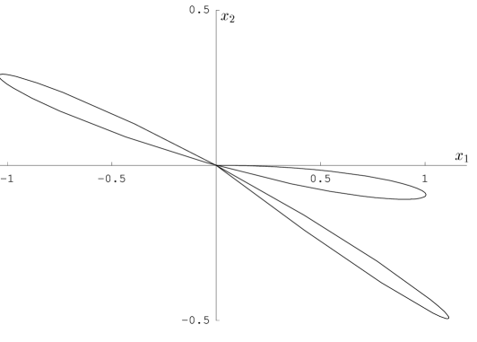
Figure 1: Trajectories for $r_{0}=0$ and $v_{0}=\Omega$, after three half-periods for $\kappa=20$, $\gamma=1.2$ and $m=5$. The ratio $\int_{0}^{\tau/2}({\dot{x}}_{1}x_{2}-{\dot{x}}_{2}x_{1})dt/{\cal E}=\pi\frac{\Gamma}{m\Omega^{3}}$ is preserved. ${\cal E}$ is the initial energy: ${\cal E}=\frac{1}{2}mv_{0}^{2}+\frac{1}{2}m\Omega^{2}r_{0}^{2}$.

We obtain dissquant :

$$\,{}_{H}\langle\psi(\tau)|\psi(0)\rangle_{H}=\,_{H_{{}_{I}}}\!\langle\psi(0)|\exp\left(i\int_{C_{0\tau}}A(t^{\prime})dt^{\prime}\right)|\psi(0)\rangle_{H_{{}_{I}}}\equiv e^{i\phi}\,,$$ (67)

where the contour $C_{0\tau}$ is the one going from $t^{\prime}=0$ to $t^{\prime}=\tau$ and back and $A(t)\equiv\frac{\Gamma m}{\hbar}({\dot{x}}_{1}x_{2}-{\dot{x}}_{2}x_{1})$. Note that $({\dot{x}}_{1}x_{2}-{\dot{x}}_{2}x_{1})dt$ is the area element in the $(x_{1},x_{2})$ plane enclosed by the trajectories (see Fig.1). Notice also that the evolution (or dynamical) part of the phase does not enter in $\phi$, as the integral in Eq.(67) picks up a purely geometric contribution Berry .

Because the physical states $|\psi\rangle$ are periodic ones, let us focus our attention on those. Following Berry , one may generally write

$$|\psi(\tau)\rangle = e^{i\phi-\frac{i}{\hbar}\int_{0}^{\tau}\langle\psi(t)|H|\psi(t)\rangle dt}|\psi(0)\rangle\,=\,e^{-i2\pi n}|\psi(0)\rangle\,,$$ (68)

i.e. $\frac{\langle\psi(\tau)|H|\psi(\tau)\rangle}{\hbar}\tau-\phi=2\pi n$, $n=0,1,2,\ldots$, which by using $\tau=\frac{2\pi}{\Omega}$ and $\phi=\alpha\pi$, gives

$${\cal H}_{{{}_{I}},e\!f\!f}^{n}\equiv\langle\psi_{n}(\tau)|H|\psi_{n}(\tau)\rangle=\hbar\Omega\left(n+\frac{\alpha}{2}\right)~{},$$ (69)

where the index $n$ has been introduced to exhibit the $n$ dependence of the state and the corresponding energy. ${\cal H}_{{\rm i},e\!f\!f}^{n}$ gives the effective $n$th energy level of the physical system, namely the energy given by ${\cal H}_{{\rm i}}^{n}$ corrected by its interaction with the environment. We thus see that the dissipation term $J_{2}$ of the Hamiltonian is actually responsible for the “zero point energy” ($n=0$): $E_{0}=\frac{\hbar}{2}\Omega\alpha$.

As well known, the zero point energy is the “signature” of quantization since in Quantum Mechanics it is formally due to the non-zero commutator of the canonically conjugate $q$ and $p$ operators. Thus dissipation manifests itself as “quantization”. In other words, $E_{0}$, which appears as the “quantum contribution” to the spectrum of the conservative evolution of physical states, signals the underlying dissipative dynamics. If we want to match the Quantum Mechanics zero point energy, we have to fix $\alpha=1$, which gives dissquant $\Omega=\frac{\gamma}{m}$.

5 Thermodynamics

In order to better understand the dynamical role of $J_{2}$ we rewrite Eq.(66) as

$$|\psi(t)\rangle_{H}={\hat{T}}\left[\exp\left(i\frac{1}{\hbar}\int_{u(t_{0})}^{u(t)}2J_{2}du^{\prime}\right)\right]|\psi(t)\rangle_{H_{{}_{I}}}\,,$$ (70)

by using $u(t)=-\Gamma t$. Accordingly, we have

$$-i\hbar\frac{\partial}{\partial u}|\psi(t)\rangle_{H}=2J_{2}|\psi(t)\rangle_{H}\,.$$ (71)

We thus see that $2J_{2}$ is responsible for shifts (translations) in the $u$ variable, as is to be expected since $2J_{2}=p_{u}$ (cf. Eq.(53)). In operatorial notation we can write indeed $p_{u}=-i\hbar\frac{\partial}{\partial u}$. Then, in full generality, Eq.(62) defines families of physical states, representing stable, periodic trajectories (cf. Eq.(63)). $2J_{2}$ implements transition from family to family, according to Eq.(71). Eq.(64) can be then rewritten as

$$i\hbar\frac{d}{dt}|\psi(t)\rangle_{H}=i\hbar\frac{\partial}{\partial t}|\psi(t)\rangle_{H}+i\hbar\frac{du}{dt}\frac{\partial}{\partial u}|\psi(t)\rangle_{H}\,,$$ (72)

where the first term on the r.h.s. denotes of course derivative with respect to the explicit time dependence of the state. The dissipation contribution to the energy is thus described by the “translations” in the $u$ variable. It is then interesting to consider the derivative

$$\frac{\partial S}{\partial U}=\frac{1}{T}\,.$$ (73)

From Eq.(57), by using $S\equiv\frac{2J_{2}}{\hbar}$ and $U\equiv 2\Omega{\cal C}$, we obtain $T=\hbar\Gamma$. Eq. (73) is the defining relation for temperature in thermodynamics (with $k_{B}=1$) so that one could formally regard $\hbar\Gamma$ (which dimensionally is an energy) as the temperature, provided the dimensionless quantity $S$ is identified with the entropy. In such a case, the “full Hamiltonian” Eq.(57) plays the role of the free energy ${\cal F}$: $H=2\Omega{\cal C}-(\hbar\Gamma)\frac{2J_{2}}{\hbar}=U-TS={\cal F}$. Thus $2\Gamma J_{2}$ represents the heat contribution in $H$ (or $\cal F$). Of course, consistently, $\left.\frac{\partial{\cal F}}{\partial T}\right|_{\Omega}=-\frac{2J_{2}}{\hbar}$. In conclusion $\frac{2J_{2}}{\hbar}$ behaves as the entropy, which is not surprising since it controls the dissipative (thus irreversible) part of the dynamics.

We can also take the derivative of ${\cal F}$ (keeping $T$ fixed) with respect to $\Omega$. We then have

$$\left.\frac{\partial{\cal F}}{\partial\Omega}\right|_{T}=\left.\frac{\partial U}{\partial\Omega}\right|_{T}=mr^{2}\Omega\,,$$ (74)

which is the angular momentum: this is to be expected since it is the conjugate variable of the angular velocity $\Omega$. It is also suggestive that the temperature $\hbar\Gamma$ is actually given by the background zero point energy: $\hbar\Gamma=\frac{\hbar\Omega}{2}$.

In the light of the above results, the condition (62) can be then interpreted as a condition for an adiabatic physical system. $\frac{2J_{2}}{\hbar}$ might be viewed as an analogue of the Kolmogorov–Sinai entropy for chaotic dynamical systems.

6 Conclusions

In this report we have reviewed some aspects of the quantization of the damped harmonic oscillator.

In the framework of the path integral formulation developed by Schwinger and by Feynman and Vernon, we have discussed the doubling of the phase-space degrees of freedom for dissipative systems and thermal field theories. We have shown how the doubled variables are related to quantum noise effects.

We have then discussed some algebraic features of the system of damped-antidamped harmonic oscillators which allows for a canonical treatment of quantum dissipation.

We also considered the relation of this model with the ’t Hooft proposal, according to which the loss of information due to dissipation in a classical deterministic system manifests itself in the quantum features of the system. We have shown that the quantum spectrum of the harmonic oscillator can be obtained from the dissipative character of the underlying deterministic system.

Finally, we have discussed the thermodynamical features of our system.

Acknowledgments

We would like to thank the organizers of the Piombino workshop DICE2002 on “Decoherence, Information, Complexity and Entropy” where some of the results contained in this report have been presented. We also thank the ESF network COSLAB, MIUR, INFN, INFM and EPSRC for partial support.

References

- (1) J. Schwinger: J. Math. Phys. 2 (1961), 407.
- (2) R.P. Feynman, F.L. Vernon: Annals Phys. 24, 118 (1963).
- (3) G. ’t Hooft: in “Basics and Highlights of Fundamental Physics”, Erice, (1999) [hep-th/0003005].
- (4) G. ’t Hooft: [hep-th/0104080]; [hep-th/0105105]; [quant-ph/0212095].
- (5) Y. Takahashi, H. Umezawa: Collective Phenomena 2, 55 (1975).
-
(6)
H.Umezawa: Advanced field theory: micro,
macro and thermal concepts (American Institute of Physics, N.Y.
1993);
H. Umezawa, M. Matsumoto, M. Tachiki: Thermo Field Dynamics and Condensed States (North-Holland, Amsterdam, 1982). - (7) E. Celeghini, M. Rasetti, G. Vitiello: Annals Phys. 215, 156 (1992).
- (8) M. Blasone, E. Graziano, O. K. Pashaev, G. Vitiello: Annals Phys. 252 115, (1996).
- (9) M. Blasone, P. Jizba: Can. J. Phys. 80, 645 (2002); [quant-ph/0102128].
- (10) Y. N. Srivastava, G. Vitiello, A. Widom: Annals Phys. 238, 200 (1995).
- (11) M. Blasone, Y. N. Srivastava, G. Vitiello, A. Widom: Annals Phys. 267, 61 (1998).
- (12) M. Blasone, P. Jizba, G. Vitiello: Phys. Lett. A 287, 205 (2001).
- (13) R. Banerjee: Mod. Phys Lett. A 17, 631 (2002); R. Banerjee, P. Mukherjee: J. Phys. A 35, 5591 (2002).
- (14) E. Alfinito, G. Vitiello: Class. Quant. Grav. 17, 93 (2000).
- (15) G. Vitiello: Int. J. Mod. Phys. B9, 973 (1995).
- (16) E. Alfinito, G. Vitiello: Int. J. Mod. Phys. B14, 853 (2000).
- (17) G. Vitiello: My Double Unveiled, (John Benjamins, Amsterdam 2001).
- (18) S. Sivasubramanian, Y. N. Srivastava, G. Vitiello, A. Widom: [quant-ph/0301005].
-
(19)
H. Bateman: Phys. Rev. 38, 815 (1931);
P. M. Morse, H. Feshbach: Methods of Theoretical Physics, Vol.I, pag. 298 (McGraw–Hill, New York, 1953);
H. Dekker: Phys. Rept. 80, 1 (1981). - (20) R. P. Feynman: Statistical Mechanics, (The Benjamin/Cummings Publ. Co., INC., Reading, Massachusetts, 1972).
- (21) H. Haken: Laser Theory Springer-Verlag, Berlin 1984.
- (22) B. G. Wybourne: Classical Groups in Physics, (John Wiley & Sons, Inc., London, 1974).
- (23) J. S. Bell, Speakable and unspeakable in Quantum Mechanics (Cambridge University Press, 1987).
- (24) H. T. Elze, O. Schipper: Phys. Rev. D 66, 044020 (2002).
- (25) M. Blasone, E. Celeghini, P. Jizba, G. Vitiello: [quant-ph/0208012].
- (26) J. Anandan, Y. Aharonov, Phys. Rev. Lett. 65, 1697 (1990).