Present Address: ]Dept. of Physics, Technion, Haifa ISRAEL Present Address: ]NIST Optoelectronics Division

Experimental demonstration of a technique to generate arbitrary quantum superposition states

Abstract

Using a single, harmonically trapped ⁹Be⁺ ion, we experimentally demonstrate a technique for generation of arbitrary states of a two-level particle confined by a harmonic potential. Rather than engineering a single Hamiltonian that evolves the system to a desired final sate, we implement a technique that applies a sequence of simple operations to synthesize the state.

The goal of deterministically synthesizing or “engineering” arbitrary states of a quantum system is at the heart of such diverse fields as quantum computation 1 and reaction control in chemistry 2 . For harmonic oscillator states, particular non-linear interactions can be used to generate special states such as squeezed states. However, it is intractable to realize a single interaction required to create an arbitrary state. Law and Eberly 3 have devised a technique for arbitrary harmonic oscillator state generation that couples the oscillator to a two-level atomic or “spin” system and applies a sequence of operations that use simple interactions. We demonstrate this technique on the harmonic motion of a single trapped ⁹Be⁺ ion and include the generation of arbitrary spin-oscillator states 4 . Such quantum state control is relevant to the scheme for constructing a quantum computer using trapped atomic ions 7 ; 8 , where we must control the quantized micro-mechanical system composed of the collective ion normal modes that are used as a data bus to transfer information between the ion qubits. These techniques could also be used to create input states for quantum computing schemes that use continuous variables 25 including the code-words that are required for fault tolerant computation 26 .

Arbitrary quantum state synthesis is difficult unless certain conditions are met. As an example, consider a simple quantum system with four energy eigenstates labelled $\left|0\right\rangle$, $\left|1\right\rangle$, $\left|2\right\rangle$, and $\left|3\right\rangle$. If the system is initially prepared in $\left|0\right\rangle$, and if couplings that create superpositions $\alpha_{i}\left|0\rangle+\beta_{i}\right|i\rangle$ ($i$ = 1,2,3) can selectively be turned on, then we can create arbitrary superpositions of the form $c_{0}\left|0\right\rangle+c_{1}\left|1\right\rangle+c_{2}\left|2\right\rangle+c_{3}\left|3\right\rangle$. Here, the $c_{i}$ are complex and subject to the usual normalization condition $\sum_{i}\left|c_{i}\right|^{2}=1$. This method could be realized in an atomic system if the four states were non-degenerate levels with different energy separations and coherent transitions $\left|0\right\rangle\leftrightarrow\left|i\right\rangle$ could be driven by applied radiation. These requirements are not often met in practice. For example, it may be impossible to realize all of the desired couplings $\left|0\right\rangle\leftrightarrow\left|i\right\rangle$. Also, if the eigenstates are equally spaced like the first four energy levels of a harmonic oscillator, then driving the $\left|0\right\rangle\leftrightarrow\left|1\right\rangle$ transition also induces successive transitions $\left|1\right\rangle\leftrightarrow\left|2\right\rangle$, $\left|2\right\rangle\leftrightarrow\left|3\right\rangle$, etc. leading to fixed relations between the $c_{i}$.

It has long been recognized that certain interactions can cause harmonic oscillators to evolve to particular desired states 9 . For example, if the oscillator is excited from its ground state with the nonlinear force $F_{0}z\cos(2\omega t)$ then a “vacuum-squeezed” state is created. Such states can be used to increase measurement precision in specific applications such as interferometry 10 . However, it is usually intractable to find the desired force or interaction that will create a state with arbitrary coefficients. To circumvent this problem, schemes have been proposed 11 ; 12 that sequentially couple atomic superposition states to the field of a cavity mode and statistically prepare arbitrary field states through projective measurements. An alternative method has been proposed to deterministically map a previously prepared superposition of atomic Zeeman states onto the field of a cavity 13 . A more general deterministic scheme to prepare arbitrary field states has been suggested by Law and Eberly 3 ; 14 . The idea relies on coupling the harmonic oscillator to an auxiliary two-level quantum system through a sequence of simple interactions.

Consider an auxiliary system consisting of two internal states of an atom which we label $\left|\downarrow\right\rangle$ and $\left|\uparrow\right\rangle$ in analogy with the two-level system resulting from a spin-$1/2$ magnetic moment in a magnetic field. In practice, the harmonic oscillator could correspond to a single mode of the radiation field 3 or the mechanical oscillation of a trapped atom 4 ; 15 . The combined energy levels for this system are depicted in Fig. 1. As an example, we summarize the procedure to create the state $\left|\downarrow\right\rangle\sum_{i=0...3}c_{\downarrow i}\left|i\right\rangle$ starting from the ground state $\left|\downarrow\right\rangle\left|0\right\rangle$. It is simplest to first think about solving the inverse problem 3 : creating the state $\left|\downarrow\right\rangle\left|0\right\rangle$ from the initial state $\left|\downarrow\right\rangle\sum_{i=0...3}c_{\downarrow i}\left|i\right\rangle$. The procedure begins by applying a resonant pulse of radiation that carries out a “$\pi$-pulse” $\left|\downarrow\right\rangle\left|3\right\rangle\rightarrow\left|\uparrow\right\rangle\left|2\right\rangle$ leaving no amplitude in the $\left|\downarrow\right\rangle\left|3\right\rangle$ state (“clearing it out”) and placing amplitude $c_{\downarrow 3}$ in the $\left|\uparrow\right\rangle\left|2\right\rangle$ state. Applying this radiation also causes transitions between other states $\left|\downarrow\right\rangle\left|n\right\rangle$ and $\left|\uparrow\right\rangle\left|n-1\right\rangle$. Because in general the coherent transition rates (Rabi rates) are not the same for different values of $n$ 18 , in this first step the amplitudes of the other states change according to $c_{\downarrow n}\left|\downarrow\right\rangle\left|n\right\rangle\rightarrow c^{\prime}_{\downarrow n}\left|\downarrow\right\rangle\left|n\right\rangle+d^{\prime}_{\uparrow,n-1}\left|\uparrow\right\rangle\left|n-1\right\rangle$. The Law/Eberly method succeeds because the state $\left|\downarrow\right\rangle\left|0\right\rangle$ remains unaffected since the state $\left|\uparrow\right\rangle\left|-1\right\rangle$ does not exist.

The second step is to induce the transition $c_{\downarrow 3}\left|\uparrow\right\rangle\left|2\right\rangle+c^{\prime}_{\downarrow 2}\left|\downarrow\right\rangle\left|2\right\rangle\rightarrow c^{\prime\prime}_{\downarrow 2}\left|\downarrow\right\rangle\left|2\right\rangle$, thereby clearing out the $\left|\uparrow\right\rangle\left|2\right\rangle$ state. The duration and phase of the second pulse are chosen according to the known values of $c_{\downarrow 3}$ and $c^{\prime}_{\downarrow 2}$ in order to collapse the superposition state. The first two steps have cleared out the $\left|\downarrow\right\rangle\left|3\right\rangle$ and $\left|\uparrow\right\rangle\left|2\right\rangle$ states but, in general, non-zero amplitudes remain in the $\left|\uparrow\right\rangle\left|0\right\rangle$, $\left|\uparrow\right\rangle\left|1\right\rangle$, $\left|\downarrow\right\rangle\left|0\right\rangle$, $\left|\downarrow\right\rangle\left|1\right\rangle$, and $\left|\downarrow\right\rangle\left|2\right\rangle$ states. However, by repeating this two-step clearing-out process for successively lower values of $n$, the state amplitudes are transferred down the dual ladder of states eventually to the ground state $\left|\downarrow\right\rangle\left|0\right\rangle$. Finally, to achieve the original goal, we apply these same steps in a time-reversed fashion to carry out the mapping to $\left|\downarrow\right\rangle\sum_{i=0...3}c_{\downarrow i}\left|i\right\rangle$. In the experiments described below, we demonstrate the Law/Eberly technique by implementing the mapping $\left|\downarrow\right\rangle\left|0\right\rangle\rightarrow\left|\downarrow\right\rangle\left(\left|0\right\rangle+\left|3\right\rangle\right)$ and other intermediate mappings of the form $\left|\downarrow\right\rangle\left|0\right\rangle\rightarrow\sum_{i}\left(c_{\downarrow i}\left|\downarrow\right\rangle+c_{\uparrow i}\left|\uparrow\right\rangle\right)\left|i\right\rangle$ 4 .

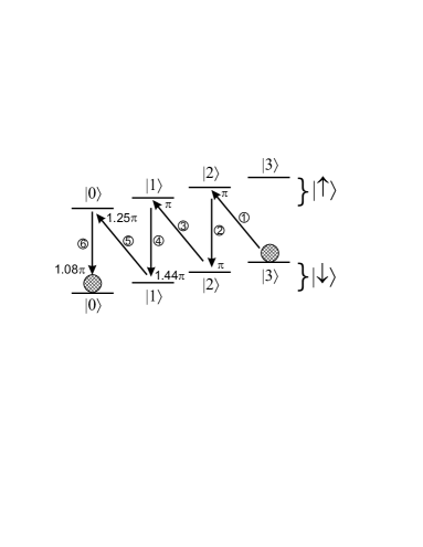
Figure 1: Schematic energy level diagram for the combined harmonic oscillator/spin-1/2 system (only harmonic oscillator levels with $n\leq 3$ are shown). The arrows show the laser pulse sequence used to generate the state $\left|\downarrow\right\rangle\left|0\right\rangle$ from the state $\left|\Psi_{03}\right\rangle=\left|\downarrow\right\rangle\left(\left|0\right\rangle+\left|3\right\rangle\right)/\sqrt{2}$. The laser pulses are applied in a stepwise fashion (labelled from 1 to 6) where the pulse areas $\Omega_{n,n^{\prime}}t$ (marked next to the head of each arrow) are calculated according to the Rabi rate for the numbered transitions. In this notation, a “$\pi$-pulse” would completely transfer all of the population from an initial state $\left|\downarrow\right\rangle\left|n\right\rangle$ to a final state $\left|\uparrow\right\rangle\left|n^{\prime}\right\rangle$, for example. To generate $\left|\Psi_{03}\right\rangle$ from $\left|\downarrow\right\rangle\left|0\right\rangle$, the pulse sequence shown here is applied in a time-reversed manner.

The harmonic oscillator and auxiliary levels in our experiment correspond to the motional and internal states of a single ⁹Be⁺ atomic ion trapped in a linear Paul trap 16 . We use the harmonic oscillator motional states along the trap axis ($z$ direction) which are equally spaced in energy by $h\times(2.9$ MHz), where $h$ is Planck’s constant. In this direction, the ion is confined by a static electric harmonic potential. The $\left|\uparrow\right\rangle$ and $\left|\downarrow\right\rangle$ (auxiliary) spin states are the $F=1,m_{F}=-1$ and $F=2,m_{F}=-2$ hyperfine levels of the ion’s ${}^{2}S_{1/2}$ electronic ground state, which are separated in energy by approximately $h\times(1250$ MHz). Applied laser radiation is used for state preparation and manipulation. A pair of laser beams detuned by approximately +80 GHz from the ${}^{2}S_{1/2}$ to ${}^{2}P_{1/2}$ electronic transition ($\lambda\sim 313$ nm) drives coherent Raman transitions and couples the $\left|\uparrow\right\rangle$ and $\left|\downarrow\right\rangle$ states and motional levels 8 ; 17 . Motion sensitive coupling is produced using non-collinear beams with a wavevector difference along $z$. The Raman laser beam frequency difference is tuned to drive $\left|\uparrow\right\rangle\left|n-\Delta n\right\rangle\leftrightarrow\left|\downarrow\right\rangle\left|n\right\rangle$ or $\left|\uparrow\right\rangle\left|n\right\rangle\leftrightarrow\left|\downarrow\right\rangle\left|n\right\rangle$ transitions, and the coherent transition rate, or Rabi frequency, depends on both $n$ and $\Delta n$ 18 ; 19 . The experimental observable is the atomic spin state which we detect through state-dependent resonance fluorescence measurements at the end of every experiment 8 ; 20 .

To demonstrate the Law/Eberly scheme, we configure the apparatus to generate the state $\left|\Psi_{03}\right\rangle=\left|\downarrow\right\rangle\left(\left|0\right\rangle+\left|3\right\rangle\right)/\sqrt{2}$ from $\left|\downarrow\right\rangle\left|0\right\rangle$ using only transitions $\left|\uparrow\right\rangle\left|n-\Delta n\right\rangle\leftrightarrow\left|\downarrow\right\rangle\left|n\right\rangle$ where $\Delta n$ alternates between 0 and 1. The ion is initialized in the $\left|\downarrow\right\rangle\left|0\right\rangle$ state with greater than 99.9% probability using stimulated Raman cooling and optical pumping 21 . The six steps required to carry out the reverse process (produce $\left|\downarrow\right\rangle\left|0\right\rangle$ from $\left|\Psi_{03}\right\rangle$) are calculated according to the step-wise algorithm and are shown in Fig. 1.

The state created after applying the Law/Eberly scheme is analyzed through measurements of Rabi oscillations on the $\left|\downarrow\right\rangle\left|n\right\rangle\leftrightarrow\left|\uparrow\right\rangle\left|n+\Delta n\right\rangle$, $\Delta n$=0,$\pm 1$ transitions 17 ; 23 . The probability $P_{\downarrow}=\sum_{i}\left|c_{\downarrow i}\right|^{2}$ to detect the ion in the $\left|\downarrow\right\rangle$ state is recorded after applying a laser pulse on one of these transitions for duration $t$. The observed oscillations (see Fig. 3) of $P_{\downarrow}$ as a function of the laser pulse duration are fit to a sum of cosine functions with Rabi frequencies $\Omega_{n,n+\Delta n}(=\Omega_{n+\Delta n,n})$ constrained by the measured ratio of Rabi frequencies for the different motional levels fitnote . The amplitude and phase (left as free parameters in the fit) of each frequency component are used to determine the probabilities $\left|c_{\uparrow i}\right|^{2}$ and $\left|c_{\downarrow i}\right|^{2}$ for $i=0,1,2,3$ fitnote2 . We find that the observed ion population corresponds to the target state with 0.89 probability (Table 1), and that the populations in $\left|\downarrow\right\rangle\left|0\right\rangle$ and $\left|\downarrow\right\rangle\left|3\right\rangle$ are equal within the 0.03 measurement uncertainty.

Figure 2: Measured Rabi oscillations for the target state $\left|\Psi_{03}\right\rangle$. The probability to measure the atom in the $\left|\downarrow\right\rangle$ state is determined after applying a laser pulse coupling states $\left|\downarrow\right\rangle\left|n\right\rangle\leftrightarrow\left|\uparrow\right\rangle\left|n+1\right\rangle$ for a variable length of time. Each data point (solid circles) represents the average of 600 experiments. The solid line is a fit to the data that is used to determine the populations in the first four motional states and the two spin states. Typically the fit determines that the $1/e$ time constant for the exponentially decaying envelope included in the fit corresponds to 9 oscillations for the $\left|\downarrow\right\rangle\left|0\right\rangle\leftrightarrow\left|\uparrow\right\rangle\left|1\right\rangle$ transition. The observed beating arises primarily from the oscillations of population in the $\left|\downarrow\right\rangle\left|0\right\rangle$ and $\left|\downarrow\right\rangle\left|3\right\rangle$ states, which have Rabi frequencies such that $\Omega_{34}/\Omega_{01}=0.60$. The uncertainty in the spin state discrimination is smaller than the scatter in the data, which is mainly due to laser intensity and magnetic field fluctuations.

	n=0	1	2	3
$\downarrow$	0.43	0	0.01	0.46
$\uparrow$	0.03	0.04	0.02	0.01

Table 1: Measured state populations for the experiment with the target state $\left|\Psi_{03}\right\rangle$. Data similar to that in Fig. 2 are used to determine the probability $P=|c_{m_{s},n}|^{2}$ to find the ion in the motional level $n$ and the spin state $m_{s}=\downarrow,\uparrow$ for the intended target state $\left|\Psi_{03}\right\rangle$. This table shows the average of populations determined from using Rabi oscillation measurements employing couplings with $\Delta n=0,\pm 1$. The uncertainty in the measured probabilities is 0.03 and is dominated by scatter in the Rabi oscillation data and the finite observation time.

The probabilities $\left|c_{\uparrow i}\right|^{2}$ and $\left|c_{\downarrow i}\right|^{2}$ are also measured after each step in the procedure to generate $\left|\Psi_{03}\right\rangle$ and are compared to the theoretical predictions in Fig. 3. The Hilbert space trajectory from the initial to final state is somewhat complicated, with probability appearing, at least temporarily, in the $\left|\downarrow\right\rangle\left|n=0,1,2,3\right\rangle$ and $\left|\uparrow\right\rangle\left|n=0,1,2\right\rangle$ states.

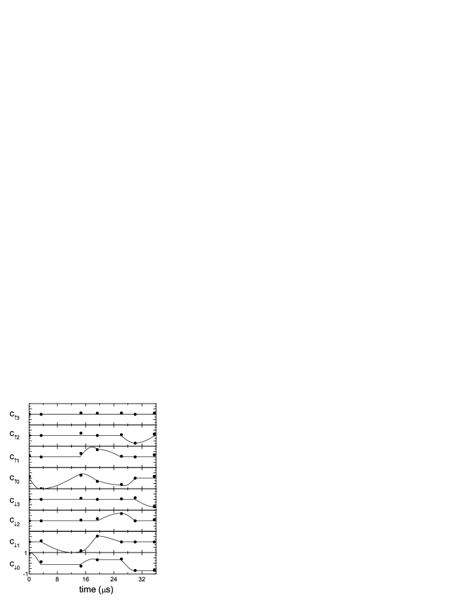
Figure 3: Initial to final state Hilbert space trajectory. The real amplitudes $c_{\downarrow n}$ and $c_{\uparrow n}$ are shown for the sequence used to generate $\left|\Psi_{03}\right\rangle$. The solid lines are the theoretical prediction, while the data (solid circles) are derived from the probabilities $|c_{\downarrow i}|^{2}$ and $|c_{\uparrow i}|^{2}$ measured using the Rabi oscillation technique after each step. The amplitude was determined by taking the square root of the measured probability and assigning a sign consistent with the final state and the length of the laser pulses.

The Rabi oscillation diagnostic determines the populations $\left|c_{\uparrow i}\right|^{2}$ and $\left|c_{\downarrow i}\right|^{2}$, but gives no information about the phase relation between the states. For example, measuring the populations in this way cannot distinguish between the pure (coherent superposition) state described by the density matrix $\rho=\left(\left|\downarrow\right\rangle\left|0\right\rangle+\left|\downarrow\right\rangle\left|3\right\rangle\right)\left(\right\langle 0\left|\right\langle\downarrow\left|+\right\langle 3\left|\right\langle\downarrow\left|\right)/2$ and the mixed (incoherent) state described by $\rho=\left(\left|\downarrow\right\rangle\left|0\right\rangle\right\langle 0\left|\right\langle\downarrow\left|+\left|\downarrow\right\rangle\left|3\right\rangle\right\langle 3\left|\right\langle\downarrow\left|\right)/2$. To verify that our implementation of the Law/Eberly scheme establishes coherence we have performed a test experiment starting from $\left|\downarrow\right\rangle\left|0\right\rangle$ using the target state $\left|\Psi_{T}\right\rangle=0.64\left|\downarrow\right\rangle\left|0\right\rangle+0.77\left|\uparrow\right\rangle\left|2\right\rangle$, which would give $\left|c_{\downarrow 0}\right|^{2}=0.41$ and $\left|c_{\uparrow 2}\right|^{2}=0.59$. The first five pulses of the $\left|\Psi_{03}\right\rangle$ sequence were used to generate $\left|\Psi_{T}\right\rangle$. The measured probabilities for the experimentally generated state were $\left|c_{\downarrow 0}\right|^{2}=0.39$, $\left|c_{\uparrow 2}\right|^{2}=0.55$, $\left|c_{\uparrow 0}\right|^{2}=0.03$, and 0.03 distributed among the remaining states.

A coherent analysis pulse was applied on $\left|\uparrow\right\rangle\left|n+2\right\rangle\leftrightarrow\left|\downarrow\right\rangle\left|n\right\rangle$ transitions after the $\left|\Psi_{T}\right\rangle$ state generation pulses but before spin state detection. The laser pulse area was adjusted to be a “$\pi/2$”-pulse for the $\left|\uparrow\right\rangle\left|2\right\rangle\leftrightarrow\left|\downarrow\right\rangle\left|0\right\rangle$ transition. For the pure $\left|\Psi_{T}\right\rangle$ state, the population would almost fully oscillate between the states $\left|\downarrow\right\rangle\left|0\right\rangle$ and $\left|\uparrow\right\rangle\left|2\right\rangle$ as the phase of the analysis pulse was varied relative to the state generation pulses. No sensitivity to this phase would be observed if the state we generated was an incoherent mixture of populations (dashed line in Fig. 4). The measured probability to find the atom in the state $\left|\downarrow\right\rangle$ as the laser phase is swept is shown in Fig. 4. The amplitude of these oscillations can be related to the fidelity

$$F = \langle\Psi_{T}|\rho\left|\Psi_{T}\right\rangle$$

$$= 0.41\rho_{\downarrow 0\downarrow 0}+0.59\rho_{\uparrow 2\uparrow 2}+0.495\left(\rho_{\downarrow 0\uparrow 2}+\rho_{\uparrow 2\downarrow 0}\right)$$

where $\rho$ is the experimentally measured density matrix. We determine that $F=0.93\pm 0.03$ using the measured populations and oscillation contrast to determine the relevant elements of the density matrix $\rho$ as in ref Sackett00 .

Figure 4: Coherence fringes. After generation pulses for the target state $0.64\left|\downarrow\right\rangle\left|0\right\rangle+0.77\left|\uparrow\right\rangle\left|2\right\rangle$ are implemented, a “$\pi/2$” analysis laser pulse is applied with a controlled phase relative to the state generation pulses. Shown here are the resulting oscillations in the probability $P_{\downarrow}$ to find the atom in the $\left|\downarrow\right\rangle$ state as the laser pulse phase is swept. The amplitude of the oscillation determined from a fit to a cosine function (solid line) is used to establish the fidelity of the experimentally generated state. The oscillation centered around $P_{\downarrow}=0.46$ is consistent with the measured probability in the $\left|\uparrow\right\rangle\left|0\right\rangle$ state (which is unaffected by the analysis laser coupling) and experimental error in the analysis laser pulse duration. The dashed line indicates the result if the prepared state is an incoherent mixture.

In summary, we have demonstrated experimentally the scheme of Law and Eberly 3 for generation of arbitrary harmonic-oscillator states and its extension 4 to arbitrary harmonic-oscillator/spin states. The method can be generalized to higher dimensions 4 , to the generation of arbitrary density matrices of harmonic oscillators 14 , to the creation of arbitrary motional observables 15 such as the phase 24 , and to the generation of arbitrary Zeeman state superpositions 29 . The precision with which we can implement this technique has a direct relation to the efficiency of quantum-information processing using trapped ions 7 . With sufficient improvements in the fidelity of such operations, one can contemplate using additional motional modes of motion as information carriers in this scheme. Of course, the same techniques can be applied in cavity-QED, the system in which it was originally conceived 3 . More generally, such techniques increase the variety of tools available for quantum-information processing and may eventually find application in areas not currently anticipated.

We thank D. Lucas and J. Ye for helpful comments on the manuscript. This work was supported by the NSA and the ARDA under Contract No. MOD-7171.00. Contribution of the U.S. Government: not subject to U.S. copyright.

References

(1) M. A. Nielsen and I. L. Chuang, Quantum Computation and
Quantum Information (Cambridge University Press, Cambridge,
2000).
(2) H. Rabitz, R. de Vivie-Riedle, M. Motzkus, and K. Kompa, Science 288, 824 (2000).
(3) C. K. Law and J. H. Eberly, Phys. Rev. Lett. 76, 1055 (1996).
(4) B. Kneer and C. K. Law, Phys. Rev. A 57, 2096 (1998).
(5) J. I. Cirac and P. Zoller, Phys. Rev. Lett. 74, 4091 (1995).
(6) C.A. Sackett, Quant. Inf. Comp. 1, 57 (2001).
(7) S. Lloyd and S.L. Braunstein, Phys. Rev. Lett. 82, 1784 (1999).
(8) D. Gottesman, A. Kitaev, and J. Preskill, Phys. Rev. A 64, 012310 (2001).
(9) See, for example, D. F. Walls and G. J. Milburn, Quantum Optics, (Springer,
Berlin, 1994).
(10) C. M. Caves, Phys. Rev. D 23, 1693 (1981); M. Xiao, L.-A. Wu, and H. J. Kimble, Phys. Rev. Lett. 59, 278 (1987).
(11) K. Vogel, V. M. Akulin, and W. P. Schleich, Phys. Rev. Lett. 71, 1816 (1993).
(12) B. M. Garraway, B. Sherman, H. Moya-Cessa, P. L. Knight, and
G. Kurizki, Phys. Rev. A 49, 535 (1994).
(13) A. S. Parkins, P. Marte, P. Zoller, and H. J. Kimble, Phys. Rev. Lett. 71, 3095 (1993).
(14) C. K. Law, J. H. Eberly, and B. Kneer, J. Mod. Opt.
44, 2149 (1997).
(15) S. A. Gardiner, J. I. Cirac, and P. Zoller, Phys. Rev. A 55, 1683 (1997).
(16) D. J. Wineland and W. M. Itano, Phys.
Rev. A 20, 1521 (1979).
(17) M.A. Rowe et al., Quant. Inf. Comp. 4, 257 (2002).
(18) D.M. Meekhof, C. Monroe, B.E. King, W.M. Itano, and D.J.
Wineland, Phys. Rev. Lett. 76, 1796 (1996).
(19) D. J. Wineland et al., J. Res. Natl.
Inst. Stand. Technol. 103, 579 (1998).
(20) M.A. Rowe et al., Nature 409, 791 (2001).
(21) C. Monroe, D.M. Meekhof, B.E. King, W.M. Itano, and D.J.
Wineland, Phys. Rev. Lett. 75, 4714 (1995).
(22) D. Leibfried, D.M. Meekhof, C. Monroe, B.E. King, W.M. Itano,
and D.J. Wineland, J. Mod. Optics 44, 2485 (1997).
(23) We include the possibility for population only
in the levels in the fits. We estimate that the
probability that ambient heating and off-resonant coupling to
other sideband transitions populates levels higher than
after the state generation pulses is less than 0.1%.
(24) The fit assumes phases of only 0 or
between coherent superposition amplitudes that remain between
coupled states. If other phases exist, the Rabi oscillation
contrast is reduced and we underestimate the populations. We
determine that, to a good approximation, other phases can be ruled
out because the sum of populations (left as a free parameter) sum
to unity within the fit uncertainty.
(25) C.A. Sackett et al., Nature 404,
256 (2000).
(26) S. M. Barnett and D. T. Pegg, Phys. Rev. Lett. 76, 4148 (1996).
(27) C.K. Law and J.H. Eberly, Opt. Exp. 9, 368
(1998).