Experimental implementation of generalized Grover’s algorithm of multiple marked states and its application

1.Introdution

Since the quantum searching algorithm was first proposed by Grover [1], several generalizations of the original algorithm have been developed [2]-[4]. The generalized algorithm that we will realize can be posed as follows. Let $N$ basis states of a system constitute set $D$. A function $F$ is defined as $F:D\rightarrow\{0,1\}$. The states satisfying $F(x)=1$ are defined as marked states, which constitute set $M$ with a total of $r$ states. The other states in $D$, satisfying $F(x)=0$, constitute set $\overline{M}$ with a total of $N-r$ states. The states in $M$ and $\overline{M}$ have amplitudes $k_{i}$ and $l_{i}$, respectively. A unitary operator $U$ transforms a predefined basis state $|s>$ into a superposition denoted as $|g(0)>=U|s>$. $U$ can be almost any valid quantum mechanical unitary operator. $|g(0)>$ is the initial state for the algorithm. The phase rotation of marked states is described by $I_{t}^{\gamma}=\sum_{x}e^{i\gamma F(x)}|x><x|$. Obviously, if $|x>\in M$, $I_{t}^{\gamma}|x>=e^{i\gamma}|x>$; if $|x>\in\overline{M}$, $I_{t}^{\gamma}|x>=|x>$. A composite operator is defined as $G\equiv-UI_{s}^{\beta}U^{{\dagger}}$. $I_{s}^{\beta}$ is defined as $I_{s}^{\beta}\equiv I-(1-e^{i\beta})|s><s|$, where $I$ denotes unit matrix. The problem is to transform $|g(0)>$ to a target state denoted as $|\psi_{t}>=\sum_{i\in M}k_{i}|i>$ by repeating Grover iteration $n$ times. When the system lies in $|\psi_{t}>$, measurement yields $|k_{i}|^{2}$, the probability of the system being in marked state $|i>$. When $\beta=\pi$, $\gamma=\pi$, $|s>=|\overline{0}>$, and $U$ is chosen as Walsh-Hadamard (W-H) transform, the generalized algorithm becomes the original Grover’s algorithm, where $|\overline{0}>$ denotes all qubits in the 0 state.

E.Biham et al have analyzed generalized Grover’s algorithm using recursion equations [3]. Through introducing an ancilla qubit and choosing a proper $U$, Grover proposed a theoretical scheme to synthesize a specified quantum superposition on $N$ states in $O(\sqrt{N})$ steps using the algorithm [5]. We find that some special superpositions, such as EPR states, can be synthesized using the algorithm without the ancilla qubit. Generalized Grover’s algorithm of one marked state has been realized on a two-qubit NMR quantum computer. G.-L. Long et al realized the algorithm by choosing the phase rotation as $I_{t}^{\frac{\pi}{2}}$, while the W-H transform is retained [6]. In our previous work, we realized the algorithm by replacing the W-H transform by other unitary operator, while the $\pi$ phase rotation ($I_{t}^{\pi}$) was unaltered [7]. In this paper, we will realize the generalized algorithm of multiple marked states and synthesize EPR states. The W-H transform is replaced by other unitary operator and the phase rotation is chosen as $I_{t}^{\frac{\pi}{2}}$ or $I_{t}^{-\frac{\pi}{2}}$.

2.The generalized Grover’s algorithm

In this section, we will use some results in Ref.[3] to express the principle of our experiments.

$n$ applications of $GI_{t}^{\gamma}$ transform $|g(0)>$ into $|g(n)>$, described by

$$|g(n)>=\sum_{i\in M}k_{i}(n)|i>+\sum_{i\in\overline{M}}l_{i}(n)|i>.$$ (1)

When $n=0$, the system lies in the initial state

$$|g(0)>=U|s>.$$ (2)

One can find that $k_{i}(0)=U_{is}$, $i\in M$, and $l_{i}(0)=U_{is}$, $i\in\overline{M}$, where $U_{is}=<i|U|s>$. $GI_{t}^{\gamma}$ transforms the amplitudes $k_{j}(n)$, $j\in M$, to $k_{j}(n+1)=<j|GI_{t}^{\gamma}|g(n)>$ and amplitudes $l_{j}(n)$, $j\in\overline{M}$ to $l_{j}(n+1)=<j|GI_{t}^{\gamma}|g(n)>$. The recursion equations describing such iteration are expressed as

$$k_{j}(n+1)=e^{i\gamma}(1-e^{i\beta})U_{js}\sum_{i\in M}k_{i}(n)U_{is}^{*}+(1-e^{i\beta})U_{js}\sum_{i\in\overline{M}}l_{i}(n)U_{is}^{*}-e^{i\gamma}k_{j}(n),$$ (3)

$$l_{j}(n+1)=e^{i\gamma}(1-e^{i\beta})U_{js}\sum_{i\in M}k_{i}(n)U_{is}^{*}+(1-e^{i\beta})U_{js}\sum_{i\in\overline{M}}l_{i}(n)U_{is}^{*}-l_{j}(n).$$ (4)

Without loss of generality, we assume that $U_{is}\neq 0$, $i=1,2,\cdots$. Valuables $k_{i}^{{}^{\prime}}(n)$ and $l_{i}^{{}^{\prime}}(n)$ are defined as

$$k_{i}^{{}^{\prime}}(n)=\frac{k_{i}(n)}{U_{is}},$$ (5)

$$l_{i}^{{}^{\prime}}(n)=\frac{l_{i}(n)}{U_{is}}.$$ (6)

One can easily find that $k_{i}^{{}^{\prime}}(0)=1$, $l_{i}^{{}^{\prime}}(0)=1$. The weighted averages are defined as

$$\overline{k^{{}^{\prime}}}(n)=\frac{1}{W_{k}}\sum_{i\in M}|U_{is}|^{2}k_{i}^{{}^{\prime}}(n),$$ (7)

$$\overline{l^{{}^{\prime}}}(n)=\frac{1}{W_{l}}\sum_{i\in\overline{M}}|U_{is}|^{2}l_{i}^{{}^{\prime}}(n),$$ (8)

where $W_{k}=\sum_{i\in M}|U_{is}|^{2}$, and $W_{l}=\sum_{i\in\overline{M}}|U_{is}|^{2}$. With these variables, the recursion equations can be rewritten as

$$k_{j}^{{}^{\prime}}(n+1)=e^{i\gamma}(1-e^{i\beta})W_{k}\overline{k^{{}^{\prime}}}(n)+(1-e^{i\beta})W_{l}\overline{l^{{}^{\prime}}}(n)-e^{i\gamma}k_{j}^{{}^{\prime}}(n),$$ (9)

$$l_{j}^{{}^{\prime}}(n+1)=e^{i\gamma}(1-e^{i\beta})W_{k}\overline{k^{{}^{\prime}}}(n)+(1-e^{i\beta})W_{l}\overline{l^{{}^{\prime}}}(n)-l_{j}^{{}^{\prime}}(n).$$ (10)

By averaging over all the marked states in Eq.(9) and over all the unmarked states in Eq.(10), we find the two recursion equations for $\overline{k^{{}^{\prime}}}(n)$ and $\overline{l^{{}^{\prime}}}(n)$ can be expressed as

$$\overline{k^{{}^{\prime}}}(n+1)=e^{i\gamma}(1-e^{i\beta})W_{k}\overline{k^{{}^{\prime}}}(n)+(1-e^{i\beta})W_{l}\overline{l^{{}^{\prime}}}(n)-e^{i\gamma}\overline{k^{{}^{\prime}}}(n),$$ (11)

$$\overline{l^{{}^{\prime}}}(n+1)=e^{i\gamma}(1-e^{i\beta})W_{k}\overline{k^{{}^{\prime}}}(n)+(1-e^{i\beta})W_{l}\overline{l^{{}^{\prime}}}(n)-\overline{l^{{}^{\prime}}}(n).$$ (12)

Subtracting Eq.(11) from Eq.(9), and Eq.(12) from Eq.(10), one finds that

$$k_{j}^{{}^{\prime}}(n+1)-\overline{k^{{}^{\prime}}}(n+1)=-e^{i\gamma}(k_{j}^{{}^{\prime}}(n)-\overline{k^{{}^{\prime}}}(n)),$$ (13)

$$l_{j}^{{}^{\prime}}(n+1)-\overline{l^{{}^{\prime}}}(n+1)=-(l_{j}^{{}^{\prime}}(n)-\overline{l^{{}^{\prime}}}(n)).$$ (14)

Noting that $k_{i}^{{}^{\prime}}(0)=1$, $l_{i}^{{}^{\prime}}(0)=1$, we find $\overline{k^{{}^{\prime}}}(0)=1$, $\overline{l^{{}^{\prime}}}(0)=1$. Using Eqs.(13) and (14), we obtained

$$k_{i}^{{}^{\prime}}(n)=\overline{k^{{}^{\prime}}}(n),$$ (15)

$$l_{i}^{{}^{\prime}}(n)=\overline{l^{{}^{\prime}}}(n),$$ (16)

where the subscript $j$ in Eqs.(13) and (14) has been replaced by $i$.

From the discussion above, for any $U$, $\overline{k^{{}^{\prime}}}(n)$ and $\overline{l^{{}^{\prime}}}(n)$ can be solved from Eqs. (11) and (12). Using Eqs.(15),(16),(5),and (6), we can obtain the explicit expressions for $k_{i}(n)$ and $l_{i}(n)$. Eqs.(11) and (12) can be rewritten as

$$\left(\begin{array}[]{cc}\overline{k^{{}^{\prime}}}(n+1)\\ \overline{l^{{}^{\prime}}}(n+1)\end{array}\right)=A\left(\begin{array}[]{cc}\overline{k^{{}^{\prime}}}(n)\\ \overline{l^{{}^{\prime}}}(n)\end{array}\right),$$ (17)

where

$$A=\left(\begin{array}[]{cc}e^{i\gamma}(1-e^{i\beta})W_{k}-e^{i\gamma}&(1-e^{i\beta})W_{l}\\ e^{i\gamma}(1-e^{i\beta})W_{k}&(1-e^{i\beta})W_{l}-1\end{array}\right).$$ (18)

Eq.(17) shows that $\overline{k^{{}^{\prime}}}(n)$ and $\overline{l^{{}^{\prime}}}(n)$ are dependent on $\gamma$, $\beta$, and $|U_{is}|$. If $U$ is replaced by a different $U^{\prime}$ where $|U^{\prime}_{is}|=|U_{is}|$, the analysic forms of $\overline{k^{{}^{\prime}}}(n)$ and $\overline{l^{{}^{\prime}}}(n)$ are unaltered. If $l_{i}(n)$ approaches 0 when $n=n_{0}$, the system lies in

$$|\psi_{t}>=\sum_{i\in M}U_{is}\overline{k^{{}^{\prime}}}(n_{0})|i>.$$ (19)

Generally, the state is not the equally weighted superposition of marked states. It is related to $U_{is}$. By choosing proper $U$, some superpositions can be synthesized using generalized Grover’s algorithm. We will solve Eq.(17) in the following section.

3.Experimental scheme

Our experiments use a sample of Carbon-13 labelled chloroform dissolved in d6-acetone. Data are taken at room temperature with a Bruker DRX 500 MHz spectrometer. The resonance frequencies $\nu_{1}=125.76$ MHz for ${}^{13}C$, and $\nu_{2}=500.13$ MHz for ${}^{1}H$. The coupling constant $J$ is measured to be 215 Hz. If the magnetic field is along $\hat{z}$-axis, and let $\hbar=1$, the Hamitonian of this system is described by

$$H=-2\pi\nu_{1}I_{z}^{1}-2\pi\nu_{2}I_{z}^{2}+2\pi JI_{z}^{1}I_{z}^{2},$$ (20)

where $I_{z}^{k}(k=1,2)$ are the matrices for $\hat{z}$-component of the angular momentum of the spins [8]. In the rotating frame of spin $k$, the evolution caused by a radio-frequency(rf) pulse on resonance along $\hat{x}$ or $-\hat{y}$-axis is denoted as $X_{k}(\varphi_{k})=e^{i\varphi_{k}I_{x}^{k}}$ or $Y_{k}(-\varphi_{k})=e^{-i\varphi_{k}I_{y}^{k}}$, where $\varphi_{k}=B_{1}\gamma_{k}t_{p}$ with $k$ specifying the affected spin. $B_{1}$, $\gamma_{k}$ and $t_{p}$ represent the strength of rf pulse, gyromagnetic ratio and the width of rf pulse, respectively. The pulse used above is denoted as $[\varphi]_{x}^{k}$ or $[-\varphi]_{y}^{k}$. The coupled-spin evolution is denoted as

$$[t]=e^{-i2\pi JI_{z}^{1}I_{z}^{2}},$$ (21)

where $t$ is evolution time. The predefined pseudo-pure state

$$|s>=|\uparrow>_{1}|\uparrow>_{2}=\left(\begin{array}[]{c}1\\ 0\\ 0\\ 0\end{array}\right)$$ (22)

is prepared by using spatial averaging [9], where $|\uparrow>_{k}$ denotes the state of spin $k$. For convenience, the notation $|\uparrow>_{1}|\uparrow>_{2}$ is simplified as $|\uparrow\uparrow>$. The basis states are arrayed as $|\uparrow\uparrow>,|\uparrow\downarrow>,|\downarrow\uparrow>$, $|\downarrow\downarrow>$. $U$ is chosen as $U=Y_{1}(\varphi_{1})Y_{2}(\varphi_{2})$ represented as

$$U=\left(\begin{array}[]{cccc}c_{1}c_{2}&c_{1}s_{2}&s_{1}c_{2}&s_{1}s_{2}\\ -c_{1}s_{2}&c_{1}c_{2}&-s_{1}s_{2}&s_{1}c_{2}\\ -s_{1}c_{2}&-s_{1}s_{2}&c_{1}c_{2}&c_{1}s_{2}\\ s_{1}s_{2}&-s_{1}c_{2}&-c_{1}s_{2}&c_{1}c_{2}\end{array}\right),$$ (23)

where $c_{k}\equiv cos(\varphi_{k}/2)$, $s_{k}\equiv sin(\varphi_{k}/2)$. When $|\uparrow\uparrow>$ and $|\downarrow\downarrow>$ are the two marked states, $U$ can be chosen as $U=Y_{1}(\frac{\pi}{2})Y_{2}(\frac{\pi}{2})$ described by

$$U=\frac{1}{2}\left(\begin{array}[]{cccc}1&1&1&1\\ -1&1&-1&1\\ -1&-1&1&1\\ 1&-1&-1&1\end{array}\right).$$ (24)

One can find that $W_{k}=W_{l}=\frac{1}{2}$. When $\gamma=\beta=-\frac{\pi}{2}$, $I_{t}^{\gamma}$ and $I_{s}^{\beta}$ can be represented as

$$I_{14}^{-\frac{\pi}{2}}=\left(\begin{array}[]{cccc}-i&0&0&0\\ 0&1&0&0\\ 0&0&1&0\\ 0&0&0&-i\end{array}\right),$$ (25)

$$I_{s}^{-\frac{\pi}{2}}=\left(\begin{array}[]{cccc}-i&0&0&0\\ 0&1&0&0\\ 0&0&1&0\\ 0&0&0&1\end{array}\right).$$ (26)

Using the values of $\beta$, $\gamma$, $W_{k}$, and $W_{l}$, Eq.(18) is expressed by

$$A=\frac{1}{2}\left(\begin{array}[]{cc}1+i&1+i\\ 1-i&i-1\end{array}\right)$$ (27)

In order to obtain explicit expressions for $\overline{k^{{}^{\prime}}}(n)$ and $\overline{l^{{}^{\prime}}}(n)$, we introduce the diagonal matrix represented as

$$A_{D}=S^{-1}AS\equiv\left(\begin{array}[]{cc}\lambda_{+}&0\\ 0&\lambda_{-}\end{array}\right)$$ (28)

The eigenvalues of matrix $A$ are the solutions of $\det(A-\lambda I)=0$. They are expressed as $\lambda_{+}=e^{i\frac{\pi}{6}}$ , $\lambda_{-}=e^{i\frac{5\pi}{6}}$. $S$ and $S^{-1}$ are expressed as

$$S=\left(\begin{array}[]{cc}1&1\\ \frac{\sqrt{3}-1}{1+i}&-\frac{\sqrt{3}+1}{1+i}\end{array}\right),$$ (29)

$$S^{-1}=\left(\begin{array}[]{cc}\frac{\sqrt{3}+1}{2\sqrt{3}}&\frac{1+i}{2\sqrt{3}}\\ \frac{\sqrt{3}-1}{2\sqrt{3}}&-\frac{1+i}{2\sqrt{3}}\end{array}\right).$$ (30)

The solution of Eq.(17) can be expressed as

$$\left(\begin{array}[]{cc}\overline{k^{{}^{\prime}}}(n)\\ \overline{l^{{}^{\prime}}}(n)\end{array}\right)=A^{n}\left(\begin{array}[]{cc}\overline{k^{{}^{\prime}}}(0)\\ \overline{l^{{}^{\prime}}}(0)\end{array}\right),$$ (31)

where $A^{n}=SA_{D}^{n}S^{-1}$, expressed as

$$A^{n}=\frac{1}{2\sqrt{3}}\left(\begin{array}[]{cc}(\sqrt{3}+1)e^{i\frac{n\pi}{6}}+(\sqrt{3}-1)e^{i\frac{5n\pi}{6}}&(1+i)(e^{i\frac{n\pi}{6}}-e^{i\frac{5n\pi}{6}})\\ (1-i)(e^{i\frac{n\pi}{6}}-e^{i\frac{5n\pi}{6}})&(\sqrt{3}-1)e^{i\frac{n\pi}{6}}+(\sqrt{3}+1)e^{i\frac{5n\pi}{6}}\end{array}\right).$$ (32)

When $n=1$, we obtain that $\overline{k^{{}^{\prime}}}(1)=\sqrt{2}e^{i\frac{\pi}{4}}$, and $\overline{l^{{}^{\prime}}}(1)=0$. Using $U_{11}=\frac{1}{2}$, $U_{41}=\frac{1}{2}$, we obtain that $k_{1}(1)=e^{i\frac{\pi}{4}}/\sqrt{2}$, and $k_{4}(1)=e^{i\frac{\pi}{4}}/\sqrt{2}$. The system lies in state

$$|\psi_{1}>=(|\uparrow\uparrow>+|\downarrow\downarrow>)e^{i\frac{\pi}{4}}/\sqrt{2}.$$ (33)

The overall phase can be ignored.

If $U$ is chosen as $U=Y_{1}(-\frac{\pi}{2})Y_{2}(\frac{\pi}{2})$, Eq.(32) is unaltered. We also obtain $\overline{k^{{}^{\prime}}}(1)=\sqrt{2}e^{i\frac{\pi}{4}}$, and $\overline{l^{{}^{\prime}}}(1)=0$. Noting that $U_{11}=\frac{1}{2}$, and $U_{41}=-\frac{1}{2}$, we obtain that $k_{1}(1)=e^{i\frac{\pi}{4}}/\sqrt{2}$, and $k_{4}(1)=-e^{i\frac{\pi}{4}}/\sqrt{2}$. The system lies state

$$|\psi_{2}>=(|\uparrow\uparrow>-|\downarrow\downarrow>)e^{i\frac{\pi}{4}}/\sqrt{2}.$$ (34)

Considering the experimental convenience, if the marked states are $|\uparrow\downarrow>$ and $|\downarrow\uparrow>$, we choose $I_{t}^{\gamma}$ as $I_{23}^{\gamma}=iI_{14}^{-\frac{\pi}{2}}$, where $\gamma=\frac{\pi}{2}$. In matrix notation, $I_{23}^{\gamma}$ is represented as

$$I_{23}^{\frac{\pi}{2}}=\left(\begin{array}[]{cccc}1&0&0&0\\ 0&i&0&0\\ 0&0&i&0\\ 0&0&0&1\end{array}\right).$$ (35)

$\beta$ is changed to $\frac{\pi}{2}$ to satisfy phase matching [10]. $I_{s}^{\frac{\pi}{2}}$ is described by

$$I_{s}^{\frac{\pi}{2}}=\left(\begin{array}[]{cccc}i&0&0&0\\ 0&1&0&0\\ 0&0&1&0\\ 0&0&0&1\end{array}\right).$$ (36)

When $\gamma=\beta=\frac{\pi}{2}$, and $U=Y_{1}(\frac{\pi}{2})Y_{2}(\frac{\pi}{2})$, or $U=Y_{1}(-\frac{\pi}{2})Y_{2}(\frac{\pi}{2})$, the solution of Eq.(17) can be obtained by replacing $i$ in Eqs.(27)-(32) by $-i$. We obtain $\overline{k^{{}^{\prime}}}(1)=\sqrt{2}e^{-i\frac{\pi}{4}}$, and $\overline{l^{{}^{\prime}}}(1)=0$. When $U=Y_{1}(\frac{\pi}{2})Y_{2}(\frac{\pi}{2})$, we obtain $k_{2}(1)=-e^{-i\frac{\pi}{4}}/\sqrt{2}$, and $k_{3}(1)=-e^{-i\frac{\pi}{4}}/\sqrt{2}$, using $U_{21}=-\frac{1}{2}$, and $U_{31}=-\frac{1}{2}$. The system lies in state

$$|\psi_{3}>=-(|\uparrow\downarrow>+|\downarrow\uparrow>)e^{-i\frac{\pi}{4}}/\sqrt{2}.$$ (37)

Similarly, when $U=Y_{1}(-\frac{\pi}{2})Y_{2}(\frac{\pi}{2})$, we obtain $k_{2}(1)=-e^{-i\frac{\pi}{4}}/\sqrt{2}$, and $k_{3}(1)=e^{-i\frac{\pi}{4}}/\sqrt{2}$, using $U_{21}=-\frac{1}{2}$, and $U_{31}=\frac{1}{2}$. The system lies in state

$$|\psi_{4}>=-(|\uparrow\downarrow>-|\downarrow\uparrow>)e^{-i\frac{\pi}{4}}/\sqrt{2}.$$ (38)

$|\psi_{1}>$, $|\psi_{2}>$, $|\psi_{3}>$ and $|\psi_{4}>$ are the four EPR states. They are very useful in quantum information and have been implemented in experiments [11][12]. Based on the discussion above, they can be synthesized by generalized Grover’s algorithm. Other entangled states can be obtained by choosing other $U$. For example, if $U$ is chosen as

$$U=X_{1}(\frac{\pi}{2})Y_{2}(\frac{\pi}{2})=\frac{1}{2}\left(\begin{array}[]{cccc}1&1&i&i\\ -1&1&-i&i\\ i&i&1&1\\ -i&i&-1&1\end{array}\right),$$ (39)

and $\gamma=\beta=-\frac{\pi}{2}$, entangled state $(|\uparrow\uparrow>-i|\downarrow\downarrow>)e^{i\frac{\pi}{4}}/\sqrt{2}$ is obtained after one iteration. The target states, such as $|\psi_{1}>$ and $|\psi_{2}>$, can also be obtained by matrix multiplication. If replacing $n$ in Eq.(32) by $n+3$, one finds $A^{n+3}=iA^{n}$. This fact shows that $\overline{k^{{}^{\prime}}}(n)$ and $\overline{l^{{}^{\prime}}}(n)$ both have a period of 3.

4.Experimental procedure

The equilibrium density matrix can be represented as

$$\rho_{eq}=\gamma_{1}I_{z}^{1}+\gamma_{2}I_{z}^{2}.$$ (40)

The rf and gradient pulse sequence $[\alpha]_{x}^{2}-[grad]_{z}-[\pi/4]_{x}^{1}-1/4J-[\pi]_{x}^{1,2}-1/4J-[-\pi]_{x}^{1,2}-[-\pi/4]_{y}^{1}-[grad]_{z}$ transforms the system from the equilibrium state into the state represented as

$$\rho_{s}=I_{z}^{1}/2+I_{z}^{2}/2+I_{z}^{1}I_{z}^{2}=\frac{1}{4}\left(\begin{array}[]{cccc}3&0&0&0\\ 0&-1&0&0\\ 0&0&-1&0\\ 0&0&0&-1\end{array}\right),$$ (41)

which can be used as the pseudo-pure state $|\uparrow\uparrow>$ [13]. $\alpha=\arccos(\gamma_{1}/2\gamma_{2})$, $[grad]_{z}$ denotes gradient pulse along $\hat{z}$-axis, and the symbol 1/4J means that the system evolutes under $H$ described as Eq.(20) for 1/4J time when pulses are closed. The pulses are applied from left to right. $[\pi]_{x}^{1,2}$ denotes a nonselective pulse (hard pulse). The evolution caused by the pulse sequence $1/4J-[\pi]_{x}^{1,2}-1/4J-[-\pi]_{x}^{1,2}$ is equivalent to the coupled-spin evolution $[1/2J]$ described in Eq.(21) [14]. $\pi$ pulses are applied in pairs each of which take opposite phases in order to reduce the error accumulation caused by imperfect calibration of $[\pi]$ pulses [15]. $U$ is realized by $[\pm\pi/2]_{y}^{1}-[\pi/2]_{y}^{2}$, corresponding to $Y_{1}(\pm\frac{\pi}{2})Y_{2}(\frac{\pi}{2})$, respectively. Because $I_{23}^{\frac{\pi}{2}}=iI_{14}^{-\frac{\pi}{2}}$, $I_{23}^{\frac{\pi}{2}}$ and $I_{14}^{-\frac{\pi}{2}}$ can be realized by the same sequence $1/4J-[\pi]_{x}^{1,2}-1/4J-[-\pi]_{x}^{1,2}$. By modifying the pulses used in Refs.[6][16], we realize $I_{s}^{-\frac{\pi}{2}}$ by $1/8J-[\pi]_{x}^{1,2}-1/8J-[-\pi]_{x}^{1,2}-[-\pi/2]_{y}^{1,2}-[-\pi/4]_{x}^{1,2}-[\pi/2]_{y}^{1,2}$, and $I_{s}^{\frac{\pi}{2}}$ by $15/8J-[\pi]_{x}^{1,2}-15/8J-[-\pi]_{x}^{1,2}-[-\pi/2]_{y}^{1,2}-[\pi/4]_{x}^{1,2}-[\pi/2]_{y}^{1,2}$. When $U=Y_{1}(\frac{\pi}{2})Y_{2}(\frac{\pi}{2})$, $(-UI_{s}^{-\frac{\pi}{2}}U^{{\dagger}}I_{14}^{-\frac{\pi}{2}})U$ transforms the pseudo-pure state $|\uparrow\uparrow>$ into state $|\psi_{1}>$, and $(-UI_{s}^{\frac{\pi}{2}}U^{{\dagger}}I_{23}^{\frac{\pi}{2}})U$ transforms $|\uparrow\uparrow>$ into $|\psi_{3}>$, where $U$ transforms $|\uparrow\uparrow>$ into the initial state $|g(0)>$, and $()$ indicates Grover iteration. When $U=Y_{1}(-\frac{\pi}{2})Y_{2}(\frac{\pi}{2})$, $(-UI_{s}^{-\frac{\pi}{2}}U^{{\dagger}}I_{14}^{-\frac{\pi}{2}})U$ transforms $|\uparrow\uparrow>$ into $|\psi_{2}>$, and $(-UI_{s}^{\frac{\pi}{2}}U^{{\dagger}}I_{23}^{\frac{\pi}{2}})U$ transforms $|\uparrow\uparrow>$ into $|\psi_{4}>$. The results are expressed by density matrixes. For example, the density matrix corresponding to $|\psi_{1}>$ is represented as

$$\rho_{1}=(I_{x}^{1}I_{x}^{2}-I_{y}^{1}I_{y}^{2}+I_{z}^{1}I_{z}^{2})=\left(\begin{array}[]{cccc}0.25&0&0&0.5\\ 0&-0.25&0&0\\ 0&0&-0.25&0\\ 0.5&0&0&0.25\end{array}\right),$$ (42)

which is equivalent to $|\psi_{1}><\psi_{1}|$. A readout pulse $[\pi/2]_{y}^{2}$ transforms $\rho_{1}$ into $\rho_{1r}$ represented as

$$\rho_{1r}=\frac{1}{4}\left(\begin{array}[]{cccc}0&-1&1&1\\ -1&0&-1&-1\\ 1&-1&0&1\\ 1&-1&1&0\end{array}\right).$$ (43)

The information on matrix elements (1,3) and (2,4) in Eq.(43) can be directly obtained in the carbon spectrum, and the information on elements (1,2) and (3,4) can be directly obtained in the proton spectrum. Similarly, when the system lies in $|\psi_{2}>$, $|\psi_{3}>$, or $|\psi_{4}>$, the readout pulse $[\pi/2]_{y}^{2}$ transforms the system into the state represented as

$$\rho_{2r}=\frac{1}{4}\left(\begin{array}[]{cccc}0&-1&-1&-1\\ -1&0&1&1\\ -1&1&0&1\\ -1&1&1&0\end{array}\right),$$ (44)

$$\rho_{3r}=\frac{1}{4}\left(\begin{array}[]{cccc}0&1&1&-1\\ 1&0&1&-1\\ 1&1&0&-1\\ -1&-1&-1&0\end{array}\right),$$ (45)

or

$$\rho_{4r}=\frac{1}{4}\left(\begin{array}[]{cccc}0&1&-1&1\\ 1&0&-1&1\\ -1&-1&0&-1\\ 1&1&-1&0\end{array}\right).$$ (46)

Through observing the matrix elements (1,3), (2,4), (1,2) and (3,4) in Eqs.(43)-(46), one can distinguish the four EPR states.

5.Results

In experiments, for each target state, the carbon spectrum and proton spectrum are recorded in two experiments. For different target states, carbon spectra or proton spectra are recorded in an identical fashion. Because the absolute phase of an NMR signal is not meaningful, we must use reference signals to adjust carbon spectra and proton spectra so that the relative phases of the signals are meaningful [17]. When the system lies in the pseudo-pure state described as Eq.(41), the readout pulses $[\pi/2]_{y}^{1}$ and $[\pi/2]_{y}^{2}$ transform it into states represented as

$$\rho_{sr1}=\frac{1}{4}\left(\begin{array}[]{cccc}1&0&-2&0\\ 0&-1&0&0\\ -2&0&1&0\\ 0&0&0&-1\end{array}\right),$$ (47)

and

$$\rho_{sr2}=\frac{1}{4}\left(\begin{array}[]{cccc}1&-2&0&0\\ -2&1&0&0\\ 0&0&-1&0\\ 0&0&0&-1\end{array}\right),$$ (48)

respectively. In the carbon spectrum or proton spectrum, there is only one MNR peak corresponding to element (1,3) in $\rho_{sr1}$ or to element (1,2) in $\rho_{sr2}$. Through calibrating the phases of the two signals, the two peaks are adjusted into absorbtion shapes which are shown as Fig.1(a)a for carbon spectrum and Fig.1(b) for proton spectrum. The two signals are used as reference signals of which phases are recorded to calibrate the phases of signals in other carbon spectra and proton spectra, respectively. One should note that the minus elements in Eq.(47) and Eq.(48) are corresponding to the positive peaks in Fig.1(a) and Fig.1(b).

We implement generalized Grover’s algorithm starting with the initial state $|g(0)>$. $GI_{t}^{\gamma}$ transforms $|g(0)>$ into one of EPR states. If no readout pulse is applied, the amplitudes of peaks is so small that they can be ignored. By applying the spin-selective readout pulse $[\pi/2]_{y}^{2}$, we obtain the carbon spectra as shown in Figs.2(a), (b), (c), and (d), and the proton spectra as shown in Figs.3(a), (b), (c), and (d). Fig.2(a) and Fig.3(a) are corresponding to $|\psi_{1}>$, Fig.2(b) and Fig.3(b) to $|\psi_{2}>$, Fig.2(c) and Fig.3(c) to $|\psi_{3}>$, and Fig.2(d) and Fig.3(d) to $|\psi_{4}>$. In Fig.2(a), for example, the right and left peaks are corresponding to the matrix elements (1,3) and (2,4) in Eq.(43), respectively. Similarly, in Fig.3(a), the two peaks are corresponding to the matrix elements (1,2) and (3,4) in Eq.(43). The phases of the signals corroborate the synthesis of EPR states.

6.Conclusion

In experiments, we demonstrate generalized Grover’s algorithm of 2 marked states. The results show that generalized Grover’s algorithm is efficient for the case of $N/2$ marked states. The original Grover’s algorithm, however, does not work for this case. EPR states are synthesized using the algorithm. For the case of multiple marked states, the final signal is an average over all the marked states. It is difficult or impossible to deduce anything about individual marked states from the ensemble average [18]. In our work, however, the generalized Grover’s algorithm is viewed as a technique for synthesizing a particular kind of superposition of marked states [5]. The superposition is described as a density matrix of which elements can be obtained in the NMR spectrum by readout pulses [19].

Figure Captions

1. The carbon spectrum (Fig.1(a)) obtained through selective readout pulse for ${}^{13}C$ $[\pi/2]_{y}^{1}$ and the proton spectrum (Fig.2(b)) obtained through selective readout pulse for ${}^{1}H$ $[\pi/2]_{y}^{2}$ when the two-spin system lies in pseudo-pure state $|\uparrow\uparrow>$. The two peaks are adjusted into absorbtion shapes. The two signals are used as reference signals to adjust other spectra.

2. Carbon spectra obtained through $[\pi/2]_{y}^{2}$ after EPR states are synthesized. Figs.2(a), (b), (c) and (d) are corresponding to states $(|\uparrow\uparrow>+|\downarrow\downarrow>)/\sqrt{2}$, $(|\uparrow\uparrow>-|\downarrow\downarrow>)/\sqrt{2}$, $(|\uparrow\downarrow>+|\downarrow\uparrow>)/\sqrt{2}$, and $(|\uparrow\downarrow>-|\downarrow\uparrow>)/\sqrt{2}$, respectively.

3. Proton spectra obtained through $[\pi/2]_{y}^{2}$ after EPR states are synthesized. Figs.3(a), (b), (c), and (d) are corresponding to states $(|\uparrow\uparrow>+|\downarrow\downarrow>)/\sqrt{2}$, $(|\uparrow\uparrow>-|\downarrow\downarrow>)/\sqrt{2}$, $(|\uparrow\downarrow>+|\downarrow\uparrow>)/\sqrt{2}$, and $(|\uparrow\downarrow>-|\downarrow\uparrow>)/\sqrt{2}$, respectively.

1

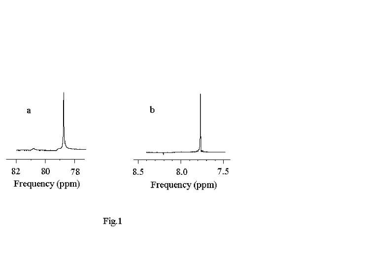
Figure 1:

2

Figure 2:

3

Figure 3: