Stokes operator squeezed continuous variable polarization states

Abstract

We investigate quantum correlations in continuous wave polarization squeezed laser light generated from one and two optical parametric amplifiers, respectively. A general expression of how Stokes operator variances decompose into two mode quadrature operator variances is given. Stokes parameter variance spectra for four different polarization squeezed states have been measured and compared with a coherent state. Our measurement results are visualized by three-dimensional Stokes operator noise volumes mapped on the quantum Poincaré sphere. We quantitatively compare the channel capacity of the different continuous variable polarization states for communication protocols. It is shown that squeezed polarization states provide 33% higher channel capacities than the optimum coherent beam protocol.

I introduction

The quantum properties of the polarization of continuous wave light are of increasing interest since they offer new opportunities for communicating quantum information with light and for transferring quantum information from atoms to photons and vice versa. In the single photon regime the quantum polarization states have been vigorously studied, theoretically and experimentally, with investigations of fundamental problems of quantum mechanics, such as Bell’s inequality Bell-theo ; Bell-exp , and of potential applications such as quantum cryptography QCr-theo ; QCr-exp . In comparison, continuous variable quantum polarization states have received little attention. Recently however, due to their apparent usefulness to quantum communication schemes, interest in them has been growing and a number of theoretical papers have been published APu89 –KLLRS02 .

Continuous variable quantum polarization states can be carried by a bright laser beam, providing high bandwidth capabilities and therefore faster signal transfer rates than single photon systems. In addition, several proposals have been made for quantum networks that consist of spatially separated nodes of atoms whose spin states enable the storage and processing of information, connected by optical quantum communication channels DiVin95 –KuzPolzik00 . Mapping of quantum states from photonic to atomic media is a crucial element in these networks. For continuous variable polarization states this mapping has been experimentally demonstrated HSSP99 . Even one of the fundamental phenomena of quantum physics, entanglement, has been realized for the macroscopic spin states of two gas samples JKP01 . Very recently entanglement was experimentally demonstrated for optical continuous variable polarization states for the first time BTSL02 .

Several methods for generating continuous variable polarization squeezed states have been proposed, most using nonlinearity provided by Kerr-like media and optical solitons KCh96 ; AAC98 ; KLLRS02 . The two experimental demonstrations previous to our work reported here and in BSBL02 , however, were achieved by combining a dim quadrature squeezed beam with a bright coherent beam on a polarizing beam splitter HSSP99 ; GSYL87 . In both cases only the properties of the state relevant to the experimental outcome were characterized. The full characterization of a continuous variable polarization state requires measurements of the fluctuations in both the orientation, and the length of the Stokes vector on a Poincaré sphere.

In this paper we present the complete experimental characterization of the Stokes vector fluctuations for four different quantum polarization states. We make use of ideas recently published by Korolkova et al. KLLRS02 . Their concept of squeezing more than one Stokes operator of a laser beam and a simple scheme to measure the Stokes operator variances are realized. Our results given in BSBL02 are extended and discussed in more detail. Experimental data from polarization squeezed states generated from a single quadrature squeezed beam and from two quadrature squeezed beams are compared.

The outline of this paper is as follows. We present a description of the theory involved in our experiments. Since polarization states can be decomposed into two mode quadrature states a general link between Stokes operator variances and quadrature variances is given. In the experimental section we characterize the polarization fluctuations of a single amplitude squeezed beam from an optical parametric amplifier (OPA). It can be seen that only the fluctuations of the Stokes vector length are below that of a coherent beam (ie. squeezed). Grangier et al. GSYL87 and Hald et al. HSSP99 converted this to squeezing of the Stokes vector orientation by combining the quadrature squeezed beam with a much brighter coherent beam on a polarizing beam splitter. We experimentally generate this situation and indeed show that the Stokes vector orientation is squeezed. This result is compared with measurements on polarization states generated from two quadrature squeezed beams. Two bright amplitude or phase squeezed beams from two independent OPAs are overlapped on a polarizing beam splitter KLLRS02 ; BSBL02 demonstrating “pancake-like” and “cigar-like” uncertainty volumes on the Poincaré sphere for phase and amplitude squeezed input beams, respectively. Both the orientation and the length of the Stokes vector were squeezed for the “cigar-like” uncertainty volume. In the final section several schemes for encoding information on continuous variable polarization states of light are discussed. The conventional fiber-optic communication protocol is compared with optimized coherent beam and squeezed beam protocols. We show that the channel capacity of the “cigar-like” polarization squeezed states exceeds the channel capacity of all the other states.

II Theoretical background

.

Figure 1: Diagram of a) classical and b) quantum Stokes vectors mapped on a Poincaré sphere; the ball at the end of the quantum vector visualizes the quantum noise in $\rm\hat{S}_{1}$, $\rm\hat{S}_{2}$, and $\rm\hat{S}_{3}$; and the non-zero quantum sphere thickness visualizes the quantum noise in $\rm\hat{S}_{0}$.

The polarization state of a light beam in classical optics can be visualized as a Stokes vector on a Poincaré sphere (Fig. 1) and is determined by the four Stokes parameters Sto52 : $S_{0}$ represents the average beam intensity whereas $S_{1}$, $S_{2}$, and $S_{3}$ characterize its polarization and form a Cartesian axes system. If the Stokes vector points in the direction of $S_{1}$, $S_{2}$, or $S_{3}$ the polarized part of the beam is horizontally, linearly at 45^∘, or right-circularly polarized, respectively. Two beams are said to be opposite in polarization and do not interfere if their Stokes vectors point in opposite directions. The quantity $\,S=(S_{1}^{2}+S_{2}^{2}+S_{3}^{2})^{1/2}\,$ is the radius of the classical Poincaré sphere and describes the average intensity of the polarized part of the radiation. The fraction $\,S/S_{0}\,$ ($\,0\!<\!S/S_{0}\!<\!1\,$) is called the degree of polarization. For quasi-monochromatic laser light which is almost completely polarized $S_{0}$ is a redundant parameter, completely determined by the other three parameters ($S_{0}\!=\!S$ in classical optics). All four Stokes parameters are accessible from the simple experiments shown in Fig. 2.

Figure 2: Apparatus required to measure each of the Stokes parameters. PBS: polarizing beam splitter, $\lambda/2$ and $\lambda/4$: half- and quarter-wave plates respectively, the plus and minus signs imply that an electrical sum or difference has been taken.

An equivalent representation of polarization states of light is given by the 4 elements of the coherence matrix (Jones matrix). The relations between these elements and the Stokes parameters can be found in WolfMandel . In contrast to the coherence matrix elements the Stokes parameters are observables and therefore can be associated with Hermitian operators. Following JauchRohrlich76 and Robson74 we define the quantum-mechanical analogue of the classical Stokes parameters for pure states in the commonly used notation:

$$\hat{S}_{0}\! = \hat{a}_{H}^{\dagger}\hat{a}_{H}+\hat{a}_{V}^{\dagger}\hat{a}_{V}~{},\hskip 28.45274pt$$

$$\hat{S}_{1}\! = \hat{a}_{H}^{\dagger}\hat{a}_{H}-\hat{a}_{V}^{\dagger}\hat{a}_{V}~{},\hskip 28.45274pt$$ (1)

$$\hat{S}_{2}\! = \hat{a}_{H}^{\dagger}\hat{a}_{V}e^{i\theta}\!+\hat{a}_{V}^{\dagger}\hat{a}_{H}e^{-i\theta}~{},$$

$$\hat{S}_{3}\! = i\hat{a}_{V}^{\dagger}\hat{a}_{H}e^{-i\theta}\!-i\hat{a}_{H}^{\dagger}\hat{a}_{V}e^{i\theta}~{},$$

where the subscripts $H$ and $V$ label the horizontal and vertical polarization modes respectively, $\theta$ is the phase shift between these modes, and the $\hat{a}_{H,V}$ and $\hat{a}_{H,V}^{\dagger}$ are annihilation and creation operators for the electro-magnetic field in frequency space footnote1 .

The commutation relations of the annihilation and creation operators

$$[\hat{a}_{k},\hat{a}_{l}^{\dagger}]=\delta_{kl}~{},\hskip 11.38109pt\mbox{with}\hskip 11.38109ptk,l\in\{H,V\}~{},$$ (2)

directly result in Stokes operator commutation relations,

$$[\hat{S}_{1},\hat{S}_{2}]=2i\hat{S}_{3}~{},\hskip 5.69054pt[\hat{S}_{2},\hat{S}_{3}]=2i\hat{S}_{1}~{},\hskip 5.69054pt[\hat{S}_{3},\hat{S}_{1}]=2i\hat{S}_{2}~{}\,.$$ (3)

Apart from a normalization factor, these relations are identical to the commutation relations of the Pauli spin matrices. In fact the three Stokes parameters in Eq. (3) and the three Pauli spin matrices both generate the special unitary group of symmetry transformations SU(2) of Lie algebra Kaku93 . Since this group obeys the same algebra as the three-dimensional rotation group, distances in three dimensions are invariant. Accordingly the operator $\hat{S}_{0}$ is also invariant and commutes with the other three Stokes operators ($\,[\hat{S}_{0},\hat{S}_{j}]=0,\;\mbox{with}\;j=1,2,3$). The non-commutability of the Stokes operators $\hat{S}_{1}$, $\hat{S}_{2}$ and $\hat{S}_{3}$ precludes the simultaneous exact measurement of their physical quantities. As a direct consequence of Eq.(3) the Stokes operator mean values $\,\langle\hat{S}_{j}\rangle\,$ and their variances $\,V_{j}=\langle\hat{S}_{j}^{2}\rangle\!-\!\langle\hat{S}_{j}\rangle^{2}\,$ are restricted by the uncertainty relations JauchRohrlich76

$$V_{1}V_{2}\geq|\langle\hat{S}_{3}\rangle|^{2}~{},~{}V_{2}V_{3}\geq|\langle\hat{S}_{1}\rangle|^{2}~{},~{}V_{3}V_{1}\geq|\langle\hat{S}_{2}\rangle|^{2}~{}.$$ (4)

In general this results in non-zero variances in the individual Stokes parameters as well as in the radius of the Poincaré sphere (see Fig. 1b)). The quantum noise in the Stokes parameters even effects the definitions of the degree of polarization APu89 ; AAC98 and the Poincaré sphere radius. It can be shown from Eqs. (II) and (2) that the quantum Poincaré sphere radius is different from its classical analogue, $\,\langle\hat{S}\rangle=\langle\hat{S}_{0}^{2}+2\hat{S}_{0}\rangle^{1/2}\,$.

Recently it has been shown that the Stokes operator variances may be obtained from the frequency spectrum of the electrical output currents of the setups shown in Fig. 2 KLLRS02 . To calculate the Stokes operator variances we use the linearized formalism here. The creation and annihilation operators are expressed as sums of real classical amplitudes $\alpha_{H,V}$ and quantum noise operators $\delta\hat{a}_{H,V}$ WallsMilburn

$$\hat{a}_{H,V}=\alpha_{H,V}+\delta\hat{a}_{H,V}~{}.$$ (5)

The operators in Eq.(5) are non-hermitian and therefore non-physical. To express the Stokes operators of Eq. (II) in terms of hermitian operators we define the generalized quadrature quantum noise operators $\delta\hat{X}_{H,V}(\xi)$

$$\delta\hat{X}_{H,V}(\xi)= \delta\hat{a}^{\dagger}_{H,V}e^{i\xi}+\delta\hat{a}_{H,V}e^{-i\xi}~{},\hskip 17.07164pt$$ (6)

$$\delta\hat{X}_{H,V}(\xi\!=\!0)= \delta\hat{X}^{+}_{H,V}=\delta\hat{a}^{\dagger}_{H,V}+\delta\hat{a}_{H,V}~{},\hskip 8.53581pt$$ (7)

$$\delta\hat{X}_{H,V}(\xi\!=\!\pi/2)= \delta\hat{X}^{-}_{H,V}=i(\delta\hat{a}^{\dagger}_{H,V}-\delta\hat{a}_{H,V})~{}.$$ (8)

$\xi$ is the phase of the quantum mechanical oscillator and $\delta\hat{X}_{H,V}^{+}$ and $\delta\hat{X}_{H,V}^{-}$ are the amplitude quadrature noise operator and the phase quadrature noise operator respectively.

If the variances of the noise operators are much smaller than the coherent amplitudes then a first order approximation of the noise operators is appropriate. This yields the Stokes operator mean values

$$\langle\hat{S}_{0}\rangle = \alpha_{H}^{2}+\alpha_{V}^{2}=\langle\hat{n}\rangle~{},\hskip 5.69054pt$$

$$\langle\hat{S}_{1}\rangle = \alpha_{H}^{2}-\alpha_{V}^{2}~{},\hskip 32.72066pt$$ (9)

$$\langle\hat{S}_{2}\rangle = 2\alpha_{H}\alpha_{V}\,\mbox{cos}\theta~{},$$

$$\langle\hat{S}_{3}\rangle = 2\alpha_{H}\alpha_{V}\,\mbox{sin}\theta~{},$$

These expressions are identical to the Stokes parameters in classical optics. Here $\,\langle\hat{n}\rangle\,$ is the expectation value of the photon number operator. For a coherent beam the expectation value and variance of $\hat{n}$ have the same magnitude, this magnitude equals the conventional shot-noise level. The variances of the Stokes parameters are given by

$$\,V_{0}= \!\alpha_{H}^{2}\langle(\delta\hat{X}_{H}^{+})^{2}\rangle\!+\alpha_{V}^{2}\langle(\delta\hat{X}_{V}^{+})^{2}\rangle+2\alpha_{H}\alpha_{V}\langle\delta\hat{X}_{H}^{+}\delta\hat{X}_{V}^{+}\rangle,\hskip 14.22636pt$$

$$\,V_{1}= \!\alpha_{H}^{2}\langle(\delta\hat{X}_{H}^{+})^{2}\rangle\!+\alpha_{V}^{2}\langle(\delta\hat{X}_{V}^{+})^{2}\rangle-2\alpha_{H}\alpha_{V}\langle\delta\hat{X}_{H}^{+}\delta\hat{X}_{V}^{+}\rangle,\hskip 14.22636pt$$

$$V_{2}(\theta) \!\!=\alpha_{H}^{2}\langle(\delta\hat{X}_{V}(-\theta))^{2}\rangle\!+\alpha_{V}^{2}\langle(\delta\hat{X}_{H}(\theta))^{2}\rangle\;,\hskip 36.98857pt$$

$$+2\alpha_{H}\alpha_{V}\langle\delta\hat{X}_{V}(-\theta)\delta\hat{X}_{H}(\theta)\rangle\;,\hskip 45.5244pt$$

$$V_{3}(\theta) \!=V_{2}(\theta\!-\!\frac{\pi}{2})\;.\hskip 153.64487pt$$

It can be seen from Eqs.(II) that the variances of Stokes operators can be expressed in terms of the variances of quadrature operators of two modes. The polarization squeezed state can then be defined in a straight forward manner. The variances of the noise operators in the above equation are normalized to one for a coherent beam. Therefore the variances of the Stokes parameters of a coherent beam are all equal to the shot-noise of the beam. For this reason a Stokes parameter is said to be squeezed if its variance falls below the shot-noise of an equal power coherent beam. Although the decomposition to the $H,V$-polarization axis of Eqs. (II) is independent of the actual procedure of generating a polarization squeezed beam, it becomes clear that two overlapped quadrature squeezed beams can produce a single polarization squeezed beam. If two beams in the horizontal and vertical polarization mode having uncorrelated quantum noise are used Eqs. (II) can be rewritten as

$$V_{0}\,=\!\! \!\!\!\!V_{1}\,=\alpha_{H}^{2}\langle(\delta\hat{X}_{H}^{+})^{2}\rangle\!+\!\alpha_{V}^{2}\langle(\delta\hat{X}_{V}^{+})^{2}\rangle~{},\hskip 2.84526pt$$

$$V_{2}(\theta)=\!\! \!\!\!\mbox{cos}^{2}\theta\left(\alpha_{V}^{2}\langle(\delta\hat{X}_{H}^{+})^{2}\rangle\!+\!\alpha_{H}^{2}\langle(\delta\hat{X}_{V}^{+})^{2}\rangle\right)\hskip 8.53581pt$$ (11)

$$+\mbox{sin}^{2}\theta\left(\alpha_{V}^{2}\langle(\delta\hat{X}_{H}^{-})^{2}\rangle\!+\!\alpha_{H}^{2}\langle(\delta\hat{X}_{V}^{-})^{2}\rangle\right),\hskip 14.22636pt$$

$$V_{3}(\theta)=\!\! \!V_{2}(\theta\!-\!\frac{\pi}{2})~{}.\hskip 119.50157pt$$

Here we choose the amplitude and the phase quadrature noise operators to express the variances. This corresponds to our actual experimental setup where either amplitude or the phase quadratures were squeezed. It can be seen from Eqs.(II) that in a polarization squeezed beam generated from two amplitude squeezed beams $\hat{S}_{0}$ and two additional Stokes parameters can in theory be perfectly squeezed while the fourth is anti-squeezed if specific angles of $\,\theta\!=\!0$ or $\,\theta\!=\!\pi/2\,$ are used. Utilizing only one squeezed beam it is not possible to simultaneously squeeze any two of $\hat{S}_{1}$, $\hat{S}_{2}$, and $\hat{S}_{3}$ to quieter than 3 dB below shot-noise ($V_{i}\!+\!V_{j}\!\geq\!\langle\hat{n}\rangle$, with $i,j\in\{1,2,3;i\!\not=\!j\}$).

III Experiment

Prior to our work presented here and in BSBL02 , polarization squeezed states were generated by combining a strong coherent beam with a single weak amplitude squeezed beam GSYL87 ; HSSP99 . In both of those experiments the variance of only one Stokes parameter was determined, and therefore the polarization state was not fully characterized. In this paper we experimentally characterize the mean and variance of all four Stokes operators for these states. We extend the work to polarization squeezed states produced from two amplitude/phase squeezed beams. Fig. 3 shows our experimental setup.

Figure 3: Schematic of the polarization squeezing experiment. MC: mode cleaner, BS: beam splitter, DC: dichroic beam splitter, $\lambda/2$: half-wave plate, $\phi_{\rm{SH}}$: phase shift between 532 nm and 1064 nm light at the OPAs, $\theta$: phase shift between quadrature squeezed beams, PBS: polarizing beam splitter, H: horizontal polarization mode, V: vertical polarization mode.

III.1 Generation of quadrature squeezed light

We produced the two quadrature squeezed beams required for this experiment in a pair of OPAs. Each OPA was an optical resonator consisting of a hemilithic MgO:LiNbO₃ crystal and an output coupler. The reflectivities of the output coupler were 96% and 6% for the fundamental (1064 nm) and the second harmonic (532 nm) laser modes, respectively. Each OPA was pumped with single-mode 532 nm light generated by a 1.5 W Nd:YAG non-planar ring laser and frequency doubled in a second harmonic generator (SHG). The SHG was of identical structure to the OPAs but with 92% reflectivity at 1064 nm. The OPAs were seeded with 1064 nm light after spectral filtering in a modecleaner. The refractive indices of the MgO:LiNbO₃ crystals in each resonator was modulated with an RF field, this provided error signals on the reflected seed power that were used to lock their lengths. The modulation also resulted in a phase modulation on the output beams from the SHG and each OPA. The coherent amplitude of each OPAs output was a deamplified/amplified version of the seed coherent amplitude; the level of amplification was dependent on the phase difference between pump and seed ($\phi_{\rm{SH}}$). Therefore the second harmonic pump phase modulation resulted in a modulation of the amplification of the OPAs. Error signals could be extracted from this effect, enabling the relative phase between pump and seed to be locked. Locking to deamplification or amplification provided an amplitude or phase squeezed output, respectively. Typical measured variance spectra of the two locked quadrature squeezed beams are shown in Fig. 4. Since the squeezed states were carried by bright laser beams of approximately 1 mW, the noise reduction was degraded at lower frequencies due to the laser relaxation oscillation. At higher frequencies the squeezed spectrum was limited by the bandwidth of the OPAs.

Figure 4: Typical measured variance spectra of the two locked bright quadrature squeezed beams.

Past experiments requiring two quadrature squeezed beams commonly used a single ring resonator with two outputs Ou ; with two independent OPAs the necessary intracavity pump power is halved, this reduces the degradation of squeezing due to green-induced infrared absorption (GRIIRA) Furukawa .

III.2 Measuring the Stokes operators

Instantaneous values of the Stokes operators of all polarization states analyzed in this paper were obtained with the apparatus shown in Fig. 2. The uncertainty relations of Eqs. 4 dictate that $\hat{S}_{1}$, $\hat{S}_{2}$, and $\hat{S}_{3}$ cannot be measured simultaneously. The beam under interrogation was split on a polarizing beam splitter and the two outputs were detected on a pair of high quantum efficiency photodiodes with 30 MHz bandwidth; the resulting photocurrents were added and subtracted to yield photocurrents containing the instantaneous values of $\hat{S}_{0}$ and $\hat{S}_{1}$. To measure $\hat{S}_{2}$ the polarization of the beam was rotated by 45^∘ with a half-wave plate before the polarizing beam splitter and the detected photocurrents were subtracted. To measure $\hat{S}_{3}$ the polarization of the beam was again rotated by 45^∘ with a half-wave plate and a quarter-wave plate was introduced before the polarizing beam splitter such that a horizontally polarized input beam became right-circularly polarized. Again the detected photocurrents were subtracted. The expectation value of each Stokes operator was equal to the DC output of the detection device and the variance was obtained by passing the output photocurrent into a Hewlett-Packard E4405B spectrum analyzer. Every polarization state interrogated in this work had a total power $\langle\hat{S}_{0}\rangle$ of roughly 2 mW.

An accurate shot-noise level was required to determine whether any given Stokes operator was squeezed. This was measured by operating a single OPA without the second harmonic pump. The seed power was adjusted so that the output power was equal to that of the beam being interrogated. In this configuration the detection setup for $\hat{S}_{2}$ (see Fig. 2c)) functions exactly as a homodyne detector measuring vacuum noise scaled by the OPA output power, the variance of which is the shot-noise. Throughout each experimental run the power was monitored and was always within 2% of the power of the coherent calibration beam. This led to a conservative error in our frequency spectra of $\pm$0.05 dB.

The Stokes operator variances reported in this paper were taken over the range from 3 to 10 MHz. The darknoise of the detection apparatus was always more than 4 dB below the measured traces and was taken into account. Each displayed trace is the average of three measurement results normalized to the shot-noise and smoothed over the resolution bandwidth of the spectrum analyzer which was set to 300 kHz. The video bandwidth of the spectrum analyzer was set to 300 Hz.

As is the case for all continuous variable quantum optical experiments, the efficiency of the Stokes operator measurements was critical. The overall detection efficiency of the interrogated beams was 76%. The loss came primarily from three sources: loss in escape from the OPAs (14%), detector inefficiency (7%), and loss in optics (5%). In the experiment where a squeezed beam was overlapped with a coherent beam additional loss was incurred due to poor mode-matching between the beams and the detection efficiency was 71%. Depolarizing effects are thought to be another significant source of loss for some polarization squeezing proposals APu89 . In our scheme the non-linear processes (OPAs) are divorced from the polarization manipulation (wave plates and polarizing beam splitters), and depolarizing effects are insignificant.

III.3 Quantum polarization states from a single squeezed beam

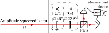
Figure 5: Apparatus used to produce and analyze a single amplitude squeezed beam. Optics in a) and b) were included to measure the variance and the expectation value of $\hat{S}_{2}$ and $\hat{S}_{3}$, respectively.

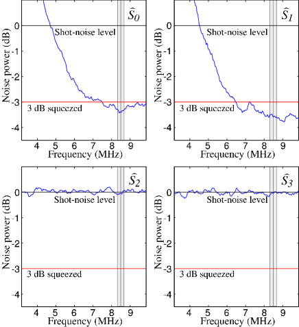
Figure 6: Measured variance spectra of quantum noise on $\hat{S}_{0}$, $\hat{S}_{1}$, $\hat{S}_{2}$, and $\hat{S}_{3}$ for a single bright amplitude squeezed beam; normalized to shot-noise. The shaded region was used to construct the Poincaré sphere representation in Fig. 12 b).

We first characterize the polarization state of a single bright amplitude squeezed beam provided by one of our OPAs, as shown in Fig. 5. The squeezed beam was horizontally polarized, resulting in Stokes operator expectation values of $\langle\hat{S}_{0}\rangle\!=\!\langle\hat{S}_{1}\rangle\!=\!|\alpha_{H}|^{2}$ and $\langle\hat{S}_{2}\rangle\!=\!\langle\hat{S}_{3}\rangle\!=\!0$. The variance spectra of the operators were measured and are displayed in Fig. 6. $\hat{S}_{0}$ and $\hat{S}_{1}$ were squeezed since the horizontally polarized amplitude squeezed beam hit only one detector in this detector setup. For the measurements of $\hat{S}_{2}$ and $\hat{S}_{3}$ the beam intensity was divided equally between the two detectors. The electronic subtraction yielded vacuum noise scaled by the beam intensity, thus both variance measurements were at the shot noise level. It is apparent from these measurements that only the length of the Stokes vector is well determined; the orientation is just as uncertain as it would be for a coherent state.

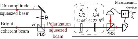
Figure 7: Apparatus used to produce and analyze the polarization squeezed beam produced by overlapping a dim quadrature squeezed beam with a bright coherent beam. Optics in a) and b) were included to measure the variance and the expectation value of $\hat{S}_{2}$ and $\hat{S}_{3}$, respectively.

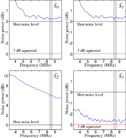
Figure 8: Measured variance spectra of quantum noise on $\hat{S}_{0}$, $\hat{S}_{1}$, $\hat{S}_{2}$, and $\hat{S}_{3}$ for a vacuum amplitude squeezed and a bright coherent input beams; normalized to shot-noise. The shaded region was used to construct the Poincaré sphere representation in Fig. 12 c).

To obtain squeezing of the orientation of the Stokes vector Grangier et al. GSYL87 and Hald et al. HSSP99 overlapped a dim quadrature squeezed beam with a bright orthogonally polarized coherent beam. We consider this situation next (as shown in Fig. 8). Since two beams are now involved, the relative phase $\theta$ becomes important. A DC and an RF error-signal, both dependant on $\theta$, were extracted from the Stokes operator measurement device. Together, these error signals allowed us to lock $\theta$ to either 0 or $\pi/2$ rads in all of the following experiments. We mixed a bright horizontally polarized coherent beam with a dim vertically polarized amplitude squeezed beam. Since the horizontally polarized beam was much more intense than the vertically polarized beam, the Stokes operator expectation values became $\langle\hat{S}_{0}\rangle\!\approx\!\langle\hat{S}_{1}\rangle\!\approx\!|\alpha_{H}|^{2}$ and $\langle\hat{S}_{2}\rangle\!\approx\!\langle\hat{S}_{3}\rangle\!=\!0$. The Stokes operator variances obtained for this polarization state are shown in Fig. 8, here $\hat{S}_{2}$ is anti-squeezed and $\hat{S}_{3}$ is squeezed. The variances of $\hat{S}_{0}$ and $\hat{S}_{1}$ were slightly above the shot-noise level because of residual noise from our laser resonant relaxation oscillation. The experiment carried out with $\theta$ locked to 0 rads is not shown, in this case the measured variances of $\hat{S}_{2}$ and $\hat{S}_{3}$ were swapped. In fact the Stokes vector was still pointing along $\hat{S}_{1}$ but the quantum noise was rotated on the Poincaré sphere (see Fig. 13b).

III.4 Quantum polarization states from two quadrature squeezed beams

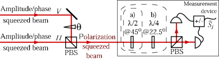
Figure 9: Apparatus used to produce and analyze the beam produced by combining two quadrature squeezed beams. Optics in a) and b) were included to measure the variance and the expectation value of $\hat{S}_{2}$ and $\hat{S}_{3}$, respectively.

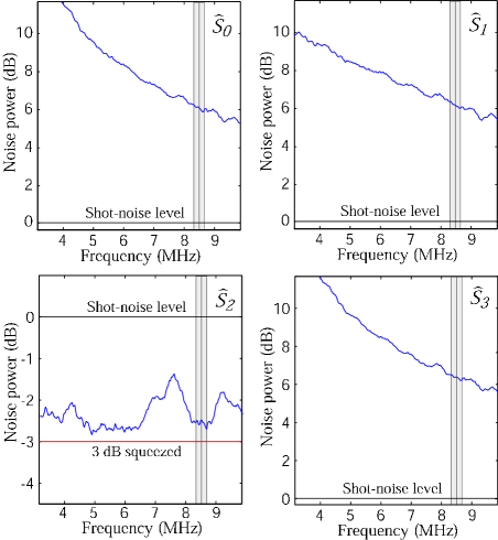
Figure 10: Measured variance spectra of quantum noise on $\hat{S}_{0}$, $\hat{S}_{1}$, $\hat{S}_{2}$, and $\hat{S}_{3}$ for two locked phase squeezed input beams; normalized to shot-noise. The shaded region was used to construct the Poincaré sphere representation in Fig. 12 d).

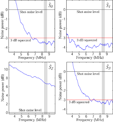
Figure 11: Measured variance spectra of quantum noise on $\hat{S}_{0}$, $\hat{S}_{1}$, $\hat{S}_{2}$, and $\hat{S}_{3}$ for two locked amplitude squeezed input beams; normalized to shot-noise. The shaded region was used to construct the Poincaré sphere representation in Fig. 12 e).

The two experiments described in Section III.3 demonstrated how it is possible to squeeze the length and orientation of the Stokes vector. In this section we demonstrate that it is possible to do both simultaneously. The two quadrature squeezed beams produced in our OPAs were combined with orthogonal polarization on a polarizing beam splitter KLLRS02 as shown in Fig. 9. This produced an output beam with Stokes parameter variances as given by Eqs. (II). Both input beams had equal power ($\alpha_{H}\!=\!\alpha_{V}\!=\!\alpha/\sqrt{2}$) and both were squeezed in the same quadrature. The Stokes parameters and their variances were again determined as shown in Fig. 2. The relative phase between the quadrature squeezed input beams $\theta$ was locked to $\pi/2$ rads producing a right-circularly polarized beam with Stokes parameter means of $\langle\hat{S}_{1}\rangle\!=\!\langle\hat{S}_{2}\rangle\!=\!0$ and $\langle\hat{S}_{0}\rangle\!=\!\langle\hat{S}_{3}\rangle\!=\!|\alpha|^{2}$.

First both OPA pump beams were phase locked to amplification, this produced two phase squeezed beams. Fig. 10 shows the measurement results obtained; $\hat{S}_{0}$, $\hat{S}_{1}$ and $\hat{S}_{3}$ were all anti-squeezed and $\hat{S}_{2}$ was squeezed throughout the range of the measurement. The optimum noise reduction of $\hat{S}_{2}$ was 2.8 dB below shot-noise and was observed at 4.8 MHz. Our OPAs are particularly sensitive to phase noise coupling in from the MgO:LiNbO₃ crystals. We attribute the structure in the frequency spectra of $\hat{S}_{2}$ and the poorer squeezed observed here, to this. Apart from this structure, these results are very similar to those produced by a single squeezed beam and a coherent beam; the orientation of the Stokes vector is squeezed. However, here the uncertainty in the length of the Stokes vector is greater than for a coherent state so the polarization state, although produced from two quadrature squeezed beams, is actually less certain.

Fig. 11 shows the measurement results obtained with the OPAs locked to deamplification. Therefore both OPAs provided amplitude squeezed beams. Again we interrogated the combined beams and found $\hat{S}_{0}$, $\hat{S}_{1}$ and $\hat{S}_{3}$ all to be squeezed from 4.5 MHz to the limit of our measurement, 10 MHz. $\hat{S}_{2}$ was anti-squeezed throughout the range of the measurement. Between 7.2 MHz and 9.6 MHz $\hat{S}_{0}$, $\hat{S}_{1}$ and $\hat{S}_{3}$ were all more than 3 dB below shot-noise. The squeezing of $\hat{S}_{0}$ and $\hat{S}_{3}$ was degraded at low frequency due our lasers resonant relaxation oscillation. Since this noise was correlated it canceled in the variance of $\hat{S}_{1}$. The maximum squeezing of $\hat{S}_{0}$ and $\hat{S}_{2}$ was 3.8 dB and 3.5 dB respectively and was observed at 9.3 MHz. The maximum squeezing of $\hat{S}_{1}$ was 4.3 dB at 5.7 MHz. The repetitive structure at 4, 5, 6, 7, 8 and 9 MHz was caused by electrical pick-up in our SHG resonator emitted from a separate experiment operating in the laboratory. In this case both the orientation and the length of the Stokes vector were squeezed.

Finally we point out that the variances of $\hat{S}_{1}$ in Figs. 8, 10 and 11 were all squeezed at frequencies down to 3 MHz and even below, whereas Fig. 4 shows a clear degradation below 4 MHz. This improved performance is due to electrical noise cancellation of correlated laser relaxation oscillation noise. This noise is effectively reduced by taking the difference of the two photo currents in our detector setup to measure $V_{1}$.

IV Visualization of quantum correlations in continuous variable polarization states

Figure 12: Measured quantum polarization noise at 8.5 MHz from different combinations of input beams. a) single coherent beam, b) coherent beam and squeezed vacuum, c) bright squeezed beam, d) two phase squeezed beams and e) two amplitude squeezed beams. The surface of the ellipsoids defines the standard deviation of the noise normalized to shot-noise ($\sigma_{S_{i}}\!=\!\sqrt{V_{i}}$). $\hat{S}_{/\!/}$ denotes the Stokes operator along the Stokes vector.

Figure 13: Visualization of measured quantum noise and measured Stokes vectors of four polarization states mapped onto the Poincaré sphere. The states were generated from a) two bright amplitude squeezed inputs and b) a bright coherent beam and a amplitude squeezed vacuum. The rotation in a) and also in b) was achieved by a $\,\theta=\pi/2$ phase shift or an additionally introduced $\lambda/4$ wave plate.

In this section measured quantum correlations in polarization states at 8.5 MHz are visualized. Based on the theoretical formalism in Section II continuous variable polarization states can be characterized by the measurement of Stokes operator expectation values and variances using the setup shown in Fig. 2. Our noise measurement results at 8.5 MHz on five different states are summarized in Fig. 12. The noise characteristics of the Stokes parameters are mapped onto the coordinate system of the Poincaré sphere, assuming Gaussian noise statistics. Given this assumption, the standard deviation contour-surfaces shown here provide an accurate representation of the states three-dimensional noise distribution. The quantum polarization noise of a coherent state forms a sphere of noise as portrayed in Fig. 12 a). The noise volumes b) to e) visualizes the measurements on a single bright amplitude squeezed beam, on the combination of a vacuum amplitude squeezed beam and a bright coherent beam, on two locked phase squeezed input beams and on two locked amplitude squeezed beams, respectively. In all cases the Stokes operator noise volume describes the end position of the Stokes vector pointing upwards. In b) and c) the Stokes vectors are parallel to the direction of $S_{1}$, in d) and e) parallel to the direction of $S_{3}$, since we used horizontally and right-circularly polarized light, respectively. However, there was no fundamental bias in the orientation of the quantum Stokes vector in our experiment. By varying the angle of an additional half-wave plate in the polarization squeezed beam or by varying $\theta$ any orientation may be achieved. In fact, as mentioned earlier our experiments were also carried out with $\theta$ locked to 0 rads. This had the effect of rotating the Stokes vector and its quantum noise by $\pi/2$ around $\hat{S}_{1}$. Nearly identical results were obtained but on alternative Stokes parameters. Fig. 13 a) shows Poincaré sphere representations of this rotation for the polarization states produced by two amplitude squeezed beams. In Fig. 13 b) the combination of a amplitude squeezed vacuum and a bright coherent beam exemplifies that different orientations of the noise volume can be generated using appropriate combination of waveplates.

V Channel Capacity of Polarization Squeezed Beams

The reduced level of fluctuations in polarization squeezed light can be used to improve the channel capacity of communication protocols. Let us consider information encoded on the sidebands of a bandwidth limited single spatial mode laser beam. We assume that only direct detection is employed, or in other words, that phase sensitive techniques such as homodyne measurement are not available. This is not an artificial constraint since phase sensitive techniques are technically difficult to implement and are rarely utilized in conventional optical communications systems.

An upper bound to the amount of information that can be carried by a bandwidth limited additive white Gaussian noise channel is given by the Shannon capacity C shan in bits per dimension

$$C={1\over 2}\log_{2}(1+R)~{}.$$ (12)

$R$ is the signal to noise ratio of the channel and is given by the ratio of the spectral variance of the signal modulation $V_{s}$ and the noise spectral variance $V_{n}$

$$R=\frac{V_{s}}{V_{n}}~{}.$$ (13)

We wish to compare the channel capacities achieveable with pure coherent and squeezed states for a given average photon number in the sidebands $\bar{n}$ where $\bar{n}\!=\!\langle\delta\hat{a}_{H}^{\dagger}\delta\hat{a}_{H}\!+\!\delta\hat{a}_{V}^{\dagger}\delta\hat{a}_{V}\rangle$. Note that $\bar{n}$ takes into account both, the signal modulation and the squeezing. An overview of quantum noise limited channel capacities may be found in YHa86 and CDr94 .

First let us consider strategies which might be employed with a coherent light beam. In conventional optical communication systems the polarization degrees of freedom are ignored completely and information is encoded only on $\hat{S}_{0}$ as intensity fluctuations. Taking $\alpha_{V}\!=\!0$ the variance of the Stokes operator $\hat{S}_{0}$ is given by $V_{0}\!=\!\alpha_{H}^{2}(V_{s}+1)$ in accordance with Eq. (II). For this one-dimensional coherent channel $V_{n}\!=\!\langle|\delta X_{H}^{+}|^{2}\rangle\!=\!1$ and therefore $R\!=\!V_{s}$. For this arrangement it can be shown that the average photon number per bandwidth per second is $\bar{n}\!=\!\frac{1}{4}V_{s}$ providing a photon resource limited Shannon capacity of

$$C_{\rm coh}^{i}={1\over 2}\log_{2}(1+4\bar{n})~{},$$ (14)

as a function of $\bar{n}$. This is a non-optimal strategy however. Examining Eqs. (3) and (II) we see that it is possible to choose an arrangement for which two of the Stokes operators commute and so can be measured simultaneously. Indeed it is easy to show that such simultaneous measurements can be made using only linear optics and direct detection. In particular let us assume that $\alpha_{H}\!=\!\alpha_{V}$ such that $\hat{S}_{2}$ and $\hat{S}_{3}$ commute, and use $\hat{S}_{2}$ and $\hat{S}_{3}$ as two independent information channels. Then $\hat{S}_{2}\!=\!\hat{S}_{0}$ and the information in both dimensions can be simultaneously extracted by subtracting and adding the photocurrents of the same pair of detectors. Assuming equal signal to noise ratios $R_{2}\!=\!R_{3}$ we find that $V_{s2}\!=\!V_{s3}\!=\!2\bar{n}$, and the channel capacity may be written

$$C_{\rm coh}^{ii} = {1\over 2}\log_{2}(1+R_{2})+{1\over 2}\log_{2}(1+R_{3})$$ (15)

$$= \log_{2}({1+2\bar{n}})~{}.$$

This channel capacity is always greater than that of Eq. (14) and for large $\bar{n}$ is 100 % greater.

For sufficiently high $\bar{n}$ a further improvement in channel capacity can be achieved. Consider placing signals on all three Stokes operators. Because of the non-commutation of $\hat{S}_{1}$ with $\hat{S}_{2}$ and $\hat{S}_{3}$ it is not possible to read out all three signals without a measurement penalty. Suppose the receiver adopts the following strategy: divide the beam on a beamsplitter with transmitivity $\epsilon$ and then measure $\hat{S}_{1}$ on the reflected output and $\hat{S}_{2}$ and $\hat{S}_{3}$ on the other output. Division of the beam will reduce the measured signal to noise ratios due to the injection of quantum noise at the beamsplitter such as $R_{1}\!=\!(1-\epsilon)V_{s1}$, $R_{2}\!=\!\epsilon V_{s2}$ and $R_{3}\!=\!\epsilon V_{s3}$. We find that for large $\bar{n}$ an optimum is reached with $\epsilon\!=\!2/3$ and the signal photon number in each Stokes parameter being $\bar{n}_{1}\!=\!\bar{n}_{2}\!=\!\bar{n}_{3}\!=\!\bar{n}/3$. Hence the channel capacity is

$$C_{\rm coh}^{iii} = {1\over 2}\log_{2}(1\!+\!R_{1})+{1\over 2}\log_{2}(1\!+\!R_{2})+{1\over 2}\log_{2}(1\!+\!R_{3})$$ (16)

$$= {1\over 2}\log_{2}({1+{4\over 9}\bar{n}})+\log_{2}({1+{8\over 9}\bar{n}})~{}.$$

This capacity beats that of Eq. (15) for $\bar{n}\!>\!7.56$. In summery the optimum coherent channel capacity is given by Eq. (16) for average photon numbers $\bar{n}\!>\!7.56$ and by Eq. (15) for lower values, see Fig. 14 traces c) and d).

Now let us examine the effect of polarization squeezing on the channel capacity. Consider first the simple case of intensity modulation on a single squeezed beam, which is equivalent to using a squeezed beam in the first coherent case considered (case i). The channel capacity can be maximized by optimizing the fraction of photons which are introduced by squeezing the quantum noise and the residual fraction of photons which actually carries the signal. For large photon numbers we find a proportioning of 0.5. For an average photon number of 1 just 1/3 of that photon should be used to reduce the quantum noise. The maximum channel capacity for a one-dimensional squeezed channel is found to be

$$C_{\rm 1sqz}^{i} = \log_{2}({1+2\bar{n}})~{},$$ (17)

which was previously given in YHa86 . This capacity beats only the corresponding coherent state. It is as efficient as the two-dimensional coherent channel, but less efficient than the three-dimensional coherent one for large photon numbers.

Consider now a polarization squeezed beam which is produced from a minimum uncertainty squeezed beam and a coherent beam, as in Section III.3. Suppose, as in case ii, that $\hat{S}_{2}$ and $\hat{S}_{3}$ commute and arrange that $\hat{S}_{2}$ has fluctuations at the quantum noise level while $\hat{S}_{3}$ is optimally squeezed. Again signals are encoded on $\hat{S}_{2}$ and $\hat{S}_{3}$. The channel capacity can be maximized by adjusting the relative signal sizes on the two Stokes operators for fixed average photon number as a function of the squeezing. Here 1/3 of the photons is used to squeeze and 2/3 is split equally for the two dimensions. The resultant maximum channel capacity is

$$C_{\rm 1sqz}^{ii} = {3\over 2}\log_{2}({1+{4\over 3}\bar{n}})~{}.$$ (18)

This always beats all three coherent state cases considered here, but in the limit of large $\bar{n}$ the advantage is minimal since the scaling with photon number is the same as that of $C_{\rm coh}^{iii}$ in Eq. (16).

If the polarization squeezed beam is produced from two amplitude squeezed beams as in Section III.4 the enhancement becomes more significant. Suppose again that $\hat{S}_{2}$ and $\hat{S}_{3}$ commute but now that both are optimally squeezed. Again encoding on $\hat{S}_{2}$ and $\hat{S}_{3}$, and varying the signal strength as a function of squeezing to maximize the channel capacity for a given $\bar{n}$. The maximum is reached when the photons are used to squeeze the noise and transport information in equal shares. The channel capacity for this arrangement is given by

$$C_{\rm 2sqz}^{ii} = 2\log_{2}({1+\bar{n}})~{},$$ (19)

which for large $\bar{n}$ is 33% greater than both the optimum coherent scheme and the scheme using a single quadrature squeezed beam. No further improvement of the channel capacity can be obtained by encoding the information on three Stokes parameters, as in case iii. Optimization of the beam splitter reflectivity results in the already considered two-dimensional arrangement. This is not a surprising result since the third Stokes parameter is anti-squeezed. Fig. 14 summarizes our results.

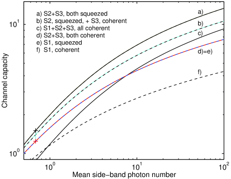
Figure 14: Calculated channel capacities for various continuous variable polarization states. The channels dimension and the channels quantum noise performance is varied. The cross in the upper curve marks the channel capacity which can be achieved using the polarization squeezed state in Fig. 11 and is compared with the optimum coherent state channel capacity (lower cross).

Finally we assess the channel capacities that could in principle be achieved using the polarization squeezed state generated in our experiment from two amplitude squeezed beams. The polarization squeezing achieved in Fig. 11 implies that, in the frequency range of 8 MHz to 10 MHz, 0.17 side-band photons per bandwidth and second were present in each of the two dimensions. This is an optimum quantum resource to transmit 0.68 side-band photons. Signals sufficiently high above detector dark noise would achieve a channel capacity that is around 21% greater than the ideal channel capacity achievable from a coherent beam with the same average side-band photon number (see crosses in Fig. 14).

VI Conclusion

The field of quantum communication and computation is receiving much attention. The continuous variable polarization states investigated here, are one of the most promising candidates for carrying the information in a quantum network. In this paper we have characterized the non classical properties of these states on the basis of the Stokes operators and their variances. Different classes of polarization squeezed states have been generated and experimentally characterized. We compared the coherent polarization state in Fig. 12a) with squeezed polarization states generated from a single amplitude squeezed beam Fig. 12c) and from two amplitude squeezed beams Fig. 12e), and proved that squeezing of better than 3 dB of three Stokes parameters ($\hat{S}_{0}$, $\hat{S}_{1}$, and $\hat{S}_{3}$) simultaneously is possible only in the latter case. We have theoretically analyzed the channel capacity for several communication protocols using continuous variable polarization states. For a given average photon number $\bar{n}$, we found the polarization state produced from two quadrature squeezed states can provide a 33% greater channel capacity than both the optimum coherent scheme and the scheme using a single quadrature squeezed beam.

We acknowledge the Alexander von Humboldt foundation for support of R. Schnabel; the Australian Research Council for financial support. This work is a part of EU QIPC Project, No. IST-1999-13071 (QUICOV).

References

- (1) J. S. Bell, Speakable and Unspeakable in Quantum Mechanics (Cambridge Univ. Press, Cambridge, 1988).
- (2) J. F. Clauser and A. Shimony, Rep. Prog. Phys. 41, 1881 (1978); A. Aspect, P. Grangier, and G. Roger, Phys. Rev. Lett. 49, 91 (1982).
- (3) S. Wiesner, Sigact News, 15, 78 (1983); C. H. Bennett and G. Brassard, Proceedings of IEEE International Conference on Computers, Systems and Signal Processing, Bangalore, India, December 1984, pp. 175-179; C. H. Bennett, Phys. Rev. Lett. 68, 3121 (1992); A. K. Ekert, Phys. Rev. Lett. 67, 661 (1991).
- (4) W. T. Buttler, R. J. Hughes, P. G. Kwiat, G. G. Luther, G. L. Morgan, J. E. Nordholt, C. G. Peterson, and C. M. Simons, Phys. Rev. A57, 2379 (1998); H. Zbinden, H. Bechmann-Pasquinacci, N. Gisin, and G. Ribordy, Appl. Phys. B 67, 743 (1998).
- (5) G. S. Agarwal and R. R. Puri, Phys. Rev. A40, 5179 (1989).
- (6) A. S. Chirkin, A. A. Orlov, and D. Y. Parashchuk, Quantum Electron. 23, 870 (1993).
- (7) V. P. Karasev and A. V. Masalov, Opt. Spectrosc., 74, 551 (1993).
- (8) N. V. Korolkova and A. S. Chirkin, Journal of Modern Optics 43, 869 (1996).
- (9) A. S. Chirkin, A. P. Alodjants, and S. M. Arakelian, Opt. Spectrosc., 82, 919 (1997).
- (10) P. A. Bushev, V. P. Karassiov, A. V. Masalov, and A. A. Putilin, Opt. Spectrosc., 91, 526 (2001).
- (11) A. P. Alodjants, S. M. Arakelian, and A. S. Chirkin, Appl. Phys. B 66, 53 (1998).
- (12) A. P. Alodjants, A. Y. Leksin, A. V. Prokhorov, and S. M. Arakelian, Laser Physics 12, 247 (2002).
- (13) T. C. Ralph, W. J. Munro, and R. E. S. Polkinghorne, Phys. Rev. Lett. 85, 2035 (2000).
- (14) N. Korolkova, G. Leuchs, R. Loudon, T. C. Ralph, and Ch. Silberhorn, Phys. Rev. A 65, 052306 (2002).
- (15) D. P. DiVincenzo, Science 270, 255 (1995).
- (16) J. I. Cirac and P. Zoller, Phys. Rev. Lett. 74, 4091 (1995).
- (17) A. Kuzmich and E. S. Polzik, Phys. Rev. Lett. 85, 5639 (2000).
- (18) J. Hald, J. L. Sørensen, C. Schori, and E. S. Polzik, Phys. Rev. Lett. 83 1319 (1999).
- (19) B. Julsgaard, A. Kozhekin, and E. S. Polzik, Nature, 413, 400 (2001).
- (20) W. P. Bowen, N. Treps, R. Schnabel, and P. K. Lam, Experimental demonstration of continuous variable polarization entanglement submitted for publication (2002), quant-ph/020617.
- (21) W. P. Bowen, R. Schnabel, H.-A. Bachor, and P. K. Lam, Phys. Rev. Lett. 88, 093601 (2002).
- (22) P. Grangier, R. E. Slusher, B. Yurke, and A. LaPorta, Phys. Rev. Lett. 59, 2153 (1987).
- (23) J. L. Sørensen, J. Hald, and E. S. Polzik, Phys. Rev. Lett. 80, 3487 (1998).
- (24) G. G. Stokes, Trans. Camb. Phil. Soc. 9, 399 (1852).
- (25) L. Mandel and E. Wolf, Optical Coherence and Quantum Optics, (Cambridge University Press, Cambridge, 1995).
- (26) J. M. Jauch and F. Rohrlich, The Theory of Photons and Electrons, 2nd ed., (Springer, Berlin, 1976).
- (27) B. A. Robson, The Theory of Polarization Phenomena, (Clarendon, Oxford, 1974).
- (28) Here we have excluded the phase difference from the mode operators to illustrate the link to our experiment more clearly.
- (29) See for example M. Kaku, Quantum Field Theory, (Oxford University Press, New York, 1993).
- (30) D. F. Walls and G. J. Milburn, Quantum Optics, (Springer, Berlin, 1995).
- (31) See for example Z. Y. Ou, S. F. Pereira, H. J. Kimble, and K. C. Peng, Phys. Rev. Lett. 68, 3663 (1992).
- (32) Y. Furukawa, K. Kitamura, A. Alexandrovski, R. K. Route, M. M. Fejer, and G. Foulon, Appl. Phys. Lett. 78, 1970 (2001).
- (33) C. E. Shannon, Bell System Tech. J. 27, 623 (1948).
- (34) Y. Yamamoto and H. A. Haus, Rev. Mod. Phys. 58, 1001 (1986).
- (35) C. M. Caves and P. D. Drummond, Rev. Mod. Phys. 66, 481 (1994).