Bounds and enhancements for the Hartman effect

Abstract

The time of passage of the transmitted wave packet in a tunneling collision of a quantum particle with a square potential barrier becomes independent of the barrier width in a range of barrier thickness. This is the Hartman effect, which has been frequently associated with “superluminality”. A fundamental limitation on the effect is set by non-relativistic “causality conditions”. We demonstrate first that the causality conditions impose more restrictive bounds on the negative time delays (time advancements) when no bound states are present. These restrictive bounds are in agreement with a naive, and generally false, causality argument based on the positivity of the “extrapolated phase time”, one of the quantities proposed to characterize the duration of the barrier’s traversal. Nevertheless, square wells may in fact lead to much larger advancements than square barriers. We point out that close to thresholds of new bound states the time advancement increases considerably, while, at the same time, the transmission probability is large, which facilitates the possible observation of the enhanced time advancement.

I Introduction

The Hartman effect occurs when the time of passage $t_{d}$ of the transmitted wave packet in a tunneling collision of a quantum particle with an opaque square barrier becomes essentially independent of the barrier width $d$ Hartman (1962); Fletcher (1985) ($t_{d}$ could be defined as the time of passage of the peak, or by means of some average of arrival or detection times as in Eq. (6) below). Since the velocity, when defined by comparing the instants of the incoming and outgoing peaks, may exceed arbitrarily large numbers, and there is a related effect for photons or electromagnetic waves, this “fast tunneling” has been frequently interpreted as, or related to, a “superluminal effect”, see e.g. Enders and Nimtz (1993a); Mugnai et al. (1995); Jakiel et al. (1998); Chiao (1998); Nimtz (1998), even though, of course, the velocity of light $c$ plays no role in the non-relativistic Schrödinger equation .

Büttiker, Landauer, and other authors have stressed however that there is no physical law that turns peaks into peaks, namely, there is no necessary “causal” link between the peak (or any other wave packet feature) at the left barrier edge and the one at the right edge Büttiker and Landauer (1982); Landauer and Martin (1994); Azbel (1994). In fact, even a well chosen statistical ensemble of classical particles could show a similar “superluminal effect” for certain barrier shapes. The ensembles can be actually prepared, both in the classical and quantum cases, so that the transmitted peak appears to the right even before the incident peak is formed to the left Delgado et al. (1995).

A related and controversial discussion is that of defining a “tunneling time”. Some of the definitions proposed lead in tunneling conditions to very short times, which can even become negative in some cases. This may seem to contradict simple concepts of causality. The classical causality principle states that the particle cannot exit a region before entering it. Thus the traversal time must be positive. When trying to extend this principle to the quantum case, one encounters the difficulty that the traversal time concept does not have a straightforward and unique translation in quantum theory. In fact for some of the definitions proposed, in particular for the so called “extrapolated phase time” Hauge and Støvneng (1989), the naive extension of the classical causality principle does not apply for an arbitrary potential, even though it does work in the absence of bound states, as we shall justify below. Indeed, when bound states are present, e.g., for square wells, the advancements may be much more important (even though also bounded by a causal principle) at low energies than those characteristic of the Hartman effect for square barriers. Thus, it seems appropriate to rename the time advancement due to the bound states as an “ultra Hartman effect”. We will also point out that this enhanced effect may be readily observable since the low energy time advancement is accompanied by high transmission probabilities close to the onset of a new bound state.

The Hartman effect and related superluminal effects have triggered quite a number of works, both theoretical and experimental, workshops, and even the attention of the mass media. Many of these works have discussed the relativistic or “Einstein causality” principle, i.e., the limiting role of the velocity of light in the transmission of signals Deutch and Low (1993); Steinberg et al. (1994); Hass and Busch (1994); Diener (1996); Kochański and Wódkiewicz (1999); Recami et al. (2000); Hegerfeldt (2001), which must be applicable to relativistic wave equations; the influence of the different wavepacket regions (rear, front) in the transmitted signal, also in the non-relativistic case Sala et al. (1995); the attainability of a sensible signal to noise ratio in superluminal experiments with a small number of photons Aharonov et al. (1998); Segev et al. (2000); Kuzmich et al. (2001); or the role of the frequency band limitation of the signals Heitmann and Nimtz (1994); Nimtz (1999); Büttiker and Thomas (1998); Ranfagni and Mugnai (1995); Muga and Büttiker (2000). Much less attention has been paid to the consequences of the more primitive and general causality principle stating that “the effect cannot precede the cause”. In the context of scattering by spherical potentials this basic causality principle implies analytical properties of the $S$ matrix elements which impose certain limitations on the possible time advancement of the outgoing wave packet Nussenzveig (1972).

The aim of this work is to describe bounds and enhancements for the Hartman effect derived from the causality principle. This principle has been barely discussed in the context of one dimensional collisions, with the exception of Kriman and Ferry (1987); van Dijk and Kiers (1992); de Bianchi (1994). We follow the track of these results by translating to the 1D case some previous classical work by van Kampen van Kampen (1953), Nussenzveig and others for three dimensional collisions of spherical potentials Nussenzveig (1972).

Another type of limitation on the Hartman effect is that, for large enough barriers, the above-the-barrier components with momentum $p>p_{b}=(2mV_{0})^{1/2}$, $V_{0}$ being the barrier energy, start to dominate, so that the time of passage becomes “classical” and depends again on the barrier width $d$. This has been discussed by various authors Brouard et al. (1994); Hass and Busch (1994), first of all by Hartman himself Hartman (1962), but we shall present a brief review for completeness in the following section, which also introduces the Hartman effect itself from a quantitative point of view . Section III presents the known causality bounds and introduces the concepts and notation to establish the bound for the absence of bound states in Section IV. Section V provides some examples and shows the enhancement of the advancement that can be achieved with square wells. The article ends with a discussion and some technical appendices.

II The Hartman effect and its large-barrier-width limitation

We shall first review, briefly, the main features of the Hartman effect and its large-$d$ limitation. For a minimum-uncertainty wave packet, the critical width $d_{c}$ separating the Hartman and classical regimes may be estimated by the formula Brouard et al. (1994); Delgado and Muga (1996)

$$d_{c}\approx\frac{\hbar}{4\Delta_{p}^{2}}\left(\frac{(p_{b}-p_{0})^{3}}{p_{b}+p_{0}}\right)^{1/2},$$ (1)

where $p_{0}$ is the central momentum of the incident wave packet, and $\Delta_{p}$ its standard deviation in the momentum representation. This limiting width can be obtained by equating the contributions to the total transmittance above and below the barrier Delgado and Muga (1996).

A simple derivation of the Hartman effect is based on the stationary phase approximation. Let us write the transmitted wave function as

$$\psi_{T}(x,t)=\frac{1}{\sqrt{h}}\int_{0}^{\infty}dp\,e^{ixp/\hbar-iE_{p}t/\hbar+i\Phi_{T}}\phi_{\rm in}(p,0)|T(p)|,$$ (2)

where $\phi_{\rm{in}}$ is the incident wave function (assumed to have only components of positive momenta), and $T$ the complex transmission probability amplitude, $T=|T|\exp(i\Phi_{T})$.

If the initial state is narrowly peaked around $p_{0}$, the integral will be appreciably different from zero only if the phase of the exponential function is stationary near $p=p_{0}$. This implies a “spatial delay” with respect to the free-motion wave packet,

$$\Delta x=\hbar\frac{d\Phi_{T}}{dp}\bigg{|}_{p=p_{0}},$$ (3)

and a corresponding “time delay”

$$\Delta t(p_{0})=\frac{\hbar m}{p_{0}}\frac{d\Phi_{T}}{dp}\bigg{|}_{p=p_{0}}.$$ (4)

Taking into account the explicit expression of the transmission amplitude $T$ for the square barrier, the total “extrapolated phase time” (defined as the free motion term for crossing the barrier width, $md/p_{0}$, plus the time delay) is easily shown to tend to a constant for large $d$,

$$\tau^{Ph}=md/p_{0}+\Delta t(p_{0})\sim 2m\hbar/(p_{b}p_{0}),\;\;d\to\infty.$$ (5)

Of course this simple argument alone does not provide the whole picture: it fails to predict the transition to the classical regime described by Eq. (1). Technically, the stationary phase approximation leading to Eq. (4) is inadequate for large enough barriers because of the dominance of a different critical point, namely, the “barrier momentum” $p_{b}$.

An alternative, more detailed approach is based on evaluating the average passage instant in terms of the flux. Throughout the paper we shall assume that the barrier is located between $-a$ and $a$, the barrier width being thus $d=2a$. The average passage time at $a$ may be defined as follows Brouard et al. (1994),

$$\langle t\rangle_{a}^{out}=\frac{1}{P_{T}}\int_{-\infty}^{\infty}J_{T}(a,t)t\,dt=\quad{{m}\over{P_{T}}}\int_{0}^{\infty}\frac{dp}{p}\,|\phi_{\rm in}(p,0)|^{2}\,|T(p)|^{2}\left[a-x_{0}+\hbar\Phi^{\prime}_{T}(p)\right],$$ (6)

where

$$x_{0}=x_{0}(p)\equiv-\hbar\,{\rm Im}\left(\frac{d\phi_{\rm in}(p,0)/dp}{\phi_{\rm in}(p,0)}\right),$$ (7)

(for a Gaussian wave function $x_{0}$ becomes a constant, the center of the packet at $t=0$), $J_{T}$ is the flux calculated with $\psi_{T}$, and $P_{T}$ is the total (final) transmission probability for the wave packet. This result does not require the assumption of a narrow packet in the momentum representation. A physical interpretation of $\langle t\rangle_{a}^{out}$ as an average detection time is not straightforward, since the flux $J_{T}$ is not a positive definite quantity, even for wave packets composed entirely by positive momenta Bracken and Melloy (1994). One can show however that these “averages” do coincide with the ones calculated with the positive definite “ideal” time-of-arrival distribution of Kijowski Kijowski (1974); Muga and Leavens (2000). They are also in essential agreement with averages computed with localized detectors modeled by complex potentials Muga et al. (1995, 1999).

Formally, the integral represents an average, weighted by $|\phi_{\rm in}(p,0)|^{2}|T(p)|^{2}/P_{T}$, of the time $t^{Ph}(x_{0},a)=m[a-x_{0}+\hbar\Phi_{T}^{\prime}]/p$ associated with each momentum. If we subtract from this quantity the time required for a classical particle (or a freely moving wave packet) to travel from $x_{0}$ to the left barrier edge $-a$, one obtains again the “extrapolated phase time” of Eq. (5). The simple asymptotic behavior of Eq. (5) as $d\to\infty$ does not however translate necessarily to $\langle t\rangle_{a}^{out}$, since for sufficiently large $d$ the transmission factor $|T|^{2}$ is so strongly suppressed at $p_{0}$ that the integral cannot be dominated by $p_{0}$; instead, it becomes dominated by the region around $p_{b}$. Moreover, the explicit integration shows other interesting deviations from the simple “constant-with-$d$” behaviour of the monochromatic limit: $\langle t\rangle_{a}^{out}$ in fact decreases slowly as $d$ increases due to the filtering effect of the barrier Delgado et al. (1995). The total decrease may actually attain a point where the difference between $\langle t\rangle_{a}^{out}$ and a hypothetical free motion entrance instant $t^{in}=|x_{0}+a|/p_{0}$ becomes negative Delgado et al. (1995).

The “extrapolated phase times” for traversal should not be over-interpreted as actual traversal times Leavens and Aers (1989); Hauge and Støvneng (1989). Not only because the quantization of the classical traversal time does not lead to a unique quantity Brouard et al. (1994), but also because a wave packet peaked around $p_{0}$ is very broad in coordinate representation, so it is severely deformed before the reference instant $t^{in}$, and at $x=-a$ there is an important interference effect between incident and reflected components .

III Negative delays

In partial wave analyses of three dimensional collisions with spherical potentials, the time delay has been used mainly as a way to characterize resonance scattering. One of the standard definitions of a resonance is a jump by $\pi$ in the eigenphaseshifts $\delta_{j}$ of the $\bf S$ matrix. In one dimensional collisions the time delay has also been used frequently to characterize non-resonant tunnelling, where it may become negative. In fact the different delay signs associated with the two types of effects, resonances and tunnelling, are not independent. In 3D it was soon understood by Wigner Wigner (1955) that the increases and decreases of the phase should balance each other. Since Levinson’s theorem imposes a fixed phase difference from $p=0$ to $\infty$, there must be intervals of negative delay to compensate for the phase increases associated with the resonances. A similar analysis applies in 1D to the transmission amplitude. In Figure 1, the phase of the transmission amplitude for a square barrier is shown versus $p$ for two different values of the barrier width $d$.

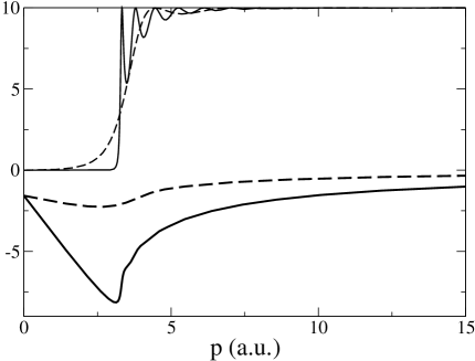
Figure 1: $\Phi_{T}$ (lower curves) and $10\times|T|^{2}$ (upper curves) versus momentum for a square barrier of “height” $V_{0}=5$ and for two different widths, $d=1$ (dashed lines), and $3$ (solid lines). $m=1$. All quantities in atomic units

As $d$ increases, the scattering resonances “above the barrier” $p>p_{0}=(2mV_{0})^{1/2}$ become more dense, and the $\pi-$jumps are better defined, because of the approach of the resonance poles in the fourth quadrant to the real axis. The corresponding increases of the phase are compensated by a more negative delay in the tunneling region.

Negative delays also arise if a pole of $T(p)$ crosses the real axis upwards, when varying the interaction strength, to become a loosely bound state in the positive imaginary axis. Levinson’s theorem de Bianchi (1994),

$$\Phi_{T}(0)=\cases{\pi(n_{b}-{1}/{2})&if $\,T(p=0)=0$\cr\pi n_{b},&if $\,\,T(p=0)\neq 0$\cr}$$ (8)

(the convention being that $\Phi_{T}(\infty)=0$, with $n_{b}$ denoting the number of bound states), imposes then a sudden jump in the phase $\Phi_{T}(0)$ that must be compensated by a strong negative slope. This effect is more important near threshold, i.e., when the pole is very close to the real axis van Dijk and Kiers (1992). Similar effects have been described for non-bound state poles in complex potential scattering Muga and Palao (1998).

Note that the effects mentioned so far (due to resonances and bound states) apply to arbitrary barriers. Universal bounds on the allowed negative delays may also be found. Whereas positive delays can be arbitrarily large, negative delays are restricted by “causality conditions” Nussenzveig (1972). Some back-of-the-envelope causality arguments may however be misleading. For example, if the total time $\tau_{T}^{Ph}(-a,a)$ is to be positive, the delay cannot be more negative than the reference free time,

$$\Delta t>-\frac{md}{p},$$ (9)

cf. Galindo and Pascual (1990,1991). In fact this bound may be violated, in particular at low energy in the proximity of a loosely bound state. This should not surprise the reader after our warning against an over-interpretation of the extrapolated time $\tau^{Ph}_{T}(-a,a)$. The flaw in the argument is the assumption of positivity of $\tau_{T}^{Ph}(-a,a)$ because of an inadequate translation from the classical trajectory case. Nevertheless, rigorous bounds have been established by Wigner himself and various authors in 3D collisions, see Martin (1981); Nussenzveig (1972) for review. In 1D collisions the following bounds hold for even potentials with finite support between $-a$ and $a$ van Dijk and Kiers (1992); de Bianchi (1994) ($k=p/\hbar$):

$$\Delta t \geq \frac{m}{\hbar k}\left\{-d-\frac{1}{2k}[\sin(2ka+2\delta_{0})-\sin(2ka+2\delta_{1})]\right\}$$ (10)

$$\geq \frac{m}{p}\left(-d-\frac{1}{k}\right).$$

which follow from the bounds for the derivatives of the phase shifts,

$${\delta_{0}}^{\prime} > -a-\frac{1}{2k}\sin[2(ka+\delta_{0})]>-a-\frac{1}{2k},$$ (11)

$${\delta_{1}}^{\prime} > -a+\frac{1}{2k}\sin[2(ka+\delta_{1})]>-a-\frac{1}{2k},$$ (12)

where the prime indicates derivative with respect to $k$. Sometimes Eqs. (10,11,12) -or their 3D analogs- are pictorially or intuitively described as the result of the classical causality condition (“the traversal time must be positive”) corrected by a term of the order of a wavelength, that takes into account the wave nature of matter, see e.g. Wigner (1955); Kriman and Ferry (1987); Nussenzveig (1972). In fact the proof, summarized in the appendix, is based on the positivity of the norm inside the barrier region, $\int_{-a}^{a}dx\,\psi_{j}(x)^{2}>0$ ($\psi_{j}(x)$ are the even and odd real -improper- eigenstates of the Hamiltonian). Alternatively, it may be obtained from the positivity of the dwell time Nussenzveig (1972); Martin (1981); de Bianchi (1994), which is in this case the true “causality principle” behind the bound. The dwell time in the case at hand is defined Büttiker (1983) as

$$\tau_{D}(-a,a)\equiv\frac{m}{\hbar k}\int_{-a}^{a}dx|\psi_{j}(x)|^{2}.$$ (13)

Note that, unlike the extrapolated phase time, this quantity does not distinguish between transmitted and reflected particles, and its positivity is directly implied by its definition.

In Eqs. (10), (11) and (12), $\delta_{j}$, $j=1,2$, are the phase shifts of the eigenvalues, $S_{j}=\exp(2i\delta_{j})$, of the $S$-matrix,

$${\bf S}(p)\equiv\left(\begin{array}[]{cc}T(p)&R(p)\\ R(p)&T(p)\end{array}\right),$$ (16)

where $R$ is the reflection amplitude. Since we are dealing with parity invariant potentials,

$$S_{0} = T+R,$$

$$S_{1} = T-R.$$ (17)

According to the bound in Eq. (10) the negative delay may be arbitrarily large for small enough momenta and may diverge at $p=0$, as it occurs when a bound state appears when making the potential more attractive van Dijk and Kiers (1992). In the absence of bound states, however, the time advancement is actually bound by Eq. (9), instead of Eq. (10). Thus, whereas the experiments looking for large traversal velocities have been frequently based on evanescent conditions in square barriers (tunneling) Ranfagni et al. (1991); Enders and Nimtz (1993b); Steinberg et al. (1993), square wells may lead to much larger advancement effects for barrier depths near the thresholds.

In the next section we will show the validity of Eq. (9) in the absence of bound states for a generic class of potentials and for all real $k$. Sassoli de Bianchi, using Levinson’s theorem, had previously pointed out the validity of Eq. (9) in the absence of bound states, but only in the limit $k\to 0$ de Bianchi (1994).

Later we will insist on the further time advancements due to bound states in the specific setting of square wells.

IV Bound without bound states

The bound for the time advancement without bound states follows from the “canonical product expansion” of the $S_{j}$. Note first that for cut-off potentials $T$ and $R$, and thus both $S_{0}$ and $S_{1}$, are meromorphic functions of $k$ in the entire complex plane Deift and Trubowitz (1979). In the absence of bound states, $S_{j}$ may only have simple poles in the lower half plane, and the corresponding zeros in the upper half plane,

$$S_{j}=\pm e^{-2ika}\prod_{n}\frac{(k-k_{j,n}^{*})(k+k_{j,n})}{(k-k_{j,n})(k+k_{j,n}^{*})}.$$ (18)

Even more, each pole $k_{j,n}$ in the fourth quadrant goes hand in hand with a twin pole at $-k_{j,n}^{*}$. This is the most general form compatible with the following properties of the $S_{j}$:

$$S_{j}(k)S_{j}^{*}(k^{*})=1,$$ (19)

$$S_{j}^{*}(k)=S_{j}(-k^{*}),$$ (20)

$$|S_{a,j}|\leq 1\;\;({\rm Im}k\geq 0),$$ (21)

where

$$S_{a,j}=e^{2ika}S_{j}.$$ (22)

The first two are the the “unitarity” and “symmetry” relations that follow from the reality of the potential, whereas the last one follows (in the absence of bound states) from van Kampen’s causality condition van Kampen (1953); Nussenzveig (1972), namely from the fact that the total probability of finding the particle outside any sphere of radius $r\geq a$ cannot be greater than one. An equivalent formulation is that the outgoing probability current, integrated from $-\infty$ to $t$, cannot exceed the integrated ingoing current by more than the absolute value of the integral of the interference (ingoing-outgoing) term. Van Kampen arrived at this causality condition noticing that the causality condition for the scattering of the Maxwell field, which implies a maximum velocity $c$, does not apply to the Schrödinger equation; moreover, no wave packets could be built which propagate with a sharp front for any finite interval of time. The mathematical arguments leading to Eq. (21) are lengthy but admit a direct translation to the two partial waves of the one dimensional case. That Eq. (21) is fulfilled may be checked in any case in the examples considered below.

Taking the logarithmic derivative on both sides of Eq. (18) one obtains,

$$d\delta_{j}/dk=-a-\sum_{n}\left(\frac{1}{|k-k_{j,n}|^{2}}+\frac{1}{|k+k_{j,n}|^{2}}\right){\rm Im}\,k_{j,n},$$ (23)

assuming that $k$ is real. Since all the poles lie in the lower half-plane the second term is positive. In the absence of bound states, $\delta_{j}^{\prime}\geq-a$ and, since $\Phi_{T}=\delta_{0}+\delta_{1}$, the transmission time delay does indeed satisfy the bound of Eq. (9).

A bound state of energy $-(\hbar K_{b})^{2}/(2m)$ for the $j$-partial wave implies for $S_{j}$ an extra factor $(k+iK_{b})/(iK_{b}-k)$, with $K_{b}>0$, which spoils the lower limit $-a$ for $\delta_{j}^{\prime}$. The contribution of these bound-state terms will however be negligible for large $k$. If there is just one bound state corresponding to a pole at $k=iK_{b}$, one obtains, similarly to the 3D case Nussenzveig (1972),

$$\Delta t\geq-\frac{m}{p}\left(d+\frac{1}{K_{b}}\right),$$ (24)

which may be interpreted in terms of an increased size of the scatterer due to the broad range of the loosely bound state.

V Examples

The above properties of the $S_{j}$ can be easily exemplified with the aid of analytically solvable models. We have in particular checked the validity of Eq. (9) for the square barrier,

$$V_{sb}(x)=V_{0}\,\chi(-a,a),$$ (25)

for $V_{0}>0$, where $\chi(-a,a)$ is the characteristic function for the barrier region.

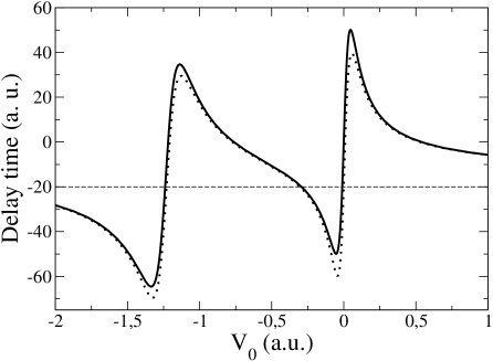
Figure 2: Time delay versus barrier height/depth for a square potential. The incident momentum is $k=0.1$, mass $m=1$, and barrier width $d=2$ (all magnitudes in atomic units). The exact expression for the time delay is depicted with a continuous line. The dotted line corresponds to the top bound of (10), whereas the dashed line is the constant quantity of the failed bound (9)

The eigenphaseshifts $\delta_{j}$ and their derivatives are easily computed as explicit functions; however, those expressions are not very enlightening for current purposes, so they are not displayed here. By making $V_{0}<0$ and allowing for the presence of bound states the bound (9) is not satisfied any more, but Eq. (10) does hold.

In order to make this explicit, we have plotted in Fig. 2 the delay time as a function of the well depth for a set value of momentum, and, so as to compare, both constant bound (9), and the more adequate Eq. (10). The line depicting the constant value $-\frac{md}{p}$ is seen to cut the computed line at points close to those that correspond to the onset of a new bound state. On the other hand, the oscillatory bound of Eq. (11) keeps track of the injection of new bound states. This effect takes place for each new bound state that comes into play; in the figure only the first two thresholds for new bound states appear, but the same structure repeats itself. Note that, as we are stressing throughout, the simple bound (9) does indeed hold for barriers ($V_{0}>0$).

The analysis of the bound has pertained to stationary waves, or, alternatively, to wavepackets highly centered in a particular momentum component. It now behooves us to check whether the enhancement of time delays can be carried over to wavefunctions more extended in momentum space (and therefore more localized in space), with some chance of being detected. For this purpose we will reexamine Eq. (6) for the case of a square well. In such a situation $|T(k)|\sim O(k)$ as $k$ tends to zero, except when the depth of the well corresponds to the threshold of a new bound state, that is to say, except when $V_{0}=-(\hbar^{2}n^{2}\pi^{2})/(8ma^{2})$. In other words, there is no stationary state with zero energy in the presence of the well, but for the exceptional threshold cases, when such a stationary state does indeed exist, as it does for the free particle case. Therefore, except for the exceptional threshold case, the integral presents no singularity. On the other hand, for those exceptional situations $|T(k)|\to 1$ as $k$ tends to zero; since the time delay does not tend to zero in that limit either, the integral will be divergent if the asymptotic initial state in momentum representation does not go zero fast enough. This should be no surprise: exactly the same divergence would take place for free motion, and for exactly the same reason, namely, the presence of $k=0$ stationary components, for which no phase time can make sense.

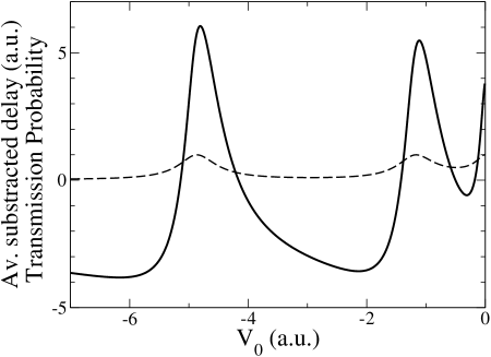
Figure 3: Transmission probability (dashed line) and averaged substracted passage time (continuous line) versus potential for a truncated gaussian wavefuncion with central momentum $k_{0}=\pi/8$ and dispersion $1.0$, whose center is located at $x_{0}=-41$ at time $t=0$. The mass of the particle is $m=1$ and the width of the square well/barrier is $d=2$. All magnitudes in atomic units.

We depict in Figure 3 the transition probability as a function of the height/depth of a square barrier/well for an asymptotic wavepacket which is gaussian in momenta, truncating out the negative momentum part, and is centered at $x_{0}=-41a$ at the instant $t=0$. For the same wavepacket we also depict the “averaged substracted passage time”, that is, the result of integral (6), minus the time that a classical particle whose momentum is the central momentum of the wavepacket would take to reach the right-hand side of the potential well, from an initial position at $x_{0}=-41a$ (the classical particle would be moving in the potential well, for adequate comparison) . The applicability of Eq. (6) is ensured by the large initial distance. Negative substracted passage times are apparent for zones of the potential strength for which a new state has just been injected into the bound sector. These negative passage times would be enhanced if the gaussian were closer to $k=0$ in momentum space, be it because the center of the wavepacket in momentum space moved towards the origin, or because the width of the packet increased. An important aspect, apparent from the figure, is that the transmission probability is big in some zones of negative average passage times. This is due to the fact that the module of the transmission amplitude, $|T(k)|$, has a maximum very close to $k=0$ if the gap from the highest lying bound state to the continuum spectrum is small. Therefore, we can have at the same time high transmission probability, and strongly enhanced negative time delays; the idea of using parameters of the potentials very close to those introducing a new bound state in order to measure negative delays immediately springs to mind.

VI Discussion

We have shown that the time advancement of the transmitted wave packet of a particle colliding with a potential barrier without bound states is bounded, due to the causality condition of van Kampen, by the simple prediction based on assuming the positivity of the extrapolated phase time. This positivity does not hold in the presence of bound states, in which case a different bound allows for large advancements al low incident energy near depth thresholds where a bound state appears (“ultra Hartman effect”). We have also argued, and provided explicit examples, that these large advancements are indeed observable, since the transmission probability is large at low energies near the thresholds.

The present approach is formally limited by the assumption of a cut-off in the potential and one may wonder about its relevance for arbitrary potentials, but it is clear that the difference between the actual (non-cut-off) potential and a potential truncated at an arbitrarily large distance from the center cannot be physically significant. Thus, even though the canonical form assumed for the $S_{j}$ in the complex plane may fail for the non-cut-off potential, all observable features associated with real and positive values of the wave number will be essentially unchanged, in particular the delay times and their bounds.

Appendix A Proof of bounds (11) and (12)

Eq. (10) may be proven by using the even and odd eigenfunctions $\psi_{j}(x)$ of the Hamiltonian, for which the boundary conditions are

$$\lim_{x\to-\infty}\psi_{0}(x) = \left(\frac{2}{h}\right)^{1/2}\cos(-px/\hbar+\delta_{0}),$$

$$\lim_{x\to\infty}\psi_{0}(x) = \left(\frac{2}{h}\right)^{1/2}\cos(px/\hbar+\delta_{0}),$$

$$\lim_{x\to-\infty}\psi_{1}(x) = \left(\frac{2}{h}\right)^{1/2}\sin(px/\hbar-\delta_{1}),$$

$$\lim_{x\to\infty}\psi_{1}(x) = \left(\frac{2}{h}\right)^{1/2}\sin(px/\hbar+\delta_{1}).$$ (26)

In particular we shall use the fact that $\int_{-a}^{a}dx\,\psi_{j}^{2}>0$. We start by calculating the logarithmic derivative of $\psi_{0}(x)$ at $x=a$ from the known expression for the outer region, see (26),

$$L_{a}\equiv\frac{\psi_{0}^{\prime}(x)}{\psi_{0}(x)}\bigg{|}_{x=a}=-\frac{p}{\hbar}\tan(pa/\hbar+\delta_{0})=-k\tan(ka+\delta_{0}),$$ (27)

where $\psi^{\prime}(x)=d\psi_{0}(x)/dx$, and henceforward the primes denote derivative wih respect to $x$. Taking the derivative of $L_{a}$ with respect to $k$,

$$\frac{d\delta_{0}}{dk}=-\frac{1}{k}\frac{dL_{a}}{dk}\cos^{2}(ka+\delta_{0})-a-\frac{1}{2k}\sin[2(ka+\delta_{0})].$$ (28)

The first term on the right hand side may also be written as

$$-\frac{\cos^{2}(ka+\delta_{0})}{k}\frac{dL_{a}}{dk} = -\frac{h}{2k}\psi_{0}^{2}(a)\left[\frac{\psi_{0}^{\prime}(x)}{\psi_{0}(x)}\right]_{k}\bigg{|}_{x=a}=$$ (29)

$$= -\frac{h}{2k}\psi_{0}(a)\tensor{\partial}_{k}\psi_{0}^{\prime}(a)=$$

$$= -\frac{h^{3}}{8\pi^{2}m}\psi_{0}(a)\tensor{\partial}_{E}\psi_{0}^{\prime}(a)\,.$$

Here and in what follows, the subscript $k$ and $E$ are shorthand notation for the derivatives with respect to $k$ and $E$, respectively, whereas the derivative with respect to $x$ is denoted by primes, and the symbol $g(x)\tensor{\partial}_{y}f(x)$ indicates $g(x)\partial_{y}f(x)-(\partial_{y}g(x))f(x)$ . Repeating the same operations for $x=-a$ one finds that

$$[\psi_{0,E}(-a)\psi_{0}^{\prime}(-a)-\psi_{0}(-a)\psi_{0,E}^{\prime}(-a)]$$ (32)

$$= -[\psi_{0,E}(a)\psi_{0}^{\prime}(a)-\psi_{0}(a)\psi_{0,E}^{\prime}(a)].$$

We shall now prove that this is a positive quantity. Taking the derivative of the stationary Schrödinger equation with respect to energy one obtains for real eigenfunctions of $H$ the identity Smith (1960)

$$\psi(x)^{2}=-\frac{\hbar^{2}}{2m}\frac{\partial}{\partial x}\left(\psi(x)\psi_{,E}^{\prime}(x)-\psi_{,E}(x)\psi^{\prime}(x)\right),$$ (33)

so that, using (32),

$$\int_{-a}^{a}dx\,\psi_{0}(x)^{2}=\frac{\hbar^{2}}{m}\left(\psi_{0,E}(a)\psi_{0}^{\prime}(a)-\psi_{0}(a)\psi_{0,E}^{\prime}(a)\right),$$ (34)

whence the positivity of $-\frac{1}{k}\frac{dL_{a}}{dk}\cos^{2}(ka+\delta_{0})$ follows, and thus bound (11) is seen to hold.

Carrying out similar manipulations for the odd wave function $\psi_{1}(x)$, and using $\Phi_{T}=\delta_{0}+\delta_{1}$, (10) is found as a consequence of the positivity of the probability to find the particle in the barrier region.