Exact isolated solutions for the two-photon Rabi Hamiltonian

Abstract

The two-photon Rabi Hamiltonian is a simple model describing the interaction of light with matter, with the interaction being mediated by the exchange of two photons. Although this model is exactly soluble in the rotating-wave approximation, we work with the full Hamiltonian, maintaining the non-integrability of the model. We demonstrate that, despite this non-integrability, there exist isolated, exact solutions for this model analogous to the so-called Juddian solutions found for the single-photon Rabi Hamiltonian. In so doing we use a Bogoliubov transformation of the field mode, as described by the present authors in an earlier publication.

PACS number(s): 03.65.-w, 42.50.-p, 32.80.-t

I Introduction

The Rabi Hamiltonian (RH), introduced by Rabi in 1937 [1], has long served as a popular and successful model of the interaction between matter and electromagnetic radiation. The Hamiltonian provides a description of an atom approximated by a two-level system interacting via a dipole interaction with a single mode of radiation [2]. Typically, this Hamiltonian is studied within the rotating-wave approximation (RWA), which results in the well-known Jaynes-Cummings model (JCM) [3]. The JCM is exactly integrable, whereas the full RH is not.

The two-photon Rabi Hamiltonian (TPRH) is an obvious extension of the original RH, where the atomic transitions are induced by the absorption and emission of two photons rather than one. Such non-linear optical processes have been of considerable interest [4], with applications including two-photon lasers and two-photon optical bistability [5]. The TPRH is not known to be integrable, whereas its RWA counterpart is, as has been demonstrated by Sukumar and Buck [6] and Compagno and Persico [7]. It should be noted from the outset that the TPRH, and its RWA variant, are phenomenological Hamiltonians, in that they neglect the effects of intensity-dependent Stark shifts of the atomic levels [8]. Nevertheless they do provide useful prototypes of two-photon interactions [9], and their similarity with the RH and its RWA variant allows fruitful comparisons to be made [10]. The TPRH has been of considerable theoretical interest due to the connection of the two-photon interaction to the group $SU(1,1)$ and to the squeezed states [11]. Experimentally, the observation of two-photon Rabi oscillations in experiments with Rydberg atoms [12, 13] has also contributed to the interest in this type of model.

Comparatively little attention has focused on the TPRH without the RWA. A notable exception to this is the work of Ng et al. [14], who have used numerical diagonalisation in a truncated basis to investigate the spectrum and simple dynamics of the system. Their analysis indicates that the spectrum of the full Hamiltonian is significantly different to the RWA spectrum, and that making the RWA also alters appreciably the dynamics. These results fit in well with other work regarding the RWA, which suggest that the consequences of making this approximation may be greater than usually thought [15, 16]. Here we shall exclusively consider the full Hamiltonian without the RWA.

In this communication we discuss a number of exact results for the TPRH without the RWA. After introducing the Hamiltonian and examining its connection to the group $SU(1,1)$, we consider the limit of the Hamiltonian in which the atomic levels become degenerate. In so doing we obtain a condition on the range of atom-field couplings for which this model remains mathematically valid. We then proceed to obtain a set of isolated, exact solutions for the Hamiltonian. Their counterparts are well known for the single-photon RH, where they are referred to as Juddian solutions [17, 18]. Such solutions tell us a great deal about the structure and symmetries of this type of non-adiabatic model. They may also serve as benchmarks for numerical techniques and as foundations for perturbative treatments. Furthermore, the existence of isolated exact solutions in non-integrable quantum models is also of interest from the perspective of studying possible quantum chaos in such systems [19, 20]. In determining these solutions for the TPRH we shall utilise an appropriate Bogoliubov transformation of the field mode, an approach outlined by the present authors in a previous publication [21], to be referred to as I hereafter.

II The Hamiltonian

The TPRH describes the interaction of a two-level atom with a single bosonic field mode via a two-photon interaction. The field is described by the annihilation and creation operators, $b$ and $b^{\dagger}$ respectively, which obey the usual commutation relation, $\left[b,b^{\dagger}\right]=1$. The two-level atom is described by the Pauli pseudo-spin operators $\left\{\sigma_{k};k=x,y,z\right\}$, which satisfy the $SU(2)$ commutation relations, $\left[\sigma_{x},\sigma_{y}\right]=2i\sigma_{z}$, plus cyclic permutations. We define the raising and lowering operators as $\sigma_{+}\equiv\sigma_{x}+i\sigma_{y}$, $\sigma_{-}\equiv\sigma_{x}-i\sigma_{y}$.

In terms of these operators, the TPRH is given by

$$H_{2\gamma}=\frac{\omega_{0}}{2}\sigma_{z}+\omega b^{\dagger}b+g\left(\left(b^{\dagger}\right)^{2}+b^{2}\right)\left(\sigma_{+}+\sigma_{-}\right),$$ (1)

where $\omega_{0}$ is the atomic level splitting, $\omega$ is the frequency of the boson mode and $g$ is the coupling strength of the atom to the field. Note that here we have the operators $\left(b^{\dagger}\right)^{2}$ and $b^{2}$ inducing atomic transitions, instead of $b^{\dagger}$ and $b$, as we would have in the single-photon RH. It is convenient to rescale the Hamiltonian as $H_{\mathrm{2\gamma}}=\omega\tilde{H}_{\mathrm{2\gamma}}$, where

$$\tilde{H}_{\mathrm{2\gamma}}=\tilde{\omega}\sigma_{z}+b^{\dagger}b+\lambda\left(\left(b^{\dagger}\right)^{2}+b^{2}\right)\sigma_{x},$$ (2)

and $\tilde{\omega}\equiv\frac{\omega_{0}}{2\omega}$ and $\lambda\equiv\frac{2g}{\omega}$. The TPRH is not known to be integrable. Like the single-photon RH, the TPRH possesses a conserved quantum number, which in the present case is $\pi_{2\gamma}$, namely an eigenvalue of the operator

$$\Pi_{2\gamma} \equiv \exp\left[\frac{i\pi}{2}\left(b^{\dagger}b+\sigma_{z}+1\right)\right]$$ (3)

$$= -\sigma_{z}\exp\left[\frac{i\pi}{2}b^{\dagger}b\right].$$ (4)

It is simple to show that $\left[H_{2\gamma},\Pi_{2\gamma}\right]=0$. The operator $\exp\left(i\frac{\pi}{2}b^{\dagger}b\right)$ is the square root of the elementary parity operator $\exp\left(i\pi b^{\dagger}b\right)=\Pi_{2\gamma}^{2}$, and has been denoted as the Fourier operator. Its role in squeezing has been described in detail elsewhere [22].

As the level-flip in the TPRH is induced by two photons, the condition for the system to be on resonance is $\omega_{0}=2\omega$, or alternatively that $\tilde{\omega}=1$.

II.1 The TPRH and the $SU(1,1)$ Group

The TPRH contains only quadratic combinations of the bosonic creation and annihilation operators. Consequently, we may write the Hamiltonian in terms of the three operators $K_{0}$, $K_{+}$ and $K_{-}$, which are defined as

$$K_{+}\equiv\frac{1}{2}\left(b^{\dagger}\right)^{2},~{}~{}~{}~{}K_{-}\equiv K_{+}^{\dagger}=\frac{1}{2}b^{2},~{}~{}~{}~{}K_{0}\equiv\frac{1}{2}b^{\dagger}b+\frac{1}{4}.$$ (5)

These operators form a closed Lie algebra $SU\left(1,1\right)$, defined by the commutator relations

$$\left[K_{0},K_{\pm}\right]=\pm K_{\pm},~{}~{}\left[K_{-},K_{+}\right]=2K_{0}.$$ (6)

The corresponding invariant Casimir operator $C$ is given by

$$C\equiv K_{0}^{2}-\frac{1}{2}\left(K_{+}K_{-}+K_{-}K_{+}\right),$$ (7)

which commutes with all three generators. For our purposes here, we shall use a unitary irreducible representation of this algebra known as the positive discrete series $\mathit{D}^{+}\left(k\right)$ [23]. In this representation the basis states $\left\{|k,m\rangle\right\}$ diagonalise the operator $K_{0}$

$$K_{0}|k,m\rangle=\left(m+k\right)|k,m\rangle,$$ (8)

for $k>0$ and $m=0,1,2,\ldots$. The action of the Casimir operator in this representation is

$$C|k,m\rangle=k\left(k-1\right)|k,m\rangle.$$ (9)

The operators $K_{+}$ and $K_{-}$ are Hermitian conjugate to each other and act as raising and lowering operators respectively within $\mathit{D}^{+}\left(k\right)$,

$$K_{+}|k,m\rangle=\sqrt{\left(m+1\right)\left(m+2k\right)}|k,m+1\rangle,$$

$$K_{-}|k,m\rangle=\sqrt{m\left(m+2k-1\right)}|k,m-1\rangle.$$ (10)

For the single-mode bosonic realisation of $SU(1,1)$ that we require here, the Bargmann index $k$ is equal to either $\frac{1}{4}$ or $\frac{3}{4}$. In terms of the original Bose operators the states $|k,m\rangle$ are given equivalently as

$$|1/4,m\rangle\equiv\frac{1}{\left(2m\right)!}\left(b^{\dagger}\right)^{2m}|0\rangle;~{}~{}~{}~{}|3/4,m\rangle\equiv\frac{1}{\left(2m+1\right)!}\left(b^{\dagger}\right)^{2m+1}|0\rangle,~{}~{}~{}m=0,1,2,\ldots.$$ (11)

So by switching to a $SU(1,1)$ representation we explicitly acknowledge that we are splitting the Hilbert space of the boson field into two independent subspaces. Each subspace is labeled by the Bargmann index $k=\frac{1}{4},\frac{3}{4}$ and only contains either all even ($k=\frac{1}{4}$) or all odd ($k=\frac{3}{4}$) number states . It is interesting to note in passing that the algebra $SU(1,1)$ may also be used to describe a system of two bosonic modes, which interact in such a way as to preserve the total particle number [25, 24]

In terms of the $SU(1,1)$ generators, the TPRH can be written

$$H_{2\gamma}=\frac{\omega_{0}}{2}\sigma_{z}+2\omega\left(K_{0}-\frac{1}{4}\right)+2g\left(K_{+}+K_{-}\right)\left(\sigma_{+}+\sigma_{-}\right),$$ (12)

with the rescaled Hamiltonian being given by

$$\tilde{H}_{\mathrm{2\gamma}}=\tilde{\omega}\sigma_{z}+2\left(K_{0}-\frac{1}{4}\right)+2\lambda\left(K_{+}+K_{-}\right)\sigma_{x}.$$ (13)

II.2 Squeezing and $SU(1,1)$

The relationship between the group $SU(1,1)$ and squeezing has been described in detail elsewhere [26] and the use of squeezed states in finding exact isolated solutions has been previously discussed in I. Here we simply note that the general squeezing operator $S$ can be written as

$$S\left(\sigma,\beta\right)=\exp\left(\sigma K_{+}\right)\left(1-|\sigma|^{2}\right)^{K_{0}}\exp\left(-\sigma^{*}K_{-}\right)\exp\left(\beta\left(K_{0}-1/2\right)\right),$$ (14)

where $\sigma$ and $\beta$ are squeezing parameters, with $\beta$ real and $\sigma$ a complex number with modulus $|\sigma|<1$. $S$ is a unitary operator, $S^{\dagger}S=1$, and provides a representation of the group $SU(1,1)$. With it we may make unitary transformations of the bosonic annihilation and creation operators, such that

$$S\left(\sigma,\beta\right)bS^{\dagger}\left(\sigma,\beta\right) = e^{-i\beta}\left(1-|\sigma|^{2}\right)^{-1/2}\left(b-\sigma b^{\dagger}\right)\equiv c,$$

$$S\left(\sigma,\beta\right)b^{\dagger}S^{\dagger}\left(\sigma,\beta\right) = e^{i\beta}\left(1-|\sigma|^{2}\right)^{-1/2}\left(b^{\dagger}-\sigma^{*}b\right)\equiv c^{\dagger}.$$ (15)

The operators $c$ and $c^{\dagger}$ satisfy the commutation relation $\left[c,c^{\dagger}\right]=1$, and are henceforth referred to as squeezed boson operators.

III Degenerate atomic levels

For degenerate atomic levels, $\omega_{0}=0=\tilde{\omega}$, the (rescaled) TPRH takes the form

$$\tilde{H}_{2\gamma}^{\left(\omega_{0}=0\right)}=b^{\dagger}b+\lambda\left(\left(b^{\dagger}\right)^{2}+b^{2}\right)\sigma_{x}.$$ (16)

Consequently eigenstates of $\tilde{H}_{2\gamma}^{\left(\omega_{0}=0\right)}$ are also eigenstates of $\sigma_{x}$, and we are led to consider the bosonic Hamiltonian,

$$\tilde{h}_{2\gamma}^{\left(\omega_{0}=0\right)}=b^{\dagger}b\pm\lambda\left(\left(b^{\dagger}\right)^{2}+b^{2}\right),$$ (17)

where the two signs correspond to the two eigenvalues of $\sigma_{x}$. The Hamiltonian of Eq. (17) has the form of a squeezed harmonic oscillator. In seeking its eigen-solutions, it is convenient to use the squeezed bosons discussed above.

Inverting the relations (15), setting $\beta$ to zero and constraining $\sigma$ to be real, we obtain the following forms for the squeezed bosonic operators

$$c^{\dagger}_{\pm}\equiv\frac{b^{\dagger}\pm\sigma b}{\sqrt{1-\sigma^{2}}},~{}~{}c_{\pm}\equiv\frac{b\pm\sigma b^{\dagger}}{\sqrt{1-\sigma^{2}}},$$ (18)

where the subscript on these operators corresponds to the sign in Eq. (17). We now choose $\sigma$ to be given by

$$\sigma=\frac{1-\Omega}{2\lambda};~{}~{}~{}~{}\Omega\equiv\sqrt{1-4\lambda^{2}}.$$ (19)

Writing the Hamiltonian in terms of these squeezed operators with this value of $\sigma$ we have

$$\tilde{h}_{2\gamma}^{\left(\omega_{0}=0\right)}=\Omega\left(c_{\pm}^{\dagger}c_{\pm}+\frac{1}{2}\right)-\frac{1}{2}.$$ (20)

The eigenstates of this Hamiltonian are clearly the number states of the $c_{\pm}$-type bosons, which we denote $|n,\mp\sigma\rangle$, such that $c_{\pm}^{\dagger}c_{\pm}|n,\mp\sigma\rangle=n|n,\mp\sigma\rangle$. In our original unsqueezed representation, these states have the form

$$|n;\mp\sigma\rangle=\frac{\left(1-\sigma^{2}\right)^{1/4}}{\sqrt{n!}}\left[\frac{b^{\dagger}\pm\sigma b}{\sqrt{1-\sigma^{2}}}\right]^{n}e^{\mp\frac{1}{2}\sigma{b^{\dagger}}^{2}}|0\rangle,$$ (21)

showing them to be the usual squeezed number states [26]. Thus we see the eigenenergies of the Hamiltonian of Eq. (20) to be

$$\tilde{E}^{(\omega_{0}=0)}_{n}=\left\{n+\frac{1}{2}\right\}\Omega-\frac{1}{2},$$ (22)

such that $\tilde{h}_{2\gamma}^{\left(\omega_{0}=0\right)}|n;\mp\sigma\rangle=\tilde{E}^{(\omega_{0}=0)}_{n}|n;\mp\sigma\rangle$.

An important feature of the TPRH is revealed by considering this $\omega_{0}=0$ case. As we saw above, the eigenfunctions of the bosonic part of the $\omega_{0}=0$ Hamiltonian are number states of the squeezed bosons. The squeezed vacuum, $|0;\mp\sigma\rangle$, is proportional to $\exp\left(\mp\frac{1}{2}\sigma{b^{\dagger}}^{2}\right)|0\rangle$ and this state is only normalisable for $|\sigma|<1$, which corresponds to the conditions

$$|\lambda|<\frac{1}{2};~{}~{}~{}~{}~{}|\frac{4g}{\omega}|<1.$$ (23)

Above this value of $g/\omega$ the $\omega_{0}=0$ Hamiltonian does not possess normalisable eigenfunctions and is thus unphysical. As has been discussed by Ng et al. [14], and as is borne out by numerical diagonalisation [27], this analysis still holds for the $\omega_{0}\neq 0$ case as the remaining operator in the Hamiltonian, $\tilde{\omega}\sigma_{z}$, is clearly a bounded operator [28], and thus presents no problems. Thus we see that the TPRH is only well defined for values of $|\lambda|<1/2$. This restriction on the coupling is not a severe restriction as, at higher couplings, effects not included in this model, such as the contributions of off-resonant, one-photon processes, will come into play, thereby compromising the physical relevance of the model.

IV Isolated exact solutions

We now demonstrate the existence of a class of isolated, exact solutions for the TPRH, similar to the Juddian solutions found for the one-photon RH. Following I we seek solutions by first performing a Bogoliubov transformation of the field mode. Bearing in mind the $\tilde{\omega}=0$ result, we shall make the transformation from the original bosons $b$ and $b^{\dagger}$ to the squeezed bosons $c$ and $c^{\dagger}$,

$$b=\left(1-\sigma^{2}\right)^{-1/2}\left(c+\sigma c^{\dagger}\right);~{}~{}b^{\dagger}=\left(1-\sigma^{2}\right)^{-1/2}\left(\sigma c+c^{\dagger}\right),$$ (24)

where we have assumed that $\beta=0$ and that $\sigma$ is real and to be determined. The justification of this is provided by subsequent results.

With this change in bosonic representation, the rescaled TPRH becomes

$$\tilde{H}_{2\gamma}=\tilde{\omega}\sigma_{z} + \frac{1}{\kappa}\left(\sigma c^{2}+\sigma{c^{\dagger}}^{2}+\left(1+\sigma^{2}\right)c^{\dagger}c+\sigma^{2}\right)$$ (25)

$$+ \frac{\lambda}{\kappa}\left(\left(1+\sigma^{2}\right)\left({c^{\dagger}}^{2}+c^{2}\right)+4\sigma c^{\dagger}c+2\sigma\right)\sigma_{x},$$

where $\kappa\equiv\left(1-\sigma^{2}\right)$. We now use an appropriate matrix representation for the Pauli matrices, which for this model is one in which $\sigma_{x}$ is diagonal. We use

$$\sigma_{x}=\left[\begin{array}[]{lr}1&0\\ 0&-1\end{array}\right],~{}~{}\sigma_{y}=\left[\begin{array}[]{lr}0&i\\ -i&0\end{array}\right],~{}~{}\sigma_{z}=\left[\begin{array}[]{lr}0&1\\ 1&0\end{array}\right].$$ (26)

In terms of the two-component wavefunction, $|\Psi\rangle={|\Psi_{1}\rangle\choose|\Psi_{2}\rangle}$, the time-independent Schrödinger equation for the system, $\tilde{H}_{\mathrm{2\gamma}}|\Psi\rangle=\tilde{E}|\Psi\rangle$, where $\tilde{E}\equiv E/\omega$ is the rescaled energy, then reads

$$\tilde{\omega}|\Psi_{2}\rangle + \frac{1}{\kappa}\left\{\left[\sigma+\lambda\left(1+\sigma^{2}\right)\right]\left({c^{\dagger}}^{2}+c^{2}\right)\right.$$ (27)

$$\left.+\left[1+\sigma^{2}+4\lambda\sigma\right]c^{\dagger}c+\sigma^{2}+2\lambda\sigma-\kappa\tilde{E}\right\}|\Psi_{1}\rangle=0,$$

$$\tilde{\omega}|\Psi_{1}\rangle + \frac{1}{\kappa}\left\{\left[\sigma-\lambda\left(1+\sigma^{2}\right)\right]\left({c^{\dagger}}^{2}+c^{2}\right)\right.$$ (28)

$$\left.+\left[1+\sigma^{2}-4\lambda\sigma\right]c^{\dagger}c+\sigma^{2}-2\lambda\sigma-\kappa\tilde{E}\right\}|\Psi_{2}\rangle=0$$

It is immediately clear that if we set either $\left[\sigma+\lambda\left(1+\sigma^{2}\right)\right]$ or $\left[\sigma-\lambda\left(1+\sigma^{2}\right)\right]$ equal to zero, we make a determination of $\sigma$ and reduce either Eq. (27) or Eq. (28) considerably. Choosing the first of these options, we have

$$\sigma+\lambda\left(1+\sigma^{2}\right)=0$$ (29)

which gives

$$\sigma=\frac{-1\pm\Omega}{2\lambda},$$ (30)

where $\Omega$ is as defined previously in Eq. (19). In order that $|\sigma|<1$, we must henceforth choose the positive sign in Eq. (30), so that $\sigma\rightarrow 0$ as $\lambda\rightarrow 0$. Thus our squeezing parameter is

$$\sigma=\frac{\Omega-1}{2\lambda}.$$ (31)

Note that had we pursued the other option and set $\left[\sigma-\lambda\left(1+\sigma^{2}\right)\right]=0$, we would have obtained the same determination of the squeezing parameter as for the $\omega_{0}=0$ case given by Eq. (19). This second solution will be discussed later. Proceeding with this choice of squeezing given by Eq. (31), Eqs. (27) and (28) become

$$\tilde{\omega}|\Psi_{2}\rangle + \left\{\Omega c^{\dagger}c-\left[\tilde{E}+\frac{1}{2}-\frac{\Omega}{2}\right]\right\}|\Psi_{1}\rangle=0,$$ (32)

$$\tilde{\omega}|\Psi_{1}\rangle + \frac{1}{\Omega}\left\{-\sqrt{1-\Omega^{2}}\left({c^{\dagger}}^{2}+c^{2}\right)+\left(2-\Omega^{2}\right)c^{\dagger}c\right.$$ (33)

$$\left.+\frac{1}{2}\left(1-\Omega\right)\left(2+\Omega\right)-\Omega\tilde{E}\right\}|\Psi_{2}\rangle=0.$$

For $|\Psi_{1}\rangle$ and $|\Psi_{2}\rangle$ we now choose simple Ansätze in terms of the squeezed number states;

$$|\Psi_{1}\rangle=\sum_{n=0}^{N}p_{n}|n;\sigma\rangle,$$ (34)

$$|\Psi_{2}\rangle=\sum_{m=0}^{N-2}q_{m}|m;\sigma\rangle,$$ (35)

which gives us the equations

$$\sum_{m=0}^{N-2}\tilde{\omega}q_{m}|m;\sigma\rangle + \sum_{n=0}^{N}p_{n}\left\{n\Omega-\left[\tilde{E}+\frac{1}{2}-\frac{\Omega}{2}\right]\right\}|n;\sigma\rangle=0,$$ (36)

$$\sum_{n=0}^{N}\tilde{\omega}p_{n}|n;\sigma\rangle + \sum_{m=0}^{N-2}q_{m}\frac{1}{\Omega}\left\{-\sqrt{1-\Omega^{2}}\left[\sqrt{\left(m+1\right)\left(m+2\right)}|m+2;\sigma\rangle\right.\right.$$ (37)

$$\left.\left.+\sqrt{m\left(m-1\right)}|m-2;\sigma\rangle\right]+\left(2-\Omega^{2}\right)m|m;\sigma\rangle\right.$$

$$\left.+\frac{1}{2}\left[\left(1-\Omega\right)\left(2+\Omega\right)-2\Omega\tilde{E}\right]|m;\sigma\rangle\right\}=0$$

For the first equation to hold, we must have

$$p_{N}\left\{N\Omega-\left[\tilde{E}+\frac{1}{2}-\frac{\Omega}{2}\right]\right\}=0.$$ (38)

As $p_{N}\neq 0$ by Ansatz, we must have $\Omega N-\left(\tilde{E}+\frac{1}{2}-\frac{\Omega}{2}\right)=0$. This establishes the so–called energy baselines as

$$\tilde{E}=-\frac{1}{2}+\left(N+\frac{1}{2}\right)\Omega.$$ (39)

Equating the remaining coefficients of the number states in Eqs. (36) and (37) gives us the following set of equations

$$\tilde{\omega}q_{m} + \left(m-N\right)\Omega p_{m}=0;~{}~{}~{}~{}~{}~{}~{}~{}~{}~{}~{}~{}~{}~{}~{}~{}~{}~{}~{}~{}~{}~{}~{}~{}~{}~{}~{}~{}~{}~{}~{}~{}~{}~{}~{}~{}~{}~{}0\leq m\leq N-2,$$ (40)

$$\tilde{\omega}p_{n} - \frac{\sqrt{1-\Omega^{2}}}{\Omega}\sqrt{n\left(n-1\right)}q_{n-2}-\frac{\sqrt{1-\Omega^{2}}}{\Omega}\sqrt{\left(n+1\right)\left(n+2\right)}q_{n+2}$$ (41)

$$+ \frac{1}{\Omega}\left[n+1-\left(2n+N+1\right)\Omega^{2}\right]q_{n}=0;~{}~{}~{}~{}~{}~{}~{}~{}~{}~{}~{}~{}~{}~{}~{}~{}~{}~{}~{}~{}0\leq n\leq N.$$

where $q_{n}=0$ for $n<0$ and $n>N-2$. From the second of these equations we see that the Hamiltonian in this squeezed representation only couples number states that are different by multiples of two (for example it couples $|n;\sigma\rangle$ to $|n+2;\sigma\rangle$ and $|n+4;\sigma\rangle$ but not to $|n+3;\sigma\rangle$). Therefore our Ansätze need only include either all even number states or all odd number states. This is equivalent to restricting the solutions to a sector of the Hilbert space with a given Bargmann index, $k$. We also see that the minimum value of $N$ is 2. When $N$ is even, we obtain $N+1$ equations for the $N+1$ coefficients $p_{n};~{}n=0,2,\ldots,N,~{}~{}~{}q_{m};~{}m=0,2,\ldots N-2$. When $N$ is odd, we obtain $N$ equations for the $N$ coefficients $p_{n};n=1,3,\ldots,N,~{}~{}q_{m};m=1,3,\ldots N-2$. Requiring that the determinants of these equation sets are equal to zero gives us the compatibility conditions which establish the location of the Juddian points on the energy baselines. These conditions for the first three values of $N$ are:

$$2-6\Omega^{2}+\tilde{\omega}^{2} = 0;~{}~{}~{}~{}N=2,$$

$$6-10\Omega^{2}+\tilde{\omega}^{2} = 0;~{}~{}~{}~{}N=3,$$

$$8\left(3-30\Omega^{2}+35\Omega^{4}\right)+2\left(7-17\Omega^{2}\right)\tilde{\omega}^{2}+\tilde{\omega}^{4} = 0;~{}~{}~{}~{}N=4.$$ (42)

For $N$ even we have a polynomial of the order $\frac{N}{2}$ in $\tilde{\omega}^{2}$ and $\Omega^{2}$, and hence $\lambda^{2}$. For $N$ odd, the corresponding polynomial is of order ($\frac{N-1}{2}$). The equations are symmetric under $\tilde{\omega}\rightarrow-\tilde{\omega}$ or $\lambda\rightarrow-\lambda$, as expected. The solutions of these polynomials locate the exact solution in $\tilde{\omega}$–$\lambda$ space.

As in the one-photon case, there exists another degenerate solution at every Juddian point. This solution can be found by placing $\left[\sigma-\lambda\left(1+\sigma^{2}\right)\right]=0$ rather than $\left[\sigma+\lambda\left(1+\sigma^{2}\right)\right]=0$ into Eqs. (27) and (28). This simply interchanges the equations and hence the roles of $\Psi_{1}$ and $\Psi_{2}$.

V Results and Discussion

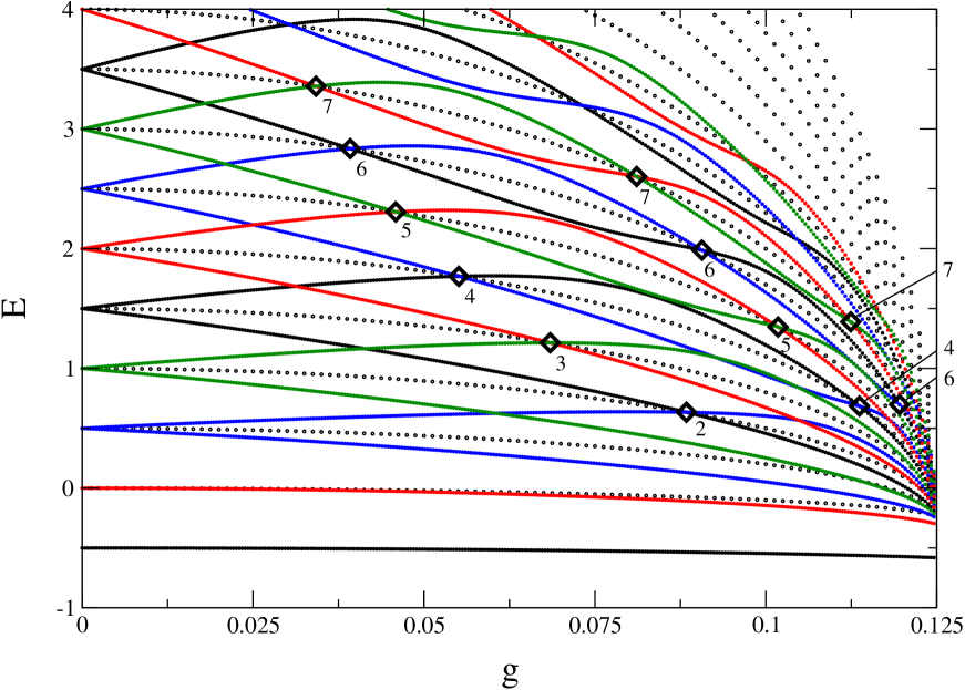
Figure 1: The first twelve Juddian points (diamonds) of the two-photon Rabi Hamiltonian determined by the method outlined in the text, plotted against the energy spectrum determined numerically (solid lines). Also plotted are the energy baselines (dotted lines). Each point is labeled with its order $N$. The Hamiltonian is resonant; $2\omega=\omega_{0}=1$.

Solving the above complementary conditions we have calculated twelve Juddian points for the resonant TPRH with $2\omega=\omega_{0}=1$, corresponding to values of of $2\leq N\leq 7$. These are displayed in Table 1, listed to the first 10 significant figures, and we have used the original units of Eq. (1). The $N=2$ and $N=3$ cases have such simple complementary conditions that closed analytic expressions may be found. On resonance these are given by $g=\frac{1}{8\sqrt{2}}$ and $E=\frac{1}{4}\left(\frac{5}{\sqrt{2}}-1\right)$ for $N=2$, and $g=\frac{1}{8}\sqrt{\frac{3}{10}}$ and $E=\frac{1}{4}\left(7\sqrt{\frac{7}{10}}-1\right)$ for $N=3$. This set of twelve Juddian points is indicated on the energy schema of the Hamiltonian in Fig. 1, where the schema was obtained by approximate numerical diagonalisation via a standard configuration-interaction method, using a basis size of the lowest 501 harmonic oscillator states [27]. The energy baselines, $E=\frac{1}{2}\left(-\frac{1}{2}+\left(N+\frac{1}{2}\right)\Omega\right)$, are also plotted.

As is clearly seen from Fig. 1, the Juddian solutions found by this method occur at level-crossings in the energy schema, but that they do not cover every crossing, as is the case with the one-photon Hamiltonian. Considering the quantum numbers $\pi_{2\gamma}$ of the two intersecting lines at each crossing, we see that the above type of solution can only describe the crossings of states having $\pi_{2\gamma}=+1$ with ones having $\pi_{2\gamma}=-1$, and of crossings of states having $\pi_{2\gamma}=+i$ with ones having $\pi_{2\gamma}=-i$. The remaining four types of possible crossings are not described. This situation is summarised in Table 2.

This series of crossings can be understood by considering the parity operator $\Pi_{2\gamma}^{2}$

$$\Pi_{2\gamma}^{2}=\exp\left(i\pi b^{\dagger}b\right),$$ (43)

which obviously commutes with the Hamiltonian. From considering the eigenvalues of this operator we see that the Juddian solutions we have described occur between levels which have the same value of $\Pi_{2\gamma}^{2}$. Thus although the Ansätze of the Juddian solutions above are not eigenstates of the Fourier-like operator $\Pi_{2\gamma}$, they are eigenstates of parity.

These crossings can be viewed in another way. Ng et al. have introduced a unitary transformation which decouples the spin and bosonic degrees of freedom [14]. After the application of this transformation, the bosonic part of the Hamiltonian is given by

$$h^{(M)}=\frac{1}{2}M\omega_{0}\left(-1\right)^{K_{0}-k}+2\omega\left(K_{0}-\frac{1}{4}\right)+4g\left(K_{+}+K_{-}\right),$$ (44)

where the numbers $M=\pm 1$, corresponding to the spin degree of freedom, and $k=\frac{1}{4},\frac{3}{4}$, corresponding to the Bargmann index, serve to characterize the four independent sub-spaces into which the full Hilbert space of the Hamiltonian decomposes under this transformation. We thus see that the crossings detailed above occur between states with the same Bargmann $k$ index, but with different $M$ indices. By contrast the missing crossings occur between states with different values of $k$.

The reason why the above Ansätze can describe these solutions and not the others is as follows. The solutions that we have been able to find occur at crossings between energy eigenfunctions that both have the same Bargmann index $k$, which means that both states are composed of either all even or all odd number states. At the Juddian points these two eigenstates become degenerate in energy and thus, to find the energy at the level-crossing we may form a linear superposition of the two eigenstates, which will, in general, not be an eigen-state of $\Pi_{2\gamma}^{2}$. Because the degenerate energy eigenstates belong to the same $k$-sector, the formation of the superposition allows the individual terms in one wavefunction to add to the terms in the other. If we form the superposition correctly, the resultant wavefunction may have a form much simpler than the constituent wavefunctions. This is exactly the case when we choose the Ansatz (35).

The solutions that we have been unable to find with the above method occur at the level-crossings between energy eigenstates that have different Bargmann indices. This means that one eigenstate is composed of odd number states, whilst the other is composed only of even number states. Consequently, no superposition of these states will lead to a reduction in the complexity of either wavefunction and we have been unable to find simple Ansätze at these level-crossings.

Although the above method is not directly extensible to the remaining crossings, it may still be the case that exact solutions can be found. Although there is no a priori reason to expect that these exact solutions exist, by looking at the energy schema generated numerically, we observe that the remaining level-crossings appear to lie along base-lines described by

$$\tilde{E}=-\frac{1}{2}+n\Omega,~{}~{}~{}~{}~{}~{}~{}n=2,3,\ldots,$$ (45)

where, as previously, $\Omega=\sqrt{1-4\lambda^{2}}$. These baselines are so similar to the baselines for the Juddian solutions found above that it would seem likely that Juddian solutions could also be found at these remaining crossings.

VI Conclusions

We have shown that a set of isolated, exact solutions exists for the two-photon Rabi Hamiltonian. These are seen to occur at a sub–set of the level-crossings in the energy schema and although we have not described every level crossing, we have been able to explain this in terms of the symmetry properties of the crossing states.

This type of isolated solution also occurs in the single-photon Rabi Hamiltonian, where they are referred to as Juddian solutions. Several methods have been proposed for finding these solutions [18, 29]. In I we have given a method for finding these solutions that is directly analogous to the one used here, except that for the one-photon case we have used displaced, rather than squeezed, bosons. In this case, the Ansatz does provide solutions at every level-crossing in the spectrum. It should be noted that the single-photon Hamiltonian is a simpler model than the TPRH, as the conserved quantum number analogous to $\pi_{2\gamma}$ only has two eigenvalues, and thus there is only one type of level crossing, whereas in the current model $\Pi_{2\gamma}$ has four eigenvalues and there are six different types of crossing.

It is hoped that the results presented here, in conjunction with those in I, will be of use in the analysis of this kind of non-adiabatic model. These isolated solutions seem an ideal starting point for the analysis of this kind of situation, since they provide exact results which may be used as bench-marks for further methods. They also provide crucial insight into the symmetries of the model.

VII Acknowledgments

One of us (C. E.) acknowledges the financial support of a research studentship from the Engineering and Physical Sciences Research Council (EPSRC) of Great Britain.

$N$	$g$	$E$
2	0.08838834765	0.6338834765
3	0.06846531969	1.214155046
4	0.1136829135	0.6855144259
4	0.05510006004	1.769611501
5	0.1017761788	1.346571001
5	0.04587381623	2.308117863
6	0.1195668196	0.6977617553
6	0.09065527261	1.987605007
6	0.03920841953	2.835982030
7	0.1124265002	1.389132039
7	0.03419600455	3.356947455
7	0.08111783821	2.603139795

Table 1: The couplings ($g$), energies ($E$), as well as order ($N$)of the first twelve Juddian points of the resonant two-photon Rabi Hamiltonian ($2\omega=\omega_{0}=1$).

	$+1$	$+i$	$-1$	$-i$
$+1$	-	n	y	n
$+i$	n	-	n	y
$-1$	y	n	-	n
$-i$	n	y	n	-

Table 2: Description of the parities of the level-crossings described by the TPRH Juddian solutions presented here. “y” denotes that the crossing is described, “n” that it is not, whereas “-” indicates that no such crossing occurs.

References

- [1] I. I. Rabi, Phys. Rev. 51, 652 (1937).
- [2] L. Allen and J. H. Eberly, Optical Resonance and Two-Level Atoms, (Wiley, New York, 1975).
- [3] E. T. Jaynes and F. W. Cummings, Proc. IEEE 51, 89 (1963).
- [4] Y. R. Shen, Phys. Rev. 155, 921 (1967); D. F. Walls, J. Phys. A 4, 813 (1971).
- [5] M. Reid, K. J. McNeil, and D. F. Walls, Phys. Rev. A 24, 2029 (1981).
- [6] C. V. Sukumar and B. Buck, Phys. Lett. A 83, 211 (1981); J. Phys. A 17, 885 (1984).
- [7] G. Compagno and F. Persico in “Coherence and Quantum optics V”, edited by L. Mandel and E. Wolf (p.1117, Plenum 1984).
- [8] R. R. Puri and R. K. Bullough, J. Opt. Soc. Am. B 5, 2021 (1988).
- [9] A. H. Toor and M. S. Zubairy, Phys. Rev. A 45, 4951 (1992)
- [10] M. Fang and P. Zhou, J. Mod. Opt. 42, 1199 (1995).
- [11] C. C. Gerry, Phys. Rev. A 37, 2683 (1988); C. C. Gerry and P. J. Moyer, ibid 38, 5665 (1988).
- [12] T. R. Gentile, B. J. Hughey, D. Kleppner, and T. W. Ducas, Phys. Rev. A 40, 5103 (1989).
- [13] M. Gatze, M. C. Baruch, R. B. Watkins, and T. F. Gallagher, Phys. Rev. A 48, 4742 (1993).
- [14] K. M. Ng, C. F. Lo, and K. L. Liu, Eur. Phys. J. D 6, 119 (1999); C. F. Lo, K. L. Liu, and K. M. Ng, Europhys. Lett. 42, 1 (1998).
- [15] I. D. Feranchuk, L. I. Komarov, and A. P. Ulyanenkov, J. Phys. A: Math. Gen. 29, 4035, (1996).
- [16] G. W. Ford and R. F. O’Connell, Physica A 243, 377 (1997).
- [17] B. R. Judd, J. Chem. Phys. 67, 1174 (1977); J. Phys. C: Solid State Phys. 12, 1685 (1979).
- [18] H. G. Reik, H. Nusser, and L. A. Amarante Ribeiro, J. Phys. A: Math. Gen. 15, 3491 (1982); M. Kuś, J. Math. Phys. 26, 2792 (1985); H. G. Reik and M. Doucha, Phys. Rev. Lett 57, 787 (1986); H. G. Reik, P. Lais, M. E. Stützle, and M. Doucha, J. Phys. A: Math. Gen 20, 6327 (1987).
- [19] R. Graham and M. Höhnerbach, Phys. Lett. A 101, 61 (1984).
- [20] G. Hose and H. S. Taylor, Phys. Rev. Lett. 51, 947 (1983).
- [21] C. Emary and R. F. Bishop, J. Math. Phys. 43, 3916 (2002).
- [22] R. F. Bishop and A. Vourdas, Phys. Rev. A 50, 4488 (1994)
- [23] A. Perelomov, Generalised Coherent States and Their Applications, (Springer, Berlin, 1986).
- [24] C. C. Gerry and R. Grobe, Phys. Rev. A 51, 4123 (1995).
- [25] R. F. Bishop and A. Vourdas, Z. Phys. B 17, 527 (1988).
- [26] R. F. Bishop and A. Vourdas, J. Phys. A: Math. Gen. 19, 2525 (1986).
- [27] C. Emary, PhD Thesis, UMIST, Manchester, 2001 (unpublished).
- [28] M. Reed and B. Simon, Methods of Modern Mathematical Physics Vol. 1: Functional Analysis (Academic, New York 1972).
- [29] M. Kuś, J. Math. Phys. 26, 2792 (1985); M. Kuś and M. Lewenstein, J. Phys. A: Math. Gen. 19, 305 (1986).