Relativistic coherent states and charge structure of the coordinate and momentum operators

Abstract

We consider relativistic coherent states for a spin-$0$ charged particle that satisfy the next additional requirements: (i) the expected values of the standard coordinate and momentum operators are uniquely related to the real and imaginary parts of the coherent state parameter $\alpha$; (ii) these states contain only one charge component. Three cases are considered: free particle, relativistic rotator, and particle in a constant homogeneous magnetic field. For the rotational motion of the two latter cases, such a description leads to the appearance of the so-called nonlinear coherent states.

I Introduction

Coherent states are currently very interesting in modern quantum physics and in quantum technologies. They have a long history and a very wide field of application. It was Schrödinger who first considered these states for the harmonic oscillator in the early years of quantum mechanics b1 . These states minimize the uncertainty relations and one of their important properties is temporal stability. It means that time evolution can be described, in this case, by changing the parameter of the coherent states

$$\alpha\longmapsto\alpha\exp\left(-i\omega t\right).$$ (1)

These states are eigenstates of the annihilation operator

$$\hat{a}=\frac{1}{\sqrt{2}}\left(\frac{\hat{q}}{\sigma}+i\frac{\sigma}{\hbar}\hat{p}\right),$$ (2)

where $\sigma=\sqrt{\hbar/m\omega}$ is a characteristic oscillator length, with eigenvalues $\alpha$,

$$\hat{a}\left|\alpha\right\rangle=\alpha\left|\alpha\right\rangle.$$ (3)

Another significant property of the coherent states is the resolution of unity b2 ; b3 . It means the existence of an integral measure $d\mu(\alpha)$ such that the following condition is satisfied:

$$\int\left|\alpha\right\rangle d\mu(\alpha)\left\langle\alpha\right|=1.$$ (4)

For the standard coherent states determined by Eq. (3) this measure has a simple form:

$$d\mu(\alpha)=\frac{d\alpha^{\prime}d\alpha^{\prime\prime}}{\pi},$$ (5)

where $\alpha^{\prime}$ and $\alpha^{\prime\prime}$ are the real and imaginary parts of the parameter $\alpha$.

These coherent states (we denote them as the standard coherent states here) can be used not only for a harmonic oscillator but for a wide enough class of the quantum systems. However, the property of the temporal stability is intrinsic to the systems which are unitarily equivalent to the harmonic oscillator. This property can be conserved by a redefinition of the coherent states b4 ; b5 .

A lot of different generalizations of the coherent states are well known today. We note only one of them that will appear in our consideration from an unexpected side. In b6 the authors have shown that trapped electron can be described by means of coherent states which are eigenstates of the deformed annihilation operator $\hat{a}_{f}$ expressed in terms of the usual annihilation and creation operators in the following way:

$$\hat{a}_{f}=\hat{a}f\left(\hat{a}^{{\dagger}}\hat{a}\right),$$ (6)

where $f$ is a certain function. Mathematical properties and a physical sense of these states have been considered in detail in b7 . The authors call these states nonlinear (or $f$) coherent states. Analogous states that satisfy the condition of temporal stability have been presented in b4 ; b5 .

The description of a relativistic quantum system by means of the coherent states meets certain difficulties. First of all, it should be noticed that relativistic quantum theory can be developed in a consistent way with the second quantization method only. It is possible to consider the one-particle sector of the theory under conditions when particle pair creation is impossible (free particle and particle in a constant magnetic field). However, even in this case the coordinate (and, generally speaking, the momentum) operator is not well defined b8 ; b9 ; b10 . This reveals itself in the fact that eigenstates of this operator contain states with different signs of charge. Therefore, the coherent states defined by Eq. (3) contain eigenstates of the Hamiltonian with different signs of charge as well. The existence of such kind of states is prohibited by the charge superselection rule b11 .

Coherent states for relativistic spin-$0$ and spin-$1/2$ particles in a constant homogeneous magnetic field have been introduced in b12 . These states are expanded in eigenstates of the Hamiltonian with one sign of charge only. However, these states are not eigenstates of the annihilation operator, and furthermore, expected values of coordinate and momentum for these states are not $\alpha^{\prime}\sqrt{2}\sigma$ and $\alpha^{\prime\prime}\sqrt{2}\hbar/\sigma$, respectively.

The coherent states for charged spin-$0$ particles which we consider in this work in detail, have been presented in b13 . These states satisfy two additional conditions:

1. The coherent state parameter $\alpha$ is expressed in terms of the mean value of the standard (not Newton – Wigner) coordinate and momentum in the usual way,

   $$\alpha=\frac{1}{\sqrt{2}}\left(\frac{\bar{q}}{\sigma}+i\frac{\sigma}{\hbar}\bar{p}\right).$$ (7)

2. These states are expanded in eigenstates of the Hamiltonian with one sign of charge only.

The coherent states, which can be constructed by using Eq. (3), satisfy condition (1) but do not satisfy condition (2); the coherent states presented in b12 , in contrast, satisfy condition (2) but do not satisfy condition (1).

In this work we consider a spin-$0$ charged particle in a constant homogeneous magnetic field and two more simple examples: free particle and relativistic rotator. These systems can be described in the one-particle sector of the theory because particle pair creation is absent there. However, the nontrivial charge structure of the coordinate and momentum operators leads to the appearance of some peculiarities in the evident form of the relativistic coherent states and in the expected values of some observables.

II Statement of the problem and charge structure of operators

Consider a scalar charged particle in a constant homogeneous magnetic field. Such a particle is described by the Klein–Gordon equation:

$$-\hbar^{2}\partial_{t}^{2}\psi=\left[c^{2}\left(\mathbf{\hat{p}}-e\mathbf{A}\left(\mathbf{\hat{r}}\right)\right)^{2}+m^{2}c^{4}\right]\psi.$$ (8)

This is a second-order equation in time. Hence, in the present form, one cannot interpret it as a Schrödinger equation. This problem can be resolved, if by means of changing

$$\psi=\frac{1}{\sqrt{2}}\left(\varphi+\chi\right),$$ (9)

$$i\hbar\partial_{t}\psi=\frac{mc^{2}}{\sqrt{2}}\left(\varphi-\chi\right)$$ (10)

one comes to the two-component wave function

$$\Psi=\left(\begin{array}[]{c}\varphi\\ \chi\end{array}\right).$$ (11)

Now, Eq. (8) can be written as the Schrödinger equation

$$i\hbar\partial_{t}\Psi=\hat{H}^{mf}\Psi,$$ (12)

where the Hamiltonian $\hat{H}^{mf}$ has the following form:

$$\hat{H}^{mf}=\left(\tau_{3}+i\tau_{2}\right)\frac{\left(\mathbf{\hat{p}}-e\mathbf{A}\left(\mathbf{\hat{r}}\right)\right)^{2}}{2m}+\tau_{3}mc^{2}.$$ (13)

In this expression $\tau_{i}$ are the $2\times 2$ matrices

$$\tau_{1}=\left(\begin{array}[]{cc}0&1\\ 1&0\end{array}\right),i\tau_{2}=\left(\begin{array}[]{cc}0&1\\ -1&0\end{array}\right),\tau_{3}=\left(\begin{array}[]{cc}1&0\\ 0&-1\end{array}\right).$$ (14)

Corresponding formalism has been presented by Feshbach and Villars in Ref. b10 .

Choose the vector potential in the form:

$$\mathbf{A}\left(\mathbf{r}\right)=\frac{1}{2}\left[\mathbf{B}\times\mathbf{r}\right],$$ (15)

where $\mathbf{B}$ has only a $z$ component

$$\mathbf{B}=\left(\begin{array}[]{c}0\\ 0\\ B\end{array}\right).$$ (16)

In this case the Hamiltonian (13) can be written as follows:

$$\hat{H}^{mf}=\left(\tau_{3}+i\tau_{2}\right)\left(\frac{\hat{p}_{z}^{2}}{2m}+\hbar\omega\left(\hat{n}+\frac{1}{2}\right)\right)+\tau_{3}mc^{2},$$ (17)

where

$$\hat{n}=\frac{1}{\hbar\omega}\left(\frac{\hat{p}^{2}}{2m}+\frac{m\omega^{2}}{2}\hat{q}^{2}\right)-\frac{1}{2}.$$ (18)

Here $\omega=eB/m$ is the cyclotron frequency. $\hat{p}$ and $\hat{q}$ are momentum and coordinate after a standard linear transformation b14 ,

$$\hat{q}=\frac{1}{\sqrt{2}}\left(\hat{y}+\frac{\hat{p}_{x}}{m\omega}\right),$$

$$\hat{p}=\frac{1}{\sqrt{2}}\left(\hat{p}_{y}-m\omega\hat{x}\right).$$ (19)

Their physical sense is coordinates of a particle in a frame connected with the center of the rotational motion (it is clear that momentum should be redefined in the corresponding units for such interpretation). One more degree of freedom vanishes in the Hamiltonian after linear transformation. The physical sense of the corresponding momentum and coordinate

$$\hat{Q}=\frac{1}{\sqrt{2}}\left(\hat{y}-\frac{\hat{p}_{x}}{m\omega}\right),$$

$$\hat{P}=\frac{1}{\sqrt{2}}\left(\hat{p}_{y}+m\omega\hat{x}\right)$$ (20)

is of coordinates of the gyration center.

First of all, consider briefly the well-known example of a one-dimensional free particle. The Hamiltonian of this system has the following form:

$$\hat{H}^{fp}=\left(\tau_{3}+i\tau_{2}\right)\frac{\hat{p}^{2}}{2m}+\tau_{3}mc^{2}.$$ (21)

It is difficult to outline an evident physical meaning for each of the components of the wave function in this representation (we denote it as the standard representation). However, the matrix of the Hamiltonian (21) can be diagonalized to the form:

$$\hat{H}^{fp}=\tau_{3}E(\hat{p}),$$ (22)

where

$$E(p)=\sqrt{m^{2}c^{4}+c^{2}p^{2}}.$$ (23)

One can provide the transformation in this representation (the Feshbach–Villars representation) using the following transform matrix:

$$\hat{U}(\hat{p})\!=\!\frac{1}{2\sqrt{mc^{2}E(\hat{p})}}\left[\left(E(\hat{p})+mc^{2}\right)+\left(E(\hat{p})-mc^{2}\right)\tau_{1}\right].$$ (24)

The components of the wave function have a sense of the solutions with positive and negative energies in the Feshbach–Villars representation.

The coordinate operator in the Feshbach–Villars representation has the even and odd (diagonal and nondiagonal) parts b8 ; b9 ; b10 , and can be written in the following form:

$$\hat{q}=i\hbar\partial_{p}-i\frac{\hbar c^{2}p}{2E^{2}(p)}\tau_{1}.$$ (25)

Such a complicated form of the operator we refer to here as the nontrivial charge structure of the coordinate operator.

Consider this question closely. It is clear that in our case all operators are $2\times 2$ operator-valued matrices. In the Feshbach–Villars representation relevant indices correspond to different signs of charge (particle or anti-particle). Operators with a nontrivial charge structure (including operator of coordinate) are not observables from the point of the charge superselection rule. Indeed, the measurement of such an operator shall result in a charge-violating state. However, it is impossible to build the modern physical theory without such operators. Most probably the measurement procedure for these provides a system from a single-particle state to a many-particle one (i.e., it results in the creation of particle pairs).

On the other hand, the state before measurement is a single-particle one and is not a superposition of states with different signs of charge. Hence, the mean of any operator depends on its even part only (diagonal matrix elements in the charge space). Therefore, only the even part of the operator is observable. Detailed consideration of this question has been presented in the work b14a .

One can write the even part of the coordinate operator as follows:

$$\left[\hat{q}\right]=i\hbar\partial_{p}.$$ (26)

It is very important that in this case the even part of the coordinate operator coincides with the Newton–Wigner position operator $\hat{\xi}$, i.e.,

$$\left[\hat{q}\right]=\hat{\xi}.$$ (27)

The momentum operator in the Feshbach–Villars representation can be written in the very simple form

$$\hat{p}=-i\hbar\partial_{\xi}.$$ (28)

Now, consider another, more complicated, example – a relativistic rotator, i.e, a particle in a constant homogeneous magnetic field without translational motion along the $z$ axis. In this case, one can write the Hamiltonian as follows:

$$\hat{H}^{r}=\hbar\omega\left(\tau_{3}+i\tau_{2}\right)\left(\hat{n}+\frac{1}{2}\right)+\tau_{3}mc^{2}.$$ (29)

This Hamiltonian can be written in the Feshbach–Villars representation (see b10 and Table 1), where it has a nontrivial charge structure. We use here another representation b15 , where the Hamiltonian (29) has a diagonal form. One can write the transform matrix in this representation as follows:

$$\hat{U}(\hat{n})\!=\!\frac{1}{2\sqrt{mc^{2}E(\hat{n})}}\!\left[\left(E(\hat{n})+mc^{2}\right)+\left(E(\hat{n})-mc^{2}\right)\tau_{1}\right],$$ (30)

where $E(n)$ is the modulus of the Hamiltonian (29) eigenvalue

$$E(n)=mc^{2}\sqrt{1+2\lambda^{2}\left(n+\frac{1}{2}\right)},$$ (31)

and $\lambda=\lambda_{c}/\sigma$ is the ratio of the Compton wavelength and the oscillator length. The Hamiltonian (29) in this representation can be written as follows:

$$\hat{H}^{r}=\tau_{3}E(\hat{n}).$$ (32)

Table 1: The operators for a relativistic rotator in the different representations. The symbols $\hat{\xi}$ and $\hat{b}$ correspond to the Newton–Wigner and related annihilation operators in the column “Feshbach–Villars representation”, and to coordinate and annihilation operators of the nonlocal theory in the column “Representation of nonlocal theory.” Furthermore, the additional symbols used here are as follows: $S(\hat{p},\hat{n},\hat{p})=U(\hat{p})R^{{\dagger}}(\hat{n})U^{-1}(\hat{p})$, $S_{\varepsilon}(\hat{p},\hat{n},\hat{p})=U(\hat{p})\varepsilon(\hat{n})R^{{\dagger}}(\hat{n})U^{-1}(\hat{p})$, $Q(\hat{n},\hat{p},\hat{n})=U(\hat{n})i\frac{{\hbar c^{2}\hat{p}}}{{2E^{2}(\hat{p})}}\tau_{1}U^{-1}(\hat{n})$.

	Standard representation	Feshbach–Villars representation	Representation of nonlocal theory
Hamiltonian of relativistic rotator	$\left({\tau_{3}+i\tau_{2}}\right)\hbar\omega\left(\hat{n}+\frac{1}{2}\right)+mc^{2}\tau_{3}$	$\begin{array}[]{r}\tau_{3}E(\hat{p})+\frac{(m\omega c)^{2}}{2}\left(\tau_{3}+i\tau_{2}\right)\\ \times E^{-\frac{1}{2}}(\hat{p})\hat{\xi}^{2}E^{-\frac{1}{2}}(\hat{p})\end{array}$	$E\left(\hat{n}\right)\tau_{3}$
Standard operator of coordinate	$q$	$i\hbar\partial_{p}-i\frac{\hbar c^{2}p}{2E^{2}(p)}\tau_{1}$	$\begin{array}[]{l}\frac{1}{2}\hat{\xi}\left[R(\hat{n})+R(\hat{n}+1)\right]\\ +\frac{i\sigma^{2}}{2\hbar}\hat{\pi}\left[R(\hat{n})-R(\hat{n}+1)\right]\end{array}$
Newton–Wigner position operator	$i\hbar\partial_{p}+i\frac{\hbar c^{2}p}{2E^{2}(p)}\tau_{1}$	$i\hbar\partial_{p}$	$\begin{array}[]{l}\frac{1}{2}\hat{\xi}\left[R(\hat{n})+R(\hat{n}+1)\right]\\ +\frac{i\sigma^{2}}{2\hbar}\hat{\pi}\left[R(\hat{n})-R(\hat{n}+1)\right]\\ +Q\left(\hat{n},\hat{p},\hat{n}\right)\end{array}$
Annihilation operator of nonlocal theory	$\hat{a}R^{{\dagger}}(\hat{n})$	$\left[\hat{b}-\frac{i\hbar c^{2}\hat{p}}{2\sqrt{2}\sigma E^{2}(\hat{p})}\tau_{1}\right]S(\hat{p},\hat{n},\hat{p})$	$\hat{b}$
Even part of standard annihilation operator	$\hat{a}\varepsilon(\hat{n})R^{{\dagger}}(\hat{n})$	$\left[\hat{b}-\frac{i\hbar c^{2}\hat{p}}{2\sqrt{2}\sigma E^{2}(\hat{p})}\tau_{1}\right]S_{\varepsilon}(\hat{p},\hat{n},\hat{p})$	$\hat{b}\varepsilon(\hat{n})$

In this case (under conditions when electric and nonstationary fields are absent) the Hamiltonian (32) coincides with the Hamiltonian of the nonlocal theory b16 . The term “nonlocal” has various meanings in contemporary quantum physics. In this work we use it to note the fact that the Hamiltonian contains derivatives up to an infinite order. Therefore, this representation we refer to as the representation of the nonlocal theory.

The momentum and coordinate in the operator $\hat{n}$ of the expression (32) differ from the standard operators $\hat{p}$ and $\hat{q}$. We call them momentum and coordinate operators ($\hat{\pi}$ and $\hat{\xi}$) of the nonlocal theory. These operators with corresponding annihilation and creation operators

$$\hat{b}=\frac{1}{\sqrt{2}}\left(\frac{\hat{\xi}}{\sigma}+i\frac{\sigma}{\hbar}\hat{\pi}\right),$$ (33)

$$\hat{b}^{{\dagger}}=\frac{1}{\sqrt{2}}\left(\frac{\hat{\xi}}{\sigma}-i\frac{\sigma}{\hbar}\hat{\pi}\right)$$ (34)

have a trivial charge structure.

It is easy to find the evident form of the standard annihilation operator in the representation of the nonlocal theory:

$$\hat{a}=\hat{b}R\left(\hat{n}\right).$$ (35)

Here we have introduced the following operator:

$$R(\hat{n})=U\left(\hat{n}-1\right)U^{-1}\left(\hat{n}\right)=\varepsilon\left(\hat{n}\right)+\chi\left(\hat{n}\right)\tau_{1}.$$ (36)

This operator contains both even and odd parts, and the functions $\varepsilon\left(\hat{n}\right)$ and $\chi\left(\hat{n}\right)$ ($\varepsilon$ and $\chi$ factors) are expressed via the energy spectrum (31):

$$\varepsilon(n)=\frac{{E(n-1)+E(n)}}{{2\sqrt{E(n-1)E(n)}}},$$ (37)

$$\chi(n)=\frac{{E(n-1)-E(n)}}{{2\sqrt{E(n-1)E(n)}}}.$$ (38)

Hence, the even part of the annihilation operator can be written in the following form:

$$\left[\hat{a}\right]=\hat{b}\varepsilon\left(\hat{n}\right).$$ (39)

It should be noticed that unlike the case of a free particle, the even part of the standard coordinate (annihilation) operator does not coincide with the corresponding operator of the nonlocal theory. Furthermore, the even part of the annihilation operator is a deformed annihilation operator of the nonlocal theory (similar to Eq. (6)), where the $\varepsilon$ factor is the deforming function.

Similar to b8 ; b9 ; b10 and taking into account the above discussion, the even part of the standard coordinate and momentum (creation and annihilation) operators play the role of “mean positions”, and are a deformed canonical pair here. Their commutator can be written in the following form:

$$\left[{[\hat{a}],[\hat{a}]^{{\dagger}}}\right]=\varepsilon^{2}\left(\hat{n}+1\right)\left(\hat{n}+1\right)-\varepsilon^{2}\left(\hat{n}\right)\hat{n}.$$ (40)

The reason for this deformation is the interaction of a particle with the vacuum. Though particle pair creation is absent here, a particle feels the vacuum structure, and this is described by the $\varepsilon$ factor.

This peculiarity leads to one more unexpected feature. Consider even parts of the coordinate operators $\hat{x}$ and $\hat{y}$ of the usual configuration space. Using Eq. (19) and (20) one can obtain the relevant commutation relation:

$$\left[{[\hat{x}],[\hat{y}]}\right]=\frac{i\sigma^{2}}{2}\left(\varepsilon^{2}\left(\hat{n}+1\right)\left(\hat{n}+1\right)-\varepsilon^{2}\left(\hat{n}\right)\hat{n}-1\right),$$ (41)

where $\sigma$ is the oscillator length. Hence, the “mean position” operators for the standard configuration space do not commute with each other. This fact distinguishes between the relativistic theory and the nonrelativistic (and nonlocal) one and is a consequence of the vacuum influence as well. Note that the nature of this noncommutativity differs from one presented in the works b16a ; b16b .

The last example that we consider here is the particle in a constant homogeneous magnetic field, i.e., the relativistic rotator with translational motion along the $z$ axis. This system is described by the Hamiltonian (17). The modulus of an eigenvalue has the following form:

$$E(n,p_{z})=mc^{2}\sqrt{1+2\lambda^{2}\left(n+\frac{1}{2}\right)+\frac{p_{z}^{2}}{m^{2}c^{2}}},$$ (42)

In this case, the standard operators in the representation of the nonlocal theory can be written as follows:

$$\hat{z}=i\hbar\partial_{p_{z}}-i\frac{\hbar c^{2}p_{z}}{2E^{2}(\hat{n},p_{z})}\tau_{1},$$ (43)

$$\hat{a}=\hat{b}R\left(\hat{n},p_{z}\right),$$ (44)

where the operator $R\left(\hat{n},p_{z}\right)$, with $\varepsilon$ and $\chi$ factors determined similarly to the expressions (36), (37), (38). Therefore, the even parts of these operators have the following form:

$$\left[\hat{z}\right]=i\hbar\partial_{p_{z}},$$ (45)

$$\left[\hat{a}\right]=\hat{b}\varepsilon\left(\hat{n},p_{z}\right).$$ (46)

A specific peculiarity of these expressions is the fact that the “mean positions” operators of the rotational and translational motions do not commute with each other. The corresponding commutator is written as follows:

$$\left[{[\hat{z}],[\hat{a}]}\right]=ip_{z}\hat{b}\frac{\hbar m^{2}c^{6}}{2}\frac{E\left(\hat{n},p_{z}\right)-E\left(\hat{n}-1,p_{z}\right)}{\left(E\left(\hat{n},p_{z}\right)E\left(\hat{n}-1,p_{z}\right)\right)^{\frac{5}{2}}}.$$ (47)

It means that not only the configuration space of the rotational motion is noncommutative, but the $z$ “mean position” does not commute with those degrees of freedom due to the properties of the vacuum.

The coherent states that satisfy both conditions presented in the Introduction, can be constructed as eigenstates of the even part of the annihilation operator. The properties of such states are considered in the following sections.

III Coherent states for a free particle

According to Eqs. (27) and (28), the even part of the annihilation operator is the annihilation operator of the nonlocal theory in the case of a free particle:

$$[\hat{a}]=\hat{b}=\frac{1}{\sqrt{2}}\left(\frac{\hat{\xi}}{\sigma}+i\frac{\sigma}{\hbar}\hat{p}\right).$$ (48)

It is clear that $\sigma$ is not the oscillator length but an arbitrary parameter. Hence, the coherent state of a relativistic free particle is the standard coherent state with one component of charge. In the Feshbach–Villars representation this state can be written in the following form:

$$\Psi_{\alpha,\pm}\!\left(p\right)\!=\!\frac{1}{2\pi^{1/4}}\!\left(\!\begin{array}[]{c}1\!\pm\!1\\ 1\!\mp\!1\end{array}\!\right)\!\exp\!\left(\!-\!\frac{1}{2}\!\left(\!p\!-\!\sqrt{2}\alpha^{\prime\prime}\!\right)^{2}\!-\!i\!\sqrt{2}\alpha^{\prime}\!p\!\right)\!.$$ (49)

Here we have used the dimensionless units, where the momentum is measured in units of $\hbar/\sigma$ and the coordinate is measured in units of $\sigma$.

The trajectory of the wave packet in this case is the same as in the nonlocal theory. The mean velocity (in the speed of light units) can be written as the following integral:

$$\bar{v}=\frac{\lambda}{\sqrt{\pi}}\int\limits_{-\infty}^{+\infty}\frac{p}{\sqrt{1+\lambda^{2}p^{2}}}\exp\left(-\left(p-\sqrt{2}\alpha^{\prime\prime}\right)^{2}\right)dp.$$ (50)

This expression can be rewritten in the form of the power series:

$$\bar{v}\!=\!\frac{\lambda\!\sqrt{2}\alpha^{\prime\prime}}{\sqrt{\pi}}\!\sum\limits_{n=0}^{\infty}\!\left(\!\sqrt{2}\alpha^{\prime\prime}\!\lambda\!\right)^{2n}\!\sum\limits_{k=0}^{\infty}\!\lambda^{2k}\!C_{-1/2}^{n+k}\!C_{2(n+k)+1}^{2k}\!\Gamma\!\left(\!k\!+\!\frac{1}{2}\!\right)\!.$$ (51)

The parameter $\lambda$ that describes the localization of the wave packet is the independent relativistic parameter along with mean momentum. In Fig. 1 we plot the dependence of the mean velocity on the mean momentum for different values of $\lambda$ and for the classical (nonquantum) case.

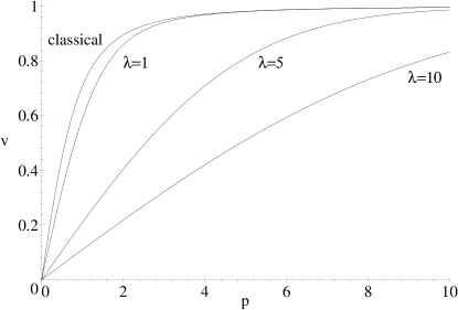
Figure 1: Dependence of the mean velocity on the mean momentum for the coherent states of a free particle with different values of the parameter $\lambda$ and for the classical (nonquantum) case. Momentum is given in $mc$ units; velocity is given in the speed of light units.

From this plot one can see that for small values of the momentum, this dependence is a nonrelativistic one but with larger mass. Indeed, writing the power series (51) with terms $n=0$ only, one can obtain the following expression (in the dimensional units):

$$\bar{v}=\frac{\bar{p}}{m^{*}},$$ (52)

where we have introduced the effective mass as follows:

$$m^{*}=\frac{m}{\frac{2}{\sqrt{\pi}}\sum\limits_{n=0}^{\infty}\lambda^{2n}C^{n}_{-1/2}\Gamma\left(n+\frac{3}{2}\right)}.$$ (53)

The difference between the standard and nonlocal theories can be verified on the expected values of observables, which contain second and higher powers of the coordinate. We consider it on the example of the dispersion of coordinate.

The second moment of the coordinate (25) contains both the standard and additional terms. The reason for this is the fact that the square of an odd operator is an even operator. Hence, the square of the dispersion for the coherent state (49) can be written (in dimensionless units) as follows:

$$\overline{\Delta q^{2}}\!=\!\frac{1}{2}-\frac{\lambda^{4}}{4\sqrt{\pi}}\!\int\limits_{-\infty}^{+\infty}\!\frac{p^{2}}{\left(1+\lambda^{2}p^{2}\right)^{2}}\exp\left(-\left(p-\sqrt{2}\alpha^{\prime\prime}\right)^{2}\right)d\!p\!.$$ (54)

In Fig. 2 we plot the dependence of the coordinate dispersion on the momentum dispersion for coherent states with different mean momenta. It should be noticed that there exists a formal violation of the uncertainty relation for all these states, especially for the large dispersion of momentum. For the very localized states, the square of dispersion even can be negative. This is a specific feature of the spin-$0$ particles, which are described by the Klein–Gordon equation. The reason for it is the indefinite metric of the Hilbert space of states. This fact makes for difficulties in the probability interpretation of these particles.

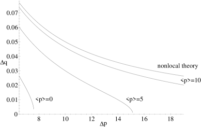
Figure 2: Dependence of the coordinate dispersion on the momentum dispersion for coherent states of a free particle with different values of the mean momentum $\left\langle p\right\rangle=\sqrt{2}\alpha^{\prime\prime}\lambda$. Dispersion of the coordinate is given in $\lambda_{c}=\hbar/mc$ units; dispersion of the momentum and mean momentum are given in $mc$ units. For comparison, the curve $\Delta q=1/(2\Delta p)$ for the coherent states in the nonlocal theory is given.

These peculiarities, which lead from the nontrivial charge structure of the coordinate operator, vanish for the strong localized states with a large mean momentum. It means that, in this case, the approximation of the nonlocal theory can be used for a description of scalar charge particles. Nevertheless, for strongly localized states with a small mean momentum these peculiarities manifest themselves.

IV Coherent states for relativistic rotator

The even part (39) of the standard annihilation operator is a deformed annihilation operator of the nonlocal theory in the case of a relativistic rotator. Hence, the corresponding coherent states are the so-called nonlinear coherent states b6 ; b7 with the $\varepsilon$ factor as a deforming function:

$$\left|\alpha,\pm\right\rangle=\mathcal{N}^{-\frac{1}{2}}\left(\left|\alpha\right|^{2}\right)\sum\limits_{n=0}^{\infty}\frac{\alpha^{n}}{\sqrt{n!}\left[\varepsilon(n)\right]!}\left|n\right\rangle\otimes\left|\pm\right\rangle.$$ (55)

Here $\left|\pm\right\rangle$ is the charge part of the quantum state. The functional factorial and the normalization factor are determined in the usual way:

$$\left[\varepsilon(n)\right]!=\left\{\begin{array}[]{ll}1&\textrm{if $n=0$}\\ \prod\limits_{k=1}^{n}\varepsilon(k)&\textrm{if $n=1,\ldots,\infty$}\end{array}\right.,$$ (56)

$$\mathcal{N}\left(\left|\alpha\right|^{2}\right)=\sum\limits_{n=0}^{\infty}\frac{\left|\alpha\right|^{2n}}{n!\left[\varepsilon^{2}(n)\right]!}.$$ (57)

The $\varepsilon$ factor is the difference between the coherent states in the standard and nonlocal theories. It results in the fact that not only the dispersions of coordinate and momentum have some peculiarities, but the expected value of the coordinate and momentum as well.

Consider briefly the properties of the function $\left[\varepsilon(n)\right]!$. From the definition (37), the $\varepsilon$ factor

$$\varepsilon(n)=1+\frac{5\lambda^{4}+3}{128\lambda^{4}}\frac{1}{n^{2}}+O\left(\frac{1}{n^{3}}\right),$$ (58)

for large $n$. Therefore the quantity $[\varepsilon(n)]!$ converges to a nonzero, finite factor as $n\rightarrow\infty$. For example, it is possible to find nonzero numbers $a$ and $b$ such that

$$\exp\left(\frac{a}{n^{2}}\right)<\varepsilon\left(n\right)<\exp\left(\frac{b}{n^{2}}\right)$$ (59)

holds for all $n>0$. In this case

$$\exp\left(\frac{\pi^{2}a}{6}\right)<\lim_{n\rightarrow\infty}\left[\varepsilon(n)\right]!<\exp\left(\frac{\pi^{2}b}{6}\right).$$ (60)

Hence this case has the property that the terms with the large $n$ are effectively of the canonical form where $\sqrt{n!}$ is the controlling factor. From this fact we would be certainly inclined to believe that $\varepsilon$ factor influences on the particle behavior are very low.

Consider this fact on the example of the expected values of the coordinate and momentum time evolution. The Heisenberg equation in the representation of the nonlocal theory has the following form:

$$\partial_{t}[\hat{a}]=-\frac{i}{\hbar}\tau_{3}\left(E\left(\hat{n}+1\right)-E\left(\hat{n}\right)\right)[\hat{a}],$$ (61)

$$\partial_{t}\{\hat{a}\}=\frac{i}{\hbar}\tau_{3}\left(E\left(\hat{n}+1\right)+E\left(\hat{n}\right)\right)\{\hat{a}\},$$ (62)

where $[\hat{a}]$ and $\{\hat{a}\}$ are the even and odd parts of the standard annihilation operator. Their solution can be written as follows:

$$[\hat{a}]\left(t\right)=\exp\left(-\frac{i}{\hbar}\tau_{3}\left(E\left(\hat{n}+1\right)-E\left(\hat{n}\right)\right)t\right)[\hat{a}],$$ (63)

$$\{\hat{a}\}\left(t\right)=\exp\left(\frac{i}{\hbar}\tau_{3}\left(E\left(\hat{n}+1\right)+E\left(\hat{n}\right)\right)t\right)\{\hat{a}\}.$$ (64)

The expected value of this operator in the coherent state (55) is

$$\bar{a}\!\left(t\right)\!=\!\pm\!\alpha\!\mathcal{N}^{-1}\!\left(\!\left|\alpha\right|^{2}\!\right)\!\sum\limits_{n=0}^{\infty}\!\frac{\left|\alpha\right|^{2n}}{n\!!\!\left[\!\varepsilon^{2}(n)\!\right]\!!}\!\exp\!\left(\!\mp\!\frac{i}{\hbar}\!\left(\!E\!\left(\!n\!+\!1\!\right)\!-\!E\!\left(\!n\!\right)\!\right)\!t\!\right)\!.$$ (65)

In the first relativistic correction, the dependence on the $\varepsilon$ factor vanishes and this expected value can be calculated analytically b13 :

$$\bar{a}\left(t\right) = \pm\!\alpha\exp\left(-2\left|\alpha\right|^{2}\sin^{2}\left(\frac{\lambda^{2}\omega t}{2}\right)\right)$$ (66)

$$\times \!\exp\left(\mp i\left[\left(1-\lambda^{2}\right)\omega t-\left|\alpha\right|^{2}\sin\left(\lambda^{2}\omega t\right)\right]\right)\!.$$

Along with the cyclotron frequency, there exists the low frequency

$$\Omega=\lambda^{2}\omega<\omega,$$ (67)

that modulates the rotational motion. However, due to the bremsstrahlung, it can be regarded as an additional damping rather than a low frequency modulation in the real physical systems.

In Fig. 3 we plot the results of numerical calculations for the time evolution of the mean gyration radius. First of all it should be noticed that dependence on the $\varepsilon$-factor is very small. Only in the case where $\lambda$ is large enough and the initial radius small, one can distinguish between the standard and nonlocal theories. This difference is very insignificant. Also, we note that the low-frequency is intrinsic to all cases. However, in real physical systems this effect should be very suppressed by the bremsstrahlung.

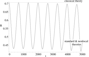
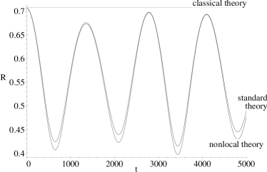
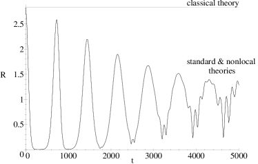
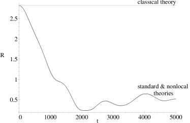
(a) (b) (c) (d)

Figure 3: The time evolution of the mean gyration radius of a relativistic rotator in classical and quantum relativistic (standard and nonlocal) theories. The radius is given in the dimensionless units; time is given in $1/\omega$ units. (a) $\lambda=0.1$, $\overline{q}=0.5$, $\overline{p}=0.5$. This case can be calculated analytically. (b) $\lambda=50$, $\overline{q}=0.5$, $\overline{p}=0.5$. In this case one can distinguish between the standard and nonlocal theories. (c) $\lambda=0.1$, $\overline{q}=2$, $\overline{p}=2$. (d) $\lambda=50$, $\overline{q}=2$, $\overline{p}=2$. In the all cases (not only with small $\lambda$) the low-frequency harmonic exists.

Similar to the case of a free particle, the more significant difference between the standard and nonlocal theories can be exhibited in the second moments. Consider the square of the gyration radius

$$\hat{R}^{2}=2\hat{n}+1.$$ (68)

Note that this observable is an integral of motion. Then, one can find the dispersion of the gyration radius as follows:

$$\overline{\Delta R^{2}}=1-\overline{R}^{2}\left(1-\mathcal{N}^{-1}\left(\overline{R}^{2}/2\right)\sum\limits_{n=0}^{\infty}\frac{\overline{R}^{2n}}{2^{n}n!\left[\varepsilon^{2}(n+1)\right]!}\right),$$ (69)

where $\overline{R}^{2}=2\left|\alpha\right|^{2}$.

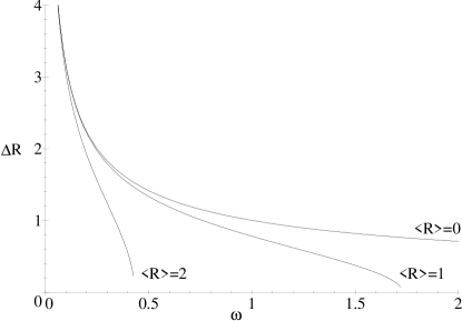
Figure 4: Dependence of the gyration radius dispersion on the cyclotron frequency for coherent states of a relativistic rotator with different values of the mean gyration radius $\left\langle R\right\rangle$. The cyclotron frequency is given in $mc^{2}/\hbar$ units; the dispersion of gyration radius and mean radius are given in $\lambda_{c}=\hbar/mc$ units. Case $\left\langle R\right\rangle=0$ coincides with a curve for a coherent state in the nonlocal theory.

The results of the numerical calculations for the dependence of the gyration radius dispersion on the cyclotron frequency are given in the Fig. 4. Unlike the case of a free particle, the peculiarities resulting from the nontrivial charge structure of the coordinate and momentum operators are more evident for the coherent states with large parameter $\alpha$ (mean gyration radius). The case of $\alpha=0$ corresponds to the eigenstate of the Hamiltonian with $n=0$. All peculiarities are absent here.

V Coherent states for a particle in a constant homogeneous magnetic field

The consideration of a particle in a constant homogeneous magnetic field combines the two previous cases. However, it is impossible to construct coherent states that satisfy our conditions for both the translational and rotational degrees of freedom simultaneously, because the even parts of the corresponding annihilation operators do not commutate with each other (see Eq. (47)). Therefore we will define coherent states for each degree of freedom separately.

The coherent state for the translational motion has the following form:

$$\left|n,\alpha_{z},\pm\right\rangle=\left|n\right\rangle\otimes\left|\alpha_{z}\right\rangle\otimes\left|\pm\right\rangle,$$ (70)

where $\left|\alpha_{z}\right\rangle$ is the standard coherent state for the $z$ axis and $\left|n\right\rangle$ is the eigenstate of the rotator. The coherent state for the rotational motion can be written as follows:

$$\left|\alpha_{r},p_{z},\pm\right\rangle\!=\!\mathcal{N}^{-\frac{1}{2}}\left(\!\left|\alpha_{r}\right|^{2},\!p_{z}\!\right)\!\sum\limits_{n=0}^{\infty}\!\frac{\alpha_{r}^{n}}{\sqrt{n!}\!\left[\!\varepsilon(\!n,p_{z}\!)\!\right]\!!}\!\left|n\right\rangle\!\otimes\!\left|p_{z}\right\rangle\!\otimes\!\left|\pm\right\rangle\!,$$ (71)

where $\left|p_{z}\right\rangle$ is the eigenstate of the $z$ component of momentum and the normalization factor is determined in the form:

$$\mathcal{N}\left(\left|\alpha_{r}\right|^{2},p_{z}\right)=\sum\limits_{n=0}^{\infty}\frac{\left|\alpha_{r}\right|^{2n}}{n!\left[\varepsilon^{2}(n,p_{z})\right]!}.$$ (72)

It should be noticed that in the present form the coherent state (71) includes an eigenstate of the $z$ component of momentum. Hence, it is normalized on $\delta$ function

$$\left\langle\pm,p^{\prime}_{z},\alpha_{r}|\alpha_{r},p_{z},\pm\right\rangle=\pm\delta\left(p_{z}-p^{\prime}_{z}\right).$$ (73)

Generally speaking, the states (70) and (71) are direct products of coherent states on the one degree of freedom and part of the Hamiltonian eigenstates on another one. These states can be redefined in such a way to be the coherent states for both degrees of freedom. However, they will not satisfy condition 1 from the Introduction for one of them.

Summing the states (70) on $n$ with $e^{-\frac{\left|\alpha_{r}\right|^{2}}{2}}\alpha_{r}^{n}/\sqrt{n!}$, one can obtain the coherent states of the nonlocal theory presented in b12 ,

$$\left|\alpha_{r},\alpha_{z},\pm\right\rangle=\left|\alpha_{r}\right\rangle\otimes\left|\alpha_{z}\right\rangle\otimes\left|\pm\right\rangle,$$ (74)

where $\left|\alpha_{r}\right\rangle$ is a standard coherent state for the rotational degree of freedom. For the rotational motion these states do not satisfy condition 1 from the Introduction.

Now, integrating the states (71) with $\Psi_{\alpha_{z}}\left(p_{z}\right)$ (the standard coherent states in the momentum representation), one can obtain the following coherent states:

$$\left|\alpha_{r},\alpha_{z},\pm\right\rangle$$

$$\!=\sum\limits_{n=0}^{\infty}\!\int\limits_{-\infty}^{\infty}\!d \!p_{z}\! \!\Psi_{\alpha_{z}}\!\left(\!p_{z}\!\right)\!\mathcal{N}\!^{-\frac{1}{2}}\!\left(\!\left|\!\alpha_{r}\!\right|^{2}\!,\!p_{z}\!\right)\!\frac{\alpha_{r}^{n}}{\sqrt{n!}\!\left[\!\varepsilon\!(\!n\!,\!p_{z}\!)\!\right]\!!}\!\left|\!n\!\right\rangle\!\otimes\!\left|\!p_{z}\!\right\rangle\!\otimes\!\left|\!\pm\!\right\rangle\!.$$

These coherent states do not satisfy condition 1 for the translational motion along the field b13 . Nevertheless, they are eigenstates of the even part of the annihilation operator (46), and describe the rotational motion taking into account a finite localization along the $z$ axis.

In the approximation of the nonlocal theory and for the first relativistic correction of the standard theory, the states (74) and (LABEL:f65) are the same. Hence, one can find the time evolution of the first moments of the rotational motion in this case as follows:

$$\overline{a_{r}}\left(t\right) = \pm\alpha_{r}\frac{1}{\sqrt[4]{1+\frac{\lambda_{z}^{4}\omega^{2}t^{2}}{4}}}\exp\left(-2\left|\alpha_{r}\right|^{2}\sin^{2}\left(\frac{\lambda_{r}^{2}\omega t}{2}\right)-\frac{\alpha_{z}^{\prime\prime 2}\lambda_{z}^{4}\omega^{2}t^{2}}{2+\frac{\lambda_{z}^{4}\omega^{2}t^{2}}{2}}\right)$$ (76)

$$\times \exp\left(\mp i\left[\left(1-\lambda_{r}^{2}\right)\omega t-\left|\alpha_{r}\right|^{2}\sin\left(\lambda_{r}^{2}\omega t\right)-\frac{\alpha_{z}^{\prime\prime 2}\lambda_{z}^{2}\omega^{2}t^{2}}{1+\frac{\lambda_{z}^{4}\omega^{2}t^{2}}{4}}+\frac{1}{2}\arctan\left(\frac{\lambda_{z}^{4}\omega^{2}t^{2}}{4}\right)\right]\right).$$

Therefore, from the comparison of this equation and Eq. (66), one can conclude that the localization along the $z$ axis leads to the peculiarities of the rotational motion for the time

$$t>\frac{1}{\lambda_{z}\omega}.$$ (77)

For the mean velocity of the translational motion along $z$ axis we have the following:

$$\bar{v}_{z}=\overline{p}_{z}\left[\frac{1}{m^{*}}-\frac{\hbar\omega}{m^{2}c^{2}}\left(\left|\alpha_{r}\right|^{2}+\frac{1}{2}\right)\right].$$ (78)

The second term in this equation is the same in the classical (nonquantum) theory. Hence, the peculiarities of the translational motion result only from the localization along this degree of freedom in such approximation.

VI Coherent states in the Wigner representation

The localization peculiarities, which have been described in the preceding sections, can be illustrated by means of the relativistic Wigner function for charge-invariant observables b17 ; b18 . The nontrivial charge structure of the coordinate and momentum operators is taken into account in this representation.

Utilizing the definition of the Wigner function from b17 , one can obtain for the coherent state of a free particle (49) (for determination, we consider only positive charge):

$$W_{[+],\alpha}\!(p,q)\!=\!\frac{1}{\pi^{3/2}}\!\exp\!\left(\!-\left(p-\sqrt{2}\alpha^{\prime\prime}\right)^{2}\!\right)$$

$$\!\times\!\int\limits_{-\infty}^{+\infty}\!\left(\!\frac{1\!+\!\lambda^{2}\!\left(\!p\!+\!x\!\right)^{2}}{1\!+\!\lambda^{2}\!\left(\!p\!-\!x\!\right)^{2}}\!\right)^{1/4}\!\exp\!\left(\!-x^{2}\!\right)\!\cos\!\left(\!2\!\left(\!q\!-\!\sqrt{2}\alpha^{\prime}\!\right)\!x\!\right)\!d\!x\!.$$

(79)

Due to the negative square of the coordinate dispersion for strong localized states, there exists the supposition that such states are impossible. In Fig. 5 we plot the Wigner function for such a state. One can see that negative square dispersion is the consequence of the “vacuum perturbations” on the size near the Compton wavelength in the domain around the origin of coordinates. However, this state is localized very well. The perturbations do not influence the expected values of observables when the mean moment is away from $0$.

The Wigner function for the coherent state (55) of the relativistic rotator can be written as the following expression b18 :

$$W_{[+],\alpha}(p,q)=\frac{1}{\pi}\exp\left(-q^{2}-p^{2}\right)\exp\left(-\left|\alpha\right|^{2}\right)$$

$$\times\!\sum\limits_{m,n=0}^{\infty}\!\frac{\varepsilon(m,n)}{[\varepsilon(m)]![\varepsilon(n)]!}\left(\sqrt{2}(q+ip)\overline{\alpha}\right)^{m}\!\left(\sqrt{2}(q-ip)\alpha\right)^{n}$$

$$\times\!\sum\limits_{k=0}^{\min(m,n)}\!\frac{1}{(-2(q^{2}+p^{2}))^{k}(m-k)!(n-k)!k!},$$ (80)

where $\varepsilon(n,m)$ is the $\varepsilon$ factor of two variables:

$$\varepsilon(n,m)=\frac{{E(n)+E(m)}}{{2\sqrt{E(n)E(m)}}}.$$ (81)

The plot of this Wigner function is presented in Fig. 6. Unlike the case of a free particle, “vacuum perturbations” increase as $\alpha\rightarrow\infty$ here. They may be seen as the large negative domain near the origin of coordinates.

VII Resolution of unity

The resolution of unity is one of the key properties of the coherent states. In this section we consider it for the relativistic case presented here. Note that for a free particle, where these states are the standard coherent states, the measure is determined by Eq. (5). Hence we consider more complicated cases of a relativistic rotator.

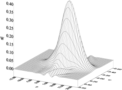
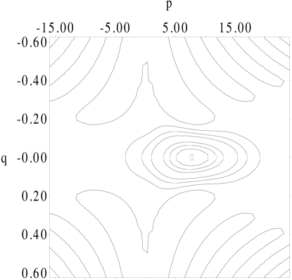
(a) (b)

Figure 5: The Wigner function (a) and its contours (b) for the coherent state of a free particle. The ratio of the Compton wavelength and character wave-packet length is $\lambda=8$. The mean momentum is $8mc$. In this plot momentum is given in $mc$ and the coordinate in $\lambda_{c}=\hbar/mc$ units.

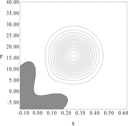
Figure 6: The contours of the Wigner function for the coherent state of a relativistic rotator. The ratio of the Compton wavelength and oscillator length is $\lambda=8$. The mean momentum and coordinate are $16mc$ and $1/4\lambda_{c}$ respectively. The coordinate is given in $\lambda_{c}$ units; the momentum is given in $mc$ units (absolute). The domain of the negative values is marked in black.

It is known (see, for example, b7 ) that the integral measure in Eq. (4) for the coherent states (55) can be written in the form

$$d\mu\left(\alpha\right)=\mathcal{N}\left(\left|\alpha\right|^{2}\right)\mathcal{W}\left(\left|\alpha\right|^{2}\right)\frac{d\alpha^{\prime}d\alpha^{\prime\prime}}{\pi},$$ (82)

where the weight function $\mathcal{W}\left(x\right)$ is determined from the following integral equation:

$$\int\limits_{0}^{+\infty}x^{n}\mathcal{W}\left(x\right)dx=n!\left[\varepsilon^{2}(n)\right]!.$$ (83)

The resolution of unity for the states given in Eq. (LABEL:f65) is rather more complicated than usual. We do not develop that resolution of unity in this paper, but we hope to return to this question in a subsequent article.

VIII Conclusions

In this paper we have considered the relativistic coherent state taking into account the fact that eigenfunctions of the standard coordinate and momentum operators have both charge components. However, the coherent states presented here contain only one charge component and in that case the real and imaginary parts of the parameter $\alpha$ are uniquely related to the expected values of the standard coordinate and momentum. We obtained this result through the determination of the coherent states as eigenstates of the even part of the annihilation operator. Indeed, these coherent states do not satisfy the property of temporal stability, and time evolution of the mean position and momentum is, generally speaking, a nontrivial question.

In order to obtain the even part of the annihilation operator, one needs to change the standard coordinate to the Newton–Wigner position for the case of a free particle. Hence, the average coordinate and momentum have no peculiarities here. Nevertheless, the second moments (dispersion) differ from ones in the nonlocal theory and nonrelativistic quantum mechanics, especially for very localized states.

Both the coordinate and momentum have a nontrivial charge structure in the case of a relativistic rotator. Furthermore, the even parts of these operators do not satisfy the commutation relations of the usual Heisenberg–Weyl algebra. “Mean positions” have the property of a deformed algebra in this case. Therefore, the coherent states have some peculiarities and are the so-called nonlinear coherent states. This deformation is the consequence of the interaction with the vacuum. In fact it is very small, and leads to insignificant differences for the mean trajectory, but it leads to essential peculiarities for the second moments.

A specific peculiarity for the case of a particle in a constant homogeneous magnetic field is the fact that the “mean positions” of the translational and rotational motions do not commutate with each other. Hence, we cannot construct the coherent states that satisfy our conditions here. However, we have presented states, which first of all, satisfy condition (2) from the Introduction and, second, satisfy condition (1) only for one degree of freedom.

Furthermore, it should be noticed that relativistic quantum motion has other peculiarities, which are not consequences of the nontrivial charge structure of the coordinate and momentum operators. These properties result from the Ehrenfest theorem because the relativistic Hamiltonian is effectively nonquadratic. For a free particle it leads to the effective increase of the mass (effective mass can be presented here). For the rotational motion it leads to the low-frequency fluctuations of the gyration radius.

- (1) E. Schrödinger, Naturwissenschaften 14, 664 (1926).
- (2) J.R. Klauder and B.-S. Skagerstam, Coherent States: Applications in Physics and Mathematical Physics (World Scientific, Singapore, 1985).
- (3) J.R. Klauder, J. Math. Phys. 4, 1058 (1963).
- (4) J.P. Gazeau and J.R. Klauder, J. Phys. A 32, 123 (1999).
- (5) J.-P. Antoine, J.-P. Gazeau, P. Monceau, J.R. Klauder, and K.A. Penson, J. Math. Phys. 42, 2349 (2001).
- (6) R.L. de Matos Filho and W. Vogel, Phys. Rev. A 54, 4560 (1996).
- (7) V.I. Man’ko, G. Marmo, E.C.G. Sudarshan, and F. Zaccaria, Phys. Scr. 55, 528 (1997).
- (8) T.D. Newton and E.P. Wigner, Rev. Mod. Phys. 21, 400 (1949).
- (9) L.L. Foldy and S.A. Wouthuysen, Phys. Rev. 78, 29 (1950).
- (10) H. Feshbach and F. Villars, Rev. Mod. Phys. 30, 24 (1958).
- (11) E.P. Wigner, Z. Phys. 133, 101 (1952); G.C. Wick, A.S. Wightman and E.P. Wigner, Phys. Rev. 88, 101 (1952).
- (12) I.A. Malkin and V.I. Man’ko, Sov. Phys. JETP 28, 527 (1969).
- (13) B.I. Lev, A.A. Semenov and C.V. Usenko, Phys. Let. A. 230, 261 (1997). In this reference the mistaken statement that states (LABEL:f65) are eigenstates of the both annihilation operators, has been made. However, it does not influence the results of that work because the effects, related to the factor, have not been considered there.
- (14) M.H. Johnson and B.A. Lippmann, Phys. Rev. 76, 828 (1949).
- (15) A.J. Bracken and G.F. Melloy, J. Phys. A 32, 6127 (1999).
- (16) S.R. de Groot and L.G. Suttorp, Fundations of Electrodynamics (North-Holland, Amsterdam, 1972).
- (17) H.-J. Briegel, B.-G. Englert, M. Michaelis, and G. Süssmann, Z. Naturforsch. A: Phys. Sci. 46, 925 (1991); H.-J. Briegel, B.-G. Englert, and G. Süssmann, ibid. 46, 933 (1991).
- (18) H.S. Snyder , Phys. Rev. 71, 38 (1947).
- (19) G.V. Dunne, R. Jackiw, and C.A. Trugenberger, Phys. Rev. D 41, 661 (1990).
- (20) B.I. Lev, A.A. Semenov, and C.V. Usenko, J. Phys. A 34, 4323 (2001); B.I. Lev, A.A. Semenov, and C.V. Usenko, e-print quant-ph/0102095.
- (21) B.I. Lev, A.A. Semenov, and C.V. Usenko, J. Rus. Las. Res. 23, 347 (2002); B.I. Lev, A.A. Semenov, and C.V. Usenko, e-print quant-ph/0112146.