Quantum Trajectories for Realistic Photodetection I: General Formalism

Abstract

Quantum trajectories describe the stochastic evolution of an open quantum system conditioned on continuous monitoring of its output, such as by an ideal photodetector. In practice an experimenter has access to an output filtered through various electronic devices, rather than the microscopic states of the detector. This introduces several imperfections into the measurement process, of which only inefficiency has previously been incorporated into quantum trajectory theory. However, all electronic devices have finite bandwidths, and the consequent delay in conveying the output signal to the observer implies that the evolution of the conditional state of the quantum system must be non-Markovian. We present a general method of describing this evolution and apply it to avalanche photodiodes (APDs) and to photoreceivers. We include the effects of efficiency, dead time, bandwidth, electronic noise, and dark counts. The essential idea is to treat the quantum system and classical detector jointly, and to average over the latter to obtain the conditional quantum state. The significance of our theory is that quantum trajectories for realistic detection are necessary for sophisticated approaches to quantum feedback, and our approach could be applied in many areas of physics.

I Introduction

I.1 Measurement in Quantum Mechanics

To obtain information about a system of interest a measurement has to be made. In experiments that probe the quantum nature of our world, the system itself is, in general, necessarily affected by the act of measurement. For experiments involving continuous monitoring, traditional (projective) measurement theory as axiomatized by von Neumann Von32 is inadequate as a description. Such measurements would prevent any interesting evolution occurring, because of the quantum Zeno effect zeno1 . To avoid this, a generalized quantum theory of measurement must be used Dav76 ; Kra83 . Generalized quantum measurements can be derived by considering projective measurements on a second system interacting with the system of interest. Often the second system has a clear physical interpretation. For example, in quantum optics a bath (continuum) of electromagnetic field modes plays this role and the quantum system is said to be open.

If the system is weakly coupled to its bath and the dynamics are such that information concerning the system is spread throughout the many degrees of freedom of the bath, then a Markovian evolution equation for the system alone may be obtained. This equation is known as a master equation (ME). If, in addition, the bath is being measured then a stochastic master equation (SME) for the conditioned state of the system can be found. This is termed a quantum trajectory Car93b . The relation of the ME to quantum trajectories is that the former results from summing all possible trajectories, weighted by their probability of occurrence. Thus, the ME represents average evolution and gives the evolution of the state of the system when the environment is not monitored. A quantum trajectory (which is said to ‘unravel’ the master equation) gives the evolution of the state of the system conditioned on the results of monitoring the environment. A quantum trajectory is necessarily stochastic, and can be jumpy Car93b ; DalCasMol92 ; GarParZol92 or diffusive Bel88 ; BelSta92 ; Bar90 ; Bar93 ; Car93b ; WisMil93c , depending on the nature of the measurement.

I.2 Realistic Quantum Trajectories

In experiments performed in the laboratory, a detector mediates between the detector input (for example, the electromagnetic field emitted by a fluorescent quantum system) and the experimenter. Realistic detectors are not perfect. Information is lost in the conversion of the quantum field to a signal that the observer can use. This loss may occur at the front end of the detector (characterized by an inefficiency), in the circuit containing the detector (described by a response time and electronic noise) or at the circuit output (electronic output noise). In order to obtain a true quantum trajectory for the experiment, the observer must condition the state of the quantum system on results that are available in the laboratory rather than on the microscopic absorption events considered previously in quantum trajectories.

Realistic quantum trajectories of this sort cannot be encompassed within the standard formalism of Refs. Dav76 ; Kra83 , except for inefficiency WisMil93a . This is because the electrical circuit, which filters the measured output of the quantum system, causes a statistical delay in the observer obtaining information about the system. Thus the conditioned evolution of the quantum system alone is non-Markovian. A method for treating this was first proposed by us and Mabuchi WarWisMab01 , in which the quantum system is embedded within a supersystem that also contains the state of the detector. If the set of (classical) detector states is $\mathbb{S}$, then the supersystem is described by the set $\{\rho_{s}:s\in\mathbb{S}\}$. Here ${\rm Tr}[\rho_{s}]$ is the probability that the apparatus is in state $s$, and $\rho_{s}/{\rm Tr}[\rho_{s}]$ is the system state given this event. The supersystem state, $\left\{{\rho_{s}}\right\}$, obeys a Markovian evolution equation. The detector states are classical in the sense that it is not necessary to consider superpositions between them.

In this paper we consider in detail two sorts of realistic detectors, an avalanche photodiode in geiger mode (a photon counter) and a photoreceiver (for homodyne detection). The detector states in the former case are discrete (we use three states) and in the latter continuous (although discretization is necessary for numerical simulation). For the photon counter, this model allows us to include the effects of detection efficiency, dark counts, response (or rise) time and dead time. For homodyne detection using a photoreceiver we investigate detector efficiency, output Johnson noise (which adds onto the measurement result linearly) and detector bandwidth. (Of course, this bandwidth relates not to the range of frequencies (colours) of light to which the detector will respond, but to the characteristic time it takes for the absorption of light by the detector to generate a response in the detector output.)

Before passing onto our method of derivation of realistic quantum trajectories, it is worth mentioning that a three-level model for a photon counter including many of the above effects has been considered by Gardiner Gar91 . However this theory is based upon quantum Langevin equations rather than quantum trajectories, and does not allow one to determine the system state conditioned on the experimenter’s knowledge.

I.3 Derivation of Realistic Quantum Trajectories

The derivation of realistic quantum trajectories consists of a number of well defined steps, that are schematically illustrated in Fig. 1. These can be understood by considering the subsystems that make up the supersystem, namely the quantum system and the detector.

Figure 1: Schematic diagram for the method that we use to derive realistic quantum trajectories. It should be noted that some of the steps shown above can be performed in a different order. This flexibility is useful for keeping the derivation of realistic quantum trajectories as simple as possible. The following abbreviations have been used: stochastic master equation (SME), stochastic differential equation (SDE), stochastic differential Chapman-Kolmogorov equation (SDCKE), Kushner-Stratonovich equation (KSE) and superoperator Kushner-Stratonovich equation (SKSE). Hexagons, rectangles and circles indicate bodies of knowledge, equations and procedures, respectively. See text for further details.

The basic philosophy that we adopt at the start of the derivation is that in principle all of the microscopic states of the detector could be monitored, without altering the quantum trajectory of the system. Essentially this is because the detector states consist of distinct configurations of an enormous number of particles. These particles are constantly interacting with their environment, thus making coherences between detector states unimportant. Thus in principle it is possible for an experimenter to have sufficient information to unravel the evolution of the system by a conventional stochastic master equation (SME). In practice, an experimenter has access to far less knowledge. This loss of knowledge is due to classical uncertainties introduced by the detector.

To describe the detector we consider some property of it that can be related to the output that the observer monitors. For example, in the case of homodyne detection the charge across one of the capacitors in the circuit represents the detector state. By considering all of the dynamic influences upon this circuit variable we formulate an evolution equation for it that is stochastic in general. Since finally we will not know the stochastic inputs, we transform this into a stochastic differential Chapman-Kolmogorov equation (SDCKE) that follows the probability of the various states being occupied. We use this terminology to indicate a generalization of the deterministic differential Chapman-Kolmogorov equation discussed in Gar85 .

The realistic measurement results available to the observer give information about the detector state, without necessarily revealing it fully. Based on the result and the a priori (initial) probability distribution for the detector state, the best estimate of the updated state (the a posteriori distribution) is found. This is done via a Bayesian analysis BayesBook . The resulting equation for the the probability distribution is, for the case of Gaussian white noise, usually referred to as a Kushner-Stratonovich equation (KSE) KSBook . For convenience we will use this terminology even in the case of point-process noise.

Note that normally a KSE would also contain that unconditioned (deterministic) evolution due to the system dynamics. Since these dynamics are stochastic at this stage of the derivation (they are contained in the SDCKE), we do not include them in the KSE for the detector state. Note also that the SME, despite its name (introduced in Ref. WisMil93a ), is conceptually closer to the KSE than to the SDCKE: the stochasticity in both the KSE and the SME is solely due to measurement noise, and the stochastic terms are nonlinear in both cases. In fact, the SME can justifiably be called a quantum KSE Dohe2000 .

The evolution of the SME, the SDCKE and the KSE are combined to give the joint stochastic equations governing the evolution of the supersystem. Up until this stage all the stochastic influences on the supersystem are still present. To link the evolution of the system with that of the detector this is necessary. Now, however, we average over processes that a realistic observer cannot monitor. This leaves only the stochasticity associated with the measurement and our derivation of the realistic quantum trajectory is then complete. We term this final stochastic trajectory for the supersystem a superoperator Kushner-Stratonovich equation (SKSE). Obviously the reader will gain much greater insight into this process by following the examples provided in the later sections.

I.4 Importance of Realistic Quantum Trajectories

Thus far, the main practical utility of quantum trajectory theory has been in improving the computational efficiency of simulations used to compare models with experimental data. For this purpose, the introduction of realistic quantum trajectories could only hinder simulations. However, quantum trajectory theory is now gaining increasing importance as the quantum generalization of Kalman filtering, which provides essential signal-processing methods in classical estimation, communication, and control engineering. Quantum trajectory theory should in principle play the same pivotal role for emerging quantum analogs of these technologies Gamb01 ; Cira97 ; Dohe99b . Before this can happen it is essential that the theory be extended to account for the imperfections of realistic measurement devices. Non-ideal detector dynamics can dramatically affect the proper inference from measured signals to the conditional quantum state of an observed system, as we will show.

I.5 Overview of this Paper

As stated above, the main thrust of this paper is to derive in detail the realistic quantum trajectories for photon counting and homodyne photodetection introduced in Ref. WarWisMab01 . In Sec. II, we first briefly give the theory of classical trajectories and measurement, which is important for obtaining SDCKEs and KSEs for the detector state. A discussion of non-realistic (that is, ideal) quantum trajectories follows this, which allows the SMEs for the quantum system to be found.

In Secs. III and IV, realistic quantum trajectories are derived for photon counters and photoreceivers respectively. Both of these derivations are based on the procedure outlined in Sec. I.3. For the photon counter, we finally idealize the measurement process to show that our equations reduce to those associated with perfect detection (traditional quantum trajectories). An important and non-trivial consideration in the case of the photoreceiver is the bandwidth of the device. As the photoreceiver circuit adds electronic noise, a calculation of this bandwidth based on just the resistance-capacitance ($RC$) time constant of the circuit does not yield the correct answer. As a final point we consider the effect of letting the $RC$ time constant go to zero but still maintaining the presence of the electronic noise which obscures the input signal. We conclude with a summary of our results and discussion of future directions in Sec. V. A numerical exploration of our theory is given in the following paper WarWis02b .

II Stochastic Equations

As discussed in Sec. I.3, there are three types of stochastic equations that go into making a realistic quantum trajectory. In this section we examine the general theory for each.

II.1 Stochastic Differential Chapman-Kolmogorov Equation

A typical Langevin equation or stochastic differential equation (SDE) for a classical random variable $X$ can be written as

$$dX=a(X)dt+\sqrt{D}\,dW(t)+edN(t).$$ (1)

Here $a(X)$ is an arbitrary function of $X$, and $dW(t)$ and $dN(t)$ are stochastic increments. The point process $dN(t)$ is either zero or one, and has an infinitesimal mean which is a positive function of $X$, say $g(X)dt$. The Wiener increment $dW(t)$ is related to Gaussian white noise $\xi(t)$ by $dW(t)=\xi(t)dt$. Gaussian white noise has statistics of Gar85

$${\rm E}[\xi(t)]=0,\;\;{\rm E}[\xi(t)\xi(t^{\prime})]=\delta(t-t^{\prime}).$$ (2)

Here the roman font E denotes expectation value. By writing the SDE in the form of Eq. (1) we imply that the equation is to be interpreted in the Itô Gar85 or explicit Wis94 sense. This means, for example, that the expected value of $dX$ may be found by replacing $dN$ and $dW$ by their expected value. This is not true for the implicit Wis94 or Stratonovich Gar85 form. By the same token, the chain rule of standard calculus does not apply in general to the Itô form, whereas it does for the Stratonovich form.

Langevin equations are appropriate for situations in which the stochastic increment is known, thus allowing $X$ to be tracked. Often it is relatively easy to turn the physics of a problem into a Langevin equation. An example of this is a noisy electrical circuit. The analysis of such circuits is well understood and is based on simple principles such as Kirchhoff’s laws.

In this paper, Langevin equations are first found on the presumption that the stochastic increment is known. In reality, however, this is not the case and we cannot track the variable $X$ perfectly. For this reason it is necessary to turn the Langevin equation into an equation describing the evolution of the probability distribution for $X$, which is written as $P(x)$. Note that the transformations that we perform actually maintain the stochastic nature of this evolution equation, as the averaging over unobserved processes is done at a later stage. This is necessary because the noise in the equation for $P(x)$ may also appear in other parts of the overall derivation. Before this final averaging is done, the stochastic equation for $P(x)$, would preserve a Dirac $\delta$-function as a solution. We now do this for Eq. (1), as an aid the reader.

If $X$ is known at time $t$, then at that time $P(x)=\delta(x-X)$. This then evolves according to

$$d\delta(x-X) = \delta(x-X-dX)-\delta(x-X)$$ (4)

$$= \delta[x-X-a(X)dt-\sqrt{D}\,dW(t)-edN(t)]$$

$${-}\,\delta(x-X).$$

We can treat the diffusion and jump noise in a unified fashion by constructing a Taylor series of Eq. (4) to all orders of the first term on the right-hand side (RHS):

$$d\delta(x-X) = \left(\exp\left\{\frac{\partial}{\partial x}\left[-a(X)dt-\sqrt{D}\,dW(t)\right.\right.\right.$$ (5)

$$\left.\left.\phantom{\frac{1}{1}}\left.\phantom{\sqrt{1}\,}-edN(t)\right]\right\}-1\right)\delta(x-X).$$

We now expand the exponential to all orders and use the Itô rules $dN^{2}=dN$, $dW^{2}=dt$, with all other products being zero. This gives

$$d\delta(x-X) = \left\{-\frac{\partial}{\partial x}\left[a(X)dt+\sqrt{D}\,dW(t)\right]\right.$$

$$+\left.\phantom{\frac{1}{1}}\frac{D}{2}\frac{\partial^{2}}{\partial x^{2}}dt\right\}\delta(x-X)$$

$${+}\,dN(t)\left[\delta(x-X-e)-\delta(x-X)\right]$$

Using the delta function to change $a(X)$ to $a(x)$ and then averaging over the random variable $X$ gives the Itô equation for the probability $P(x)\equiv{\rm E}[\delta(x-X)]$,

$$dP(x) = \left\{\frac{\partial}{\partial x}\left[-a(x)dt-\sqrt{D}\,dW(t)\right]+\frac{D}{2}\frac{\partial^{2}}{\partial x^{2}}dt\right\}$$ (7)

$${\times}\,P(x)+dN(t)\left[P(x-e)-P(x)\right].$$

The first ($dt$) term is deterministic drift, the second ($dW$) is stochastic drift, the third ($dt$) is diffusion and the last ($dN$) is the jump term. We refer to this equation as a stochastic differential Chapman-Kolmogorov equation (SDCKE). If there were no jump term, then we would have a stochastic Fokker-Planck equation.

If averages over $dW(t)$ and $dN(t)$ are taken then we have a standard (deterministic) differential Chapman-Kolmogorov equation

$$\frac{\partial}{\partial t}P(x) = \left\{-\frac{\partial}{\partial x}a(x)+\frac{D}{2}\frac{\partial^{2}}{\partial x^{2}}\right\}P(x)$$ (8)

$${+}\,g(x-e)P(x-e)-g(x)P(x),$$

where $g(x)$ enters from the definition E$\left[{dN(t)f(X)}\right]={\rm E}[g(X)f(X)]$.

II.2 Kushner-Stratonovich Equation

From the point of view of measurement, it useful to consider the state of a classical system to be defined by the probability distribution on state space. This is the space of all relevant physical quantities, called state variables. In this paper the classical system will be a detector and the associated electrical circuit. Only one variable is necessary to describe it so we can think of the distribution $P(x)$ that was introduced in the previous section as representing the state.

As the state of the system summarizes the observer’s knowledge it is logical that the state will change on the basis of measurement upon the system. From the a priori state $P(x)$ of the system and the result $r$ of measurement, the a posteriori state $P(x|r)$ can be found using Bayesian inference BayesBook

$$P(x|r)=\frac{P(r|x)P(x)}{P(r)}.$$ (9)

Here $P(x|r)$ reads as ‘the probability of $x$ given $r$’. The division by $P(r)$ is for normalization purposes, where

$$P(r)=\int dx\,P(r|x)P(x).$$ (10)

Here $P(r|x)$ represents the probability of obtaining result $r$, given that the state is $x$. The expression in Eq. (9) will be repeatedly used in this paper to obtain the Kushner-Stratonovich equations (KSEs) for the classical system. This is simply the continuous-in-time limit of Bayes theorem. Rather than provide the general form of the KSE here, the reader will be guided through the derivations of the KSEs (as they arise) from fundamental considerations.

The unconditioned system state which we would use if the measurement had been performed and ignored is given by

$$P^{\prime}(x)=\int dr\,P(x|r)P(r),$$ (11)

where we have assumed that the results take on continuous values. The prime is included to remind the reader that this is an a posteriori state. In the above we have assumed that there is no measurement back-action on the system – that is, the measurement only affects the observer’s knowledge and not the dynamics of the system itself – so Eq. (11) reduces to $P(x)$ as one would expect. Of course, it is possible to consider classical measurements for which there is a measurement back-action. This is also the case for all quantum measurements because of the Heisenberg uncertainty principle.

II.3 Stochastic Master Equation

As noted in Sec. I.3, the SME is a quantum version of the KSE, including the evolution unconnected with the measurement as well. The SME can be derived within the standard formalism of generalized quantum measurement (for simple introductions, see for example Refs. Wis95c and WisDio01 ). This formalism is simply the quantum analogue of Bayes’ theorem, generalized for measurement back-action, as shown recently in Ref. Har01 . In this section we will not review the derivation of the SME from the standard formalism, but will rather just quote the final results.

II.3.1 Jumpy Trajectories

In many examples of continuous measurement on the output system, the result can only take on two possible values. This is the case in ideal direct photodetection in which the electromagnetic field is monitored with an ideal detection device that responds to the presence of photons. In any infinitesimal time interval a photon either is or is not detected. Such measurements give rise to jumps in the conditional system state because the rare event of a photon detection conveys to the observer a finite amount of information about quantum system. For example, if the fluorescent system were a TLA then a photon detection implies that the TLA now resides in the ground state. A null result still causes a non-unitary change to the system state, but it is of infinitesimal magnitude. That is not to say that it is unimportant, however, as over a finite length of time between jumps, it will also cause a finite change in the system state.

Let the fluorescent system have lowering operator $c$, and assume that the fluorescence can be formed into a beam of light. Also let an optical local oscillator (that is, an effectively classical light field from a laser) be added to the fluorescence before it is detected. This can be done using a highly transmitting beam-splitter. Let the local oscillator (LO) amplitude added to the fluorescent beam be $\mu$. If we measure time in units such that the photon flux from the system is $\left\langle{c^{\dagger}c}\right\rangle$, then the unobserved system obeys the (deterministic) master equation

$$\dot{\rho}(t)=-i[H,\rho(t)]+{\cal D}[c]\rho(t)\equiv{\cal L}\rho,$$ (12)

where the superoperator ${\cal D}$ is defined, for arbitrary $B$, as

$${\cal D}[B]\rho = {\cal J}[B]\rho-{\cal A}[B]\rho$$ (13)

$$\equiv B\rho B^{{\dagger}}-\mbox{$\frac{1}{2}$}\left(B^{{\dagger}}B\rho+\rho B^{{\dagger}}B\right),$$ (14)

where the two terms in the last line define ${\cal J}$ and ${\cal A}$ respectively. This master equation is of the Lindblad form Lin76 , where we have assumed for simplicity that the evolution apart from the radiation damping term (${\cal D}[c]\rho$) can be described by a Hamiltonian $H$.

To give an explicit description of the conditional system state evolution under ideal photon detection, it is useful to define the point process, $dN(t)$, that is equal to $1$ if there is a detection in the time interval $[t,t+dt)$ and $0$ otherwise. Allowing for a detection efficiency $\eta$, the statistics of $dN(t)$ are defined by

$$dN(t) = dN(t)^{2},$$ (15)

$${\rm E}[dN(t)] = \eta{\rm Tr}[(c^{{\dagger}}+\mu^{*})(c+\mu)\rho_{N}]dt.$$ (16)

The subscript $N$ on the system state is to indicate that it is conditioned on the detection events. The evolution of the system state in terms of $dN(t)$ is given by Wis94

$$d\rho_{N} = -\,dt{\cal H}[iH+\mbox{$\frac{1}{2}$}\eta c^{{\dagger}}c+\eta\mu^{*}c+\mbox{$\frac{1}{2}$}\eta|\mu|^{2}]\rho_{N}$$ (17)

$${+}\,dN(t){\cal G}[\sqrt{\eta}\,(c+\mu)]\rho_{N}$$

$${+}\,dt(1-\eta){\cal D}[c]\rho_{N}.$$

This equation is a stochastic master equation (SME). Note that we have dropped the time argument of the conditioned system state, but maintained that of the increment, $dN(t)$. This is done for convenience and, also, to emphasize the stochastic nature of the detection events. Time arguments are only included in this paper when they will aid the reader’s understanding. The non-linear superoperators, ${\cal G}$ and ${\cal H}$ are defined by

$${\cal G}[A]B = \frac{{\cal J}[A]B}{{\rm Tr}\left[{\cal J}[A]B\right]}-B.$$ (18)

$${\cal H}[A]B \equiv AB+BA^{\dagger}-{\rm Tr}[AB+BA^{\dagger}]B.$$ (19)

It is possible to return to the ME (Eq. (12)) by replacing $dN(t)$ in Eq. (17) by its expectation value (Eq. (16)).

II.3.2 Diffusive Trajectories

In the limit of $\mu\rightarrow\infty$ the rate of quantum jumps goes to $\infty$ but the effect on the system of each one goes to zero. This leads to quantum trajectories of a diffusive nature, where the system evolves continuously but non-differentiably in time. In this limit the photocounts give way to a photocurrent, $J$. Including a detection efficiency $\eta$, and for a particular normalization, it is given by

$$Jdt=\eta\left\langle{ce^{-i\Phi}+c^{{\dagger}}e^{i\Phi}}\right\rangle dt+\sqrt{\eta}dW(t),$$ (20)

where $dW(t)=\xi(t)dt$ represents Gaussian white noise Gar85 having the properties given in Eqs. (2)–(2). Here $\Phi=\arg(\mu)$, and putting $\Phi=0$ in Eq. (20) corresponds to measurement of the $x$ quadrature $c+c^{{\dagger}}$, while $\Phi=\pi/2$ corresponds to measurement of the $y$ quadrature $-i(c-c^{{\dagger}})$. The system state evolution conditioned on this photocurrent is Car93b ; WisMil93a

$$d\rho_{J}=dt{\cal L}\rho_{J}+\left\{J(t)dt-{\rm E}[J(t)]dt\right\}{\cal H}[e^{-i\Phi}c]\rho_{J},$$ (21)

where again the subscript on $\rho_{J}$ indicates that it is conditioned on the recording of the current $J$.

III Realistic Photon Counting

An avalanche photodiode (APD) operating in Geiger mode produces a macroscopic current pulse in response to an incident photon. This allows the observer to detect the presence of photons and is the reason the device is also known as a photon counter. The size of the current pulse is large compared to the sources of noise within the detection circuitry, which allows the threshold current value for a detection to be set well above this noise.

The APD essentially consists of a p-n junction operated under a reverse bias greater than the breakdown voltage OpFibV1 ; OpFibV3 ; OpFibTech . Under these conditions the diode can be described by just three classical states OpFibV3 (see Fig. 2 and Fig. 3). This will enable a mathematical model of the APD to be simply constructed.

Figure 2: Schematic diagram of the model used in this paper for a realistic photon counter monitoring a TLA placed in an optical cavity, the output of which is combined with that of a weak local oscillator (LO) at a low reflectivity beam splitter (BS) before direct detection. This will be the system on which investigation will focus in future numerical work. In this diagram we have used a BS of efficiency $\eta$ followed by an ideal photon counter to represent the quantum efficiency of the realistic detector. The three states of the detector $0,1,2$ are explained in the text. Single arrow heads are used for Poisson processes. The photocurrent produced by the detector $I$ will consist of spikes at the time of avalanches ($d{\cal N}=1$).

Figure 3: Diagrams (A) and (B) show electron energy band diagrams for a p-n junction operated under a beyond breakdown reverse bias. In diagram (A) an incident photon causes the creation of an electron (filled circles) - hole (circles) pair that begins to separate due to the applied electric field. The APD would be in state $1$. In (B) the electron and hole collide with other charges leading to an avalanche. Whether the avalanche has reached threshold or not determines if diagram (B) corresponds to the detector being in state $2$ or $1$, respectively.

The first state (0) is a stable low-current state in which there are no charge carriers in the depletion region of the junction. The transition from $0$ to the “unstable” intermediate state ($1$) takes place when an electron–hole ($e^{-}$–$h^{+}$) pair is created in the depletion region by an incident photon (with quantum efficiency $\eta$) or by thermally initiated ‘dark counts’ occurring at a rate $\gamma_{{\rm dk}}$. Further impact ionization, under the influence of the electric field, leads to an avalanche forming. At this stage (before the avalanche has been detected) the APD is still in state $1$. The avalanche continues to build until the current reaches some threshold value and a detection is registered, thus changing the state of the APD to $2$. Due to the stochastic manner in which the avalanche spreads, the dwell time in state $1$ is not deterministic. We model the $1$ to $2$ transition as a Poissonian process with rate $\gamma_{\rm r}$. We call the mean dwell time, $\gamma_{\rm r}^{-1}$, the ‘response time’. The avalanche, once detected, is arrested by the application of a negative-going voltage pulse that temporarily brings the bias voltage below the breakdown value OpFibTech . This results in a fixed ‘dead time’, $\tau_{{\rm dd}}$, during which the APD cannot detect photons, after which it is restored to state 0.

III.1 Physical Explanation of Parameters

Now that our basic model for the APD has been introduced, a further physical explanation is given for the quantum efficiency, response time, the dead time and dark counts.

The quantum efficiency, $\eta$, is largely determined by two considerations. These are the fraction of incident photons that are absorbed in the active region of the junction and the fraction of $e^{-}$–$h^{+}$ pairs that lead to an avalanche OpFibV3 . The first is determined by the absorption co-efficient of the material at the wavelength of interest and, also, the thickness of the depletion region. If the absorption co-efficient is too large then the photons will be absorbed near the surface, where there exists only a weak biasing electric field. Too small a co-efficient allows the light to pass straight through. The second consideration is a strong function of the overvoltage (beyond breakdown), with higher fields ensuring that the creation of a charged pair leads to an avalanche. Unfortunately, this also leads to approximately exponentially increased dark counts etaRecord .

The response rate, $\gamma_{{\rm r}}$, is also a strong function of the overvoltage due to its effect on the rate at which charge carriers move through the junction. Other important considerations are the dimensions of the junction, which alter the time taken for the avalanche to spread throughout. Two important mechanisms that facilitate the spreading are the direct electrical diffusion of carriers into adjacent regions of the junction and the emission of photons from hot carriers that are absorbed in a different region Lacita .

The dead time, $\tau_{{\rm dd}}$, is generally quite long as all charge carriers must be swept out of the active region before the overvoltage can be re-applied without another avalanche resulting. The application of a negative-going voltage pulse (active quenching) is more effective than letting a resistance in series with the junction reduce the reverse bias below breakdown as the current increases (passive quenching). The active quenching of the avalanche can be initiated as soon as soon as the current reaches a threshold value. Minimizing the circuit noise allows the threshold to be lowered thus reducing the response time and, also, the duration of the voltage pulse.

The dark count rate, $\gamma_{{\rm dk}}$, can be reduced to insignificance with the use of a high quality Silicon APD OpFibV3 . However, such devices are not appropriate for detection at all wavelengths. In other materials the existence of free-carrier trapping centers and thermally generated carriers creates a considerable problem. During an avalanche, carriers can become trapped in a region of the junction, only to be released after the above breakdown voltage has been restored (causing an afterpulse). This leads to a dark count which is signal-dependent as the number of trapping centers generally increases with the frequency of avalanches. Cooling will reduce the thermal dark count. These complexities are not introduced into the APD model in this paper.

III.2 Realistic Quantum Trajectories

Our aim is to derive the quantum trajectories for the quantum system (the source of the light entering the APD) conditioned on the observation of an avalanche. In order that the derived equations be applicable to different measurement schemes, we consider the output field of the system of interest to be combined at a low reflectivity beam splitter with that of a weak local oscillator (LO), having transmitted amplitude $\mu$. If the LO is not weak, and contributes a large photon flux, then a photon counter is not the appropriate type of detector. On the other hand, $\mu$ can be set to zero to obtain direct detection without problems.

In Fig. 1 the general method of deriving realistic quantum trajectories was given. The point that some of the steps in the method are interchangeable was made in the caption to that figure. For the APD, we will in fact perform the conditioning upon measurement after the unobserved processes are averaged over. This will keep the equations that we manipulate during the derivation as simple as possible.

III.2.1 Stochastic Master Equation

As described in the introduction, the detection device can be treated in a classical manner. This implies that the presence of an observer monitoring the detailed behaviour of the charge-carriers in the p-n junction would not alter the detection results. The hypothetical observer could also, in principle, deduce the incidence of photons that were absorbed outside the active region of the junction. In this way, a list of the times at which photons arrived could be compiled. Of course, such sensitive measurements are currently out of reach due to technological reasons, but the point is that it is consistent with quantum measurement theory to assume a quantum jump unraveling of the ME. In fact, we even assume at this stage that the measurement can have unit efficiency, as it is conceptually more satisfying to explicitly include inefficiency in our description of the APD. Thus the fictitious conditional dynamics of the system are those of Eq. (17), with $\eta=1$.

III.2.2 Stochastic Differential Chapman-Kolmogorov Equation

We can now formulate equations of motion for the probability of each of the three classical states of the APD being occupied. Because the state space is discrete, averaging over the stochastic processes would necessarily yield a classical master equation Gar85 and we could refer to the equations we derive in this section as a stochastic classical master equation. However, to solidify for the reader the processes involved in forming a realistic quantum trajectory (described in Sec. I.3), we refer to the stochastic probability equations as SDCKEs. The stochastic equation would apply if all transitions were monitored, and that when an electron-hole pair is created a distinction can be drawn between those created via photon absorption and those via thermal fluctuations (dark counts). Because of the classical nature of the APD dynamics, this is logically possible. Eventually we will average over processes that a realistic observer cannot monitor.

There are a number of processes that contribute to the evolution of the occupation probabilities. Here, we will treat dark counts, avalanches, APD resetting and incident photons from the monitored quantum system. Since all transitions are being monitored by a fictitious observer and we assume, for simplicity, that the initial state of the APD is known the evolution of the probabilities is described by jump terms only. If we use $dN_{{\rm dk}}(t)=0,1$ to define the occurrence of transitions due to dark counts, $dN^{\prime}(t)$ to indicate transitions due to photons from the quantum system of interest and $d{\cal N}^{\prime}(t)$ for avalanches then

$$dP_{0} = -dN_{{\rm dk}}(t)-dN^{\prime}(t)+d{\cal N}^{\prime}(t-\tau_{{\rm dd}})$$ (22)

$$dP_{1} = dN_{{\rm dk}}(t)+dN^{\prime}(t)-d{\cal N}^{\prime}(t)$$ (23)

$$dP_{2} = d{\cal N}^{\prime}(t)-d{\cal N}^{\prime}(t-\tau_{{\rm dd}}).$$ (24)

From these SDCKEs it can be seen that photons and dark counts, which lead to the creation of an electron-hole pair, take the detector from state $0$ to state $1$. Avalanches cause the transition $1\rightarrow 2$ and the resetting of the detector, with the use of the delayed time $t-\tau_{{\rm dd}}$, returns it to the ready state $0$.

The use of the prime on $dN^{\prime}(t)$ indicates that this point process is associated with, but not the same as, $dN(t)$ which appears in Eq. (17). In fact $dN^{\prime}(t)$ is equal to $dN(t)$, except for having some of the ones removed. This leads to

$$dN(t)dN^{\prime}(t)=dN^{\prime}(t).$$ (25)

Their expectation values are related by

$${\rm E}[dN^{\prime}(t)]=\eta P_{0}{\rm E}[dN(t)].$$ (26)

This reflects the two ways in which it is possible to have a “missed detection” [$dN(t)=1,\;dN^{\prime}(t)=0$], namely, inefficiency or the APD’s not being in the ready state.

The use of the prime on $d{\cal N}^{\prime}(t)$ is to distinguish an avalanche from an observed avalanche, denoted by $d{\cal N}(t)$. We note that such a distinction could be necessary if the efficiency of avalanche detection was less than unity. Although we do not include an avalanche detection inefficiency here we feel that the prime may aid the reader in understanding the need for the conditioning of the equations upon measurement of the presence of avalanches, which will occur later. The statistics of $d{\cal N}^{\prime}(t)$ are defined by its expectation value

$${\rm E}[d{\cal N}^{\prime}(t)]=\gamma_{{\rm r}}P_{1}dt.$$ (27)

This comes from our assumption that the avalanche’s reaching its threshold value is a Poisson process. Finally, the expectation value of $dN_{{\rm dk}}(t)$ is

$${\rm E}[dN_{{\rm dk}}(t)]=\gamma_{{\rm dk}}P_{0}dt,$$ (28)

reflecting another Poisson assumption, here for the dark counts.

III.2.3 Joint Stochastic Equations

The evolution of the quantum system is linked to that of the detector through $dN^{\prime}(t)$. To obtain realistic quantum trajectories for the supersystem, which includes the quantum system and the classical detector states, we form the quantity

$$\rho_{i}=P_{i}\rho_{N},$$ (29)

where $\rho_{i}$ is the unnormalized state of the system given that the detector is in state $i$. The normalized system state is

$$\rho=\rho_{0}+\rho_{1}+\rho_{2}.$$ (30)

It is only possible to assume that the quantum and detector states factorize if there are no correlations between them. This will be the case until we average over unobserved processes. Thus the evolution of $\rho_{i}$ can be found from

$$\rho_{i}+d\rho_{i}=(P_{i}+dP_{i})(\rho_{N}+d\rho_{N}),$$ (31)

with the use of the increments in Eq. (17) and Eqs. (22)–(24). Conditioning upon the measurement of $d{\cal N}(t)$ will be done as a later step. Substitution into Eq. (31) with the use of Eq. (25) gives

$$\rho_{0}(t+dt) = \rho_{0}+P_{0}\left[dN(t){\cal G}[c+\mu]-dt{\cal H}[iH+\mbox{$\frac{1}{2}$}c^{{\dagger}}c+\mu^{*}c+\mbox{$\frac{1}{2}$}|\mu|^{2}]\right]\rho_{N}$$ (32)

$$-\left[dN_{{\rm dk}}(t)+dN^{\prime}(t)-d{\cal N}^{\prime}(t-\tau_{{\rm dd}})+dN^{\prime}(t){\cal G}[c+\mu]\right]\rho_{N}$$

$$\rho_{1}(t+dt) = \rho_{1}+P_{1}\left[dN(t){\cal G}[c+\mu]-dt{\cal H}[iH+\mbox{$\frac{1}{2}$}c^{{\dagger}}c+\mu^{*}c+\mbox{$\frac{1}{2}$}|\mu|^{2}]\right]\rho_{N}$$ (33)

$$+\left[dN_{{\rm dk}}(t)+dN^{\prime}(t)-d{\cal N}^{\prime}(t)+dN^{\prime}(t){\cal G}[c+\mu]\right]\rho_{N}$$

$$\rho_{2}(t+dt) = \rho_{2}+P_{2}\left[dN(t){\cal G}[c+\mu]-dt{\cal H}[iH+\mbox{$\frac{1}{2}$}c^{{\dagger}}c+\mu^{*}c+\mbox{$\frac{1}{2}$}|\mu|^{2}]\right]\rho_{N}$$ (34)

$$+\left[d{\cal N}^{\prime}(t)-d{\cal N}^{\prime}\left(t-\tau_{{\rm dd}}\right)\right]\rho_{N},$$

remembering that all time arguments not stated are $t$. The linking of the quantum system and the APD is manifest in the $dN^{\prime}(t){\cal G}[c+\mu]\rho_{N}$ terms. If we were now to average over the emissions from the quantum system a correlation would still develop between the quantum state and the APD.

III.2.4 Average Over Unobserved Processes

In order to obtain trajectories that are based on information that is realistically available in the laboratory, we must now average over unobserved processes. These are the photon emissions and dark counts. Strictly speaking, we should also average over $d{\cal N}^{\prime}(t)$ since $d{\cal N}(t)$ was stated as specifying observed avalanches. However, we have not yet performed the conditioning due to the detection of the avalanches so these transitions will be left for the moment. Doing the averages before the measurement does not change the final result, but does make the equations more simple.

The relevant averages are Eq. (16), Eq. (26) and Eq. (28). Substitution of these into Eqs. (32)–(34) gives

$$\rho_{0}(t+dt) = \rho_{0}+dt\left({\cal L}-\gamma_{{\rm dk}}-\eta{\cal J}[c+\mu]\right)\rho_{0}$$ (35)

$${+}\,d{\cal N}^{\prime}(t-\tau_{{\rm dd}})\rho$$

$$\rho_{1}(t+dt) = \rho_{1}+dt{\cal L}\rho_{1}+dt\left(\gamma_{{\rm dk}}+\eta{\cal J}[c+\mu]\right)\rho_{0}$$ (36)

$${-}\,d{\cal N}^{\prime}(t)\rho$$

$$\rho_{2}(t+dt) = \rho_{2}+dt{\cal L}\rho_{2}+d{\cal N}^{\prime}(t)\rho-d{\cal N}^{\prime}\left(t-\tau_{{\rm dd}}\right)\rho.$$

Note that $\rho$ is given by Eq. (30) and ${\cal L}$ is specified in Eq. (12).

III.2.5 Kushner-Stratonovich Equation

The probabilities assigned to the occupation of the three APD states by the realistic observer will undergo jumps in the event of an avalanche. If there is no avalanche then this also provides information to the observer about the probabilities. Let us first consider the effect of an avalanche. The new states will be given by

$$\rho_{i|d{\cal N}(t)=1}=\frac{\rho_{i}}{{\rm Tr}[\rho_{i}]}P_{i|d{\cal N}(t)=1}\;,$$ (38)

where $P_{i|d{\cal N}(t)=1}$ is the probability of the APD being in state $i$ given that an avalanche was observed. These probabilities can be simply calculated using Bayes conditional probability theorem BayesBook

$$P_{i|d{\cal N}(t)=1}=\frac{P_{d{\cal N}(t)=1|i}P_{i}}{P_{d{\cal N}(t)=1}}.$$ (39)

Here, $P_{d{\cal N}(t)=1|i}$ is the probability of observing an avalanche given that the APD is in state $i$, $P_{i}$ is the prior occupation of state $i$ and $P_{d{\cal N}(t)=1}$ is the probability of observing an avalanche. The relevant probabilities are

$$P_{d{\cal N}(t)=1|0}=P_{d{\cal N}(t)=1|2} = 0$$ (40)

$$P_{d{\cal N}(t)=1|1} = \gamma_{{\rm r}}dt$$ (41)

$$P_{d{\cal N}(t)=1} = \gamma_{{\rm r}}P_{1}dt.$$ (42)

This leads to the following three results for the states

$$\rho_{0|d{\cal N}(t)=1} = 0$$ (43)

$$\rho_{1|d{\cal N}(t)=1} = \frac{\rho_{1}}{{\rm Tr}[\rho_{1}]}$$ (44)

$$\rho_{2|d{\cal N}(t)=1} = 0.$$ (45)

If there is no observed avalanche then we need to consider probabilities of the form $P_{i|d{\cal N}(t)=0}$. This can be calculated from

$$P_{i|d{\cal N}(t)=0}=\frac{P_{d{\cal N}(t)=0|i}P_{i}}{P_{d{\cal N}(t)=0}},$$ (46)

with the probabilities interpreted in the usual fashion. The relevant expressions are

$$P_{d{\cal N}(t)=0|0}=P_{d{\cal N}(t)=0|2} = 1$$ (47)

$$P_{d{\cal N}(t)=0|1} = 1-\gamma_{{\rm r}}dt$$ (48)

$$P_{d{\cal N}(t)=0} = 1-\gamma_{{\rm r}}P_{1}dt.$$ (49)

The new states based on these probabilities are, to first order in $dt$,

$$\rho_{0|d{\cal N}(t)=0} = (1+\gamma_{{\rm r}}P_{1}dt)\rho_{0}$$ (50)

$$\rho_{1|d{\cal N}(t)=0} = (1-\gamma_{{\rm r}}dt+\gamma_{{\rm r}}P_{1}dt)\rho_{1}$$ (51)

$$\rho_{2|d{\cal N}(t)=0} = (1+\gamma_{{\rm r}}P_{1}dt)\rho_{2}.$$ (52)

We can summarize the avalanche and no avalanche conditioning with

$$\rho_{0|d{\cal N}(t)} = [1+\gamma_{{\rm r}}P_{1}dt-d{\cal N}(t)]\rho_{0}$$ (53)

$$\rho_{1|d{\cal N}(t)} = \left(1-\gamma_{{\rm r}}dt+\gamma_{{\rm r}}P_{1}dt\right)\rho_{1}$$ (54)

$${+}\,d{\cal N}(t)\left(\frac{1}{{\rm Tr}[\rho_{1}]}-1\right)\rho_{1}$$

$$\rho_{2|d{\cal N}(t)} = [1+\gamma_{{\rm r}}P_{1}dt-d{\cal N}(t)]\rho_{2}.$$ (55)

Although we have already formed joint stochastic equations and averaged over unobserved processes, the above equations represent the step in Fig. 1 where we obtain the KSEs for classical probabilities of the APD states.

III.2.6 Superoperator Kushner-Stratonovich Equation

The expressions in Eqs. (53)–(55) can now be substituted into the RHS of Eqs. (35)–(LABEL:2Ave), using Eq. (30) for $\rho$. However, a simplifying deduction is that when the APD resets, the state of the quantum system must be equal to $\rho_{2}$, which will already be normalized. We can therefore replace $\rho$ by $\rho_{2}$ as the multiplier of the $d{\cal N}^{\prime}(t-\tau_{{\rm dd}})$ term. Similar reasoning allows us to ignore terms such as $-d{\cal N}(t)\rho_{2}$ and $\gamma_{r}{\rm Tr}[\rho_{1}]\rho_{2}dt$ that will appear in the equation for $\rho_{2}$. The assumption of a known initial APD state allows us to make the following statement: at all times either $P_{0}+P_{1}=1$ or $P_{2}=1$. After an avalanche, the detector is known to be in state $2$ for a time $\tau_{{\rm dd}}$. Once the APD has been reset a realistic observer will not know if the APD is in state $0$ or $1$ (but will know that it is not in state $2$) until the time of the next avalanche.

Also note that $d{\cal N}(t)d{\cal N}^{\prime}(t)=d{\cal N}(t)=d{\cal N}^{\prime}(t)$ since here we are assuming that all avalanches are detected by the observer. This allows us to drop the prime on the non-Markovian resetting terms $d{\cal N}^{\prime}(t-\tau_{{\rm dd}})$, rather than perform a repetitive conditioning on the observation of the resetting process, which is actually just inferred from the observation of an avalanche.

Making these simplifications after substitution into Eqs. (35)–(LABEL:2Ave) gives

$$d\rho_{0} = dt\left({\cal L}-\gamma_{{\rm dk}}-\eta{\cal J}[c+\mu]+\gamma_{{\rm r}}{\rm Tr}[\rho_{1}]\right)\rho_{0}$$ (56)

$${-}\,d{\cal N}(t)\rho_{0}+d{\cal N}(t-\tau_{{\rm dd}})\rho_{2}$$

$$d\rho_{1} = dt\left[\left({\cal L}-\gamma_{{\rm r}}+\gamma_{{\rm r}}{\rm Tr}[\rho_{1}]\right)\rho_{1}+\left(\eta{\cal J}[c+\mu]+\gamma_{{\rm dk}}\right)\rho_{0}\right]$$ (57)

$${-}\,d{\cal N}(t)\rho_{1}$$

$$d\rho_{2} = dt{\cal L}\rho_{2}+d{\cal N}\left(t\right)\frac{\rho_{1}}{{\rm Tr}[\rho_{1}]}-d{\cal N}\left(t-\tau_{{\rm dd}}\right)\rho_{2}.$$ (58)

The above equations are the realistic quantum trajectories based on the observation of avalanches in the APD. We term the equations SKSEs as we have obtained a quantum analog of the KSE in that from measurement we are conditioning the state of a supersystem that contains a quantum system, as explained in Sec. I.3. The conditioned system state is

$$\rho_{\cal N}=\rho_{0}+\rho_{1}+\rho_{2}.$$ (59)

Note that Eqs. (56)–(58) are nonlinear, so that the state remains normalized. This is in contrast to the corresponding equations in WarWisMab01 , which were linear and generated unnormalized states. For simulation purposes, it is more convenient to use the unnormalized forms.

III.3 Ignoring Imperfections

Depending on the experimental situation, one or more of the imperfections in the APD may be negligible. Easy limits to take are those of $\eta=1$ and $\gamma_{{\rm dk}}=0$, as these values can be substituted into the already derived equations. More involved limits are those where $\gamma_{{\rm r}}^{-1}$ and $\tau_{{\rm dd}}$ become small. These imply that one or two of the detector states are superfluous. The first limit can be treated by a process of adiabatic elimination.

When $\gamma_{{\rm r}}$ is much larger than the system rates (given by the eigenvalues of ${\cal L}$) we can adiabatically eliminate state $1$ of the detector. When $\rho_{1}$ responds quickly to changes, $\dot{\rho}_{1}$ in Eq. (57) can be set to zero to give the slaved value

$$\rho_{1}=\frac{1}{\gamma_{{\rm r}}}(\eta{\cal J}[c+\mu]+\gamma_{{\rm dk}})\rho_{0}.$$ (60)

Note that ${\cal L}\rho_{1}$ and $\gamma_{{\rm r}}{\rm Tr}[\rho_{1}]\rho_{1}$ have been ignored as compared to $\gamma_{{\rm r}}\rho_{1}$ and that Eq. (60) does not require the inclusion of a jump term due to avalanches (as these are inherited from the dependence upon $\rho_{0}$). As $\rho_{1}$ can now be determined from Eq. (60), the number of differential equations for real variables that need to be evolved is greatly reduced

If $\gamma_{{\rm r}}\rightarrow\infty$ then state $1$ can be ignored completely, with Eqs. (56)–(58) reducing to

$$d\rho_{0} = dt\left({\cal L}-\gamma_{{\rm dk}}-\eta{\cal J}[c+\mu]+{\rm E}[d{\cal N}(t)]\right)\rho_{0}$$ (61)

$${-}\,d{\cal N}(t)\rho_{0}+d{\cal N}(t-\tau_{{\rm dd}})\rho_{2},$$

$$d\rho_{2} = dt{\cal L}\rho_{2}-d{\cal N}(t-\tau_{{\rm dd}})\rho_{2}$$ (62)

$${+}\,d{\cal N}(t)\frac{(\eta{\cal J}[c+\mu]+\gamma_{{\rm dk}})\rho_{0}}{{\rm Tr}[\left(\eta{\cal J}[c+\mu]+\gamma_{{\rm dk}}\right)\rho_{0}]}.$$

These equations describe the detector jumping straight from the ready state to the dead state. Thus, the exact time at which a charged $e^{-}$–$h^{+}$ pair is created is known, but creation by a dark count or a photon is still indistinguishable. The statistics of $d{\cal N}(t)$ are now defined by ${\rm E}[d{\cal N}(t)]=dt{\rm Tr}[(\eta{\cal J}[c+\mu]+\gamma_{{\rm dk}})\rho_{0}]$ and we have $\rho_{\cal N}=\rho_{0}+\rho_{2}$. Note that only one of $\rho_{0}$ and $\rho_{2}$ will contribute to $\rho_{\cal N}$ at any particular time. If the expression for ${\rm E}[d{\cal N}(t)]$ were included in Eq. (61) then the $-dt\gamma_{{\rm dk}}\rho_{0}$ term would cancel due to it only having an effect on the transition rate out of state $0$, which is now effectively being monitored.

If, on the other hand, the dead time goes to zero, then state $2$ of the detector can be removed. Thus, when an avalanche occurs, the detector jumps straight to the ready state. The relevant equations are then (with state $1$ not adiabatically eliminated)

$$d\rho_{0} = dt\left({\cal L}-\gamma_{{\rm dk}}-\eta{\cal J}[c+\mu]+\gamma_{{\rm r}}{\rm Tr}[\rho_{1}]\right)\rho_{0}$$ (63)

$${-}\,d{\cal N}(t)\left(\rho_{0}-\frac{\rho_{1}}{{\rm Tr}[\rho_{1}]}\right),$$

$$d\rho_{1} = dt\left[\left({\cal L}-\gamma_{{\rm r}}+\gamma_{{\rm r}}{\rm Tr}[\rho_{1}]\right)\rho_{1}+\left(\eta{\cal J}[c+\mu]+\gamma_{{\rm dk}}\right)\rho_{0}\right]$$ (64)

$${-}\,d{\cal N}(t)\rho_{1}.$$

Here, the statistics of $d{\cal N}(t)$ are defined as for Eqs. (56)–(58) but we now have $\rho_{\cal N}=\rho_{0}+\rho_{1}$.

Finally, we consider $\gamma_{{\rm r}}\to\infty$ together with $\tau_{{\rm dd}}=0$. This leaves an equation for $\rho_{0}$ only. It is,

$$d\rho_{0} = dt\left({\cal L}-\gamma_{{\rm dk}}-\eta{\cal J}[c+\mu]+{\rm E}[d{\cal N}(t)]\right)\rho_{0}+d{\cal N}(t)$$ (65)

$${\times}\,\left(\frac{(\eta{\cal J}[c+\mu]+\gamma_{{\rm dk}})}{{\rm Tr}[\left(\eta{\cal J}[c+\mu]+\gamma_{{\rm dk}}\right)\rho_{0}]}-1\right)\rho_{0},$$

with ${\rm E}[d{\cal N}(t)]$ defined as for Eqs. (61)–(62). If $\gamma_{{\rm dk}}=0$ then Eq. (65) reduces to Eq. (17). Obviously, here we have $\rho_{\cal N}=\rho_{0}$.

IV Photoreceiver

When the incident photon flux is high, as in homodyne detection, an avalanche photodiode cannot be used because of the long dead time. Instead, a p-i-n photodiode is more appropriate. The inclusion of the high resistivity intrinsic region, i, allows the widening of the depletion region, which facilitates the absorption of light OpFibV3 . Because there is no avalanche, an external amplifier, such as a transimpedance amplifier (see Fig. 4) must be used OpFibTech . We consider the whole system of photodiode plus amplifier to constitute the photoreceiver.

When a photon strikes the depletion region of the p-i-n junction, an electron–hole pair (that does not recombine) is produced with probability equal to the quantum efficiency $\eta$. The charge carriers drift under the influence of the below-breakdown reverse bias, and the resultant current $I$ is fed into an operational amplifier (op-amp) set up as a transimpedance amplifier. This has a low effective input impedance, so that the diode acts as a current source, and $I$ is converted into a voltage drop $V$ across the feedback resistor, $R$. The capacitor $C$, in parallel with $R$, represents the total capacitance from the output of the op-amp back to its input, including capacitance added deliberately for the smoothing of noise and oscillations. If no electronic noise were present, the output voltage of the photoreceiver would be a filtered version of the input signal given, in the frequency domain, by

$$V(\omega)=\frac{-I(\omega)R}{1+i\omega RC},$$ (66)

where the negative is included because the output of the op-amp will be such that the input is kept at virtual ground.

Figure 4: Homodyne detection by a realistic photoreceiver of a TLA placed in an optical cavity. The photocurrent generated by a below breakdown p-i-n junction, of efficiency $\eta$, is input to a transimpedance amplifier. The voltage measured in the laboratory is ${\cal V}$.

It should be noted that if this were the case (that is, if there were no noise) then the input $I$ could be perfectly reconstructed from the filtered signal $V$, since Eq. (66) is equivalent to

$$I(t)=-C\dot{V}(t)-\frac{V(t)}{R}.$$ (67)

Thus the resultant quantum trajectories would be no different from those of a photoreceiver with infinite bandwidth, since the input current to the amplifier is determinable. Everything of interest results therefore from the presence of excess noise. We include only the Johnson noise $V_{{\rm J}}$ from the feedback resistor, which has a flat spectrum $S_{{\rm J}}=4k_{{\rm B}}TR$. Here, $k_{{\rm B}}$ is the Boltzmann constant and $T$ is the temperature. This simplification (neglecting contributions from voltage noise of the operational amplifier and dark counts from the photodiode) can be justified for practical receivers with $R\sim 10$k$\Omega$ MabPriv .

The output voltage ${\cal V}$ from the photoreceiver is given by sum of the filtered signal and the Johnson noise

$${\cal V}=V+V_{{\rm J}}.$$ (68)

Our aim is to find the quantum trajectory for the system, conditioned on continuously monitoring ${\cal V}$. Since the voltage $V$, which describes the detector state, is a continuous variable, in this case $\mathbb{S}=\mathbb{R}$, the real line, and the supersystem can be described by an operator function $\rho(V)$. Finding the stochastic equation of motion for $\rho(V)$ is quite involved.

IV.1 Realistic Quantum Trajectories

In the following derivation we follow the order schematically illustrated in Fig. 1 more closely than in the case of the APD. The averaging over the unobserved processes is performed as a final step.

We begin by taking the output current $I$ of the photodiode to be that from a perfect (apart from its efficiency $\eta$) unbalanced homodyne detection of the output field of the system. For a LO tuned to the resonant frequency of the system $\omega_{0}$, of power ${\rm P}$, and phase $\Phi$, the current is Car93b ; WisMil93a

$$I=e\sqrt{{\rm P}/\hbar\omega_{0}}\left[\eta\langle e^{-i\Phi}c+e^{i\Phi}c^{{\dagger}}\rangle+\sqrt{\eta}\,\xi(t)\right],$$ (69)

where we have ignored the DC component due to the LO power and $e$ is the electron charge. This current (in amps) is just the scaled current $J(t)$ introduced in Eq. (20), multiplied by $e\sqrt{{\rm P}/\hbar\omega_{0}}$.

The Gaussian white noise Gar85 in Eq. (69) can be considered to arise from two independent sources: the Poisson statistics of the LO and the vacuum noise introduced by the inefficiency of the photodiode. The distinction between noise from these two sources will be illustrative when numeric simulations of the trajectories are performed (in a later paper). For now we need only consider $\xi(t)$.

IV.1.1 Stochastic Master Equation

The evolution of the quantum system conditioned on $I$ is given, in terms of the noise $\xi(t)$, by Eq. (21) and is restated here for the reader’s convenience

$$d\rho_{I}=dt\left\{{\cal L}+\sqrt{\eta}\,\xi(t){\cal H}[e^{-i\Phi}c]\right\}\rho.$$ (70)

The subscript $J$ in Eq. (21) has been changed to $I$. The fact that $\rho$ on the RHS of Eq. (70) would usually be conditioned on previous values of $I(t)$ is to be understood. A realistic observer does not have direct access to $I(t)$, so later we will average over it.

IV.1.2 Stochastic Differential Chapman-Kolmogorov Equation

Now, Eq. (66) is equivalent to the stochastic equation (67). Since the voltage $V$ is not directly measured, we must consider a distribution $P(V)$ for it. Assuming that $C>0$, and, for the moment, that $I$ is known, Eq. (67) can be converted to an Itô stochastic Fokker-Planck equation for $P(V)$ conditioned on the photocurrent. This is done using the theory of Sect. II.1, with the result being

$$dP_{I}(V)=\left(\frac{\partial}{\partial V}\frac{V+IR}{RC}+\frac{{\rm P}\eta e^{2}}{2\hbar\omega_{0}C^{2}}\frac{\partial^{2}}{\partial V^{2}}\right)P(V)dt.$$ (71)

A Fokker-Planck equation is one specific type of the broader class of differential Chapman-Kolmogorov equations. As in Eq. (70) we are using the convention that subscripts indicate that the increment is conditioned on that result. For example, the probability distribution for $V$ given a current $I$ is $P_{I}(V)\equiv P(V|I)$. It should be noted that Eq. (71) is different from a standard Fokker-Planck equation in that $I$ still contains a white noise term. It is essential to retain this term as it is the same noise that appears in Eq. (69) - this will be used later in our derivation to link the evolution of the quantum system with that of the circuit of the photoreceiver.

IV.1.3 Kushner-Stratonovich Equation

Next we need to determine the effect of the measurement of ${\cal V}$ on $P(V)$. This can be calculated by using Bayes’ theorem

$$P_{{\cal V}}(V)=\frac{P_{V}({\cal V})P(V)}{P({\cal V})}.$$ (72)

Remembering that the Johnson noise is white, it follows from Eq. (68) that $P_{V}({\cal V})$ is a Gaussian with mean $V$ and variance $4k_{{\rm B}}TR/dt$. This enables us to calculate the properties of $P({\cal V})$ from

$$P({\cal V}) = \int dVP_{V}({\cal V})P(V)$$ (73)

$$= ({2\pi\beta})^{-1/2}\int dV\exp(-({\cal V}-V)^{2}/2\beta)P(V)$$ (75)

$$= \int dV\exp\left[(V-\langle V\rangle)(2{\cal V}-V-\langle V\rangle)/2\beta\right]P(V)$$

$${\times}\,({2\pi\beta})^{-1/2}{\exp(-({\cal V}-\left\langle{V}\right\rangle)^{2}/2\beta)}.$$

For convenience, the variance $4k_{{\rm B}}TR/dt$ in the above equations has been rendered by $\beta$. For an expansion of the exponential inside the integral to be possible the factorization of Eq. (75) had to be made. The variance in $V$ is much smaller than that of ${\cal V}$, which is of order $O(1/dt)$, due to the presence of the white Johnson noise.

Expanding terms in the above expression to leading order, we find eventually that

$$P({\cal V})=\frac{\exp(-({\cal V}-\left\langle{V}\right\rangle)^{2}/2\beta)}{\sqrt{2\pi\beta}}\left[1+O\left(dt^{3/2}\right)\right].$$ (76)

It follows that we can write, correct to $O(1)$,

$${\cal V}=\langle V\rangle+\sqrt{4k_{{\rm B}}TR}\,\frac{d{\cal W}_{{\rm J}}(t)}{dt},$$ (77)

where $d{\cal W}_{{\rm J}}(t)/dt$ is another Gaussian white noise source, independent of $\xi(t)$. Despite the fact that it arises from the Johnson noise, it is not the actual Johnson noise. It represents noise that the observer can determine from the measurement result and $\left\langle{V}\right\rangle$. Labeling the actual Johnson noise by $dW_{{\rm J}}(t)$ we have

$${\cal V}=V+\sqrt{4k_{{\rm B}}TR}\,\frac{dW_{{\rm J}}(t)}{dt},$$ (78)

so that

$$d{\cal W}_{{\rm J}}(t)=dW_{{\rm J}}(t)+dt\frac{\left(V-\left\langle{V}\right\rangle\right)}{\sqrt{4k_{{\rm B}}TR}}.$$ (79)

Substitution of $P_{V}({\cal V})$ and $P({\cal V})$ into Eq. (72) gives to first order in $dt$

$$P_{{\cal V}}(V)=P(V)+d{\cal W}_{{\rm J}}(t)\frac{V-\langle V\rangle}{\sqrt{4k_{{\rm B}}TR}\,}P(V).$$ (80)

That is, we have derived the Kushner-Stratonovich equation

$$dP_{{\cal V}}(V)=d{\cal W}_{{\rm J}}(t)\frac{(V-\langle V\rangle)}{\sqrt{4k_{{\rm B}}TR}\,}P(V),$$ (81)

where the conditioning upon ${\cal V}$ is contained in $d{\cal W}_{{\rm J}}(t)=dt\left({\cal V}-\left\langle{V}\right\rangle\right)/\sqrt{4k_{{\rm B}}TR}\,$. This quantity is often referred to as the residual or innovation KSBook ; Dohe2000 .

IV.1.4 Joint Stochastic Equations

To see how ${\cal V}$ conditions the quantum system, we form the quantity $\rho(V)=\rho P(V)$, where $\rho$ is here independent of $P(V)$ because we are still imagining $I$ to be known at all times. The time evolution of $\rho(V)$, given that ${\cal V}$ and $I$ are known, is found from

$$\rho(V)+d\rho_{I,{\cal V}}(V) = \left[P(V)+dP_{I}(V)+dP_{{\cal V}}(V)\right]$$ (82)

$${\times}\,\left(\rho+d\rho_{I}\right),$$

with the use of Eq. (71), Eq. (81) and Eq. (70).

Substitution into Eq. (82) gives

$$\rho_{I,{\cal V}}(V) = \left[1+d{\cal W}_{{\rm J}}(t)\frac{(V-\langle V\rangle)}{\sqrt{4k_{{\rm B}}TR}\,}\right.$$ (83)

$${+}\,\left.dt\left(\frac{\partial}{\partial V}\frac{V+IR}{RC}+\frac{{\rm P}\eta e^{2}}{2\hbar\omega_{0}C^{2}}\frac{\partial^{2}}{\partial V^{2}}\right)\right]P(V)$$

$${\times}\,\left[1+dt\left({\cal L}+\sqrt{\eta}\xi(t){\cal H}[e^{-i\Phi}c]\right)\right]\rho.$$

The reader is reminded that $\xi(t)$ is uncorrelated with $d{\cal W}_{{\rm J}}(t)$. Upon using $I$ given in Eq. (69) and noting that it contains the white noise $\xi(t)$, the expansion of Eq. (83) to $O(dt)$ is

$$\rho_{I,{\cal V}}(V) = \left\{1+d{\cal W}_{{\rm J}}(t)\frac{(V-\langle V\rangle)}{\sqrt{4k_{{\rm B}}TR}\,}+dt\left({\cal L}+\frac{\partial}{\partial V}\frac{V}{RC}\right)\right.$$ (84)

$$\left.+dt\frac{e}{C}\sqrt{\frac{{\rm P}}{\hbar\omega_{0}}}\frac{\partial}{\partial V}\left[\eta\langle e^{-i\Phi}c+e^{i\Phi}c^{{\dagger}}\rangle+\sqrt{\eta}\,\xi(t)\right]\right\}\rho(V)$$

$$+\left\{dt\sqrt{\eta}\,\xi(t)+[dt\xi(t)]^{2}\frac{e\eta}{C}\sqrt{\frac{{\rm P}}{\hbar\omega_{0}}}\,\frac{\partial}{\partial V}\right\}$$

$$\times\left[e^{-i\Phi}c\rho(V)+e^{i\Phi}\rho(V)c^{{\dagger}}-\left\langle{e^{-i\Phi}c+e^{i\Phi}c^{{\dagger}}}\right\rangle\rho(V)\right],$$

where the form of the superoperator ${\cal H}$ in Eq. (19) has been used.

IV.1.5 Average Over Unobserved Processes

Finally, in reality ${\cal V}$ is known but $I$ is not. Therefore we should average over the noise $\xi(t)$, but keep the voltage noise $d{\cal W}_{{\rm J}}(t)$. The relevant averages are Eq. (2), implying $dt^{2}{\rm E}[\xi(t)\xi(t)]=dt$. An important consequence (necessary for consistency) is a cancellation of the terms involving $\left\langle{e^{-i\Phi}c+e^{i\Phi}c^{{\dagger}}}\right\rangle$. For convenience, we define a dimensionless voltage $v=V\sqrt{C/4k_{{\rm B}}T}$, a rate $\gamma=1/RC$ and a dimensionless noise power

$$N=\frac{4k_{{\rm B}}T\hbar\omega_{0}}{\eta R{\rm P}e^{2}}.$$ (85)

This last expression is the ratio of the Johnson noise power ($4k_{{\rm B}}TR$) to the low-frequency power in ${\cal V}$ due the noise in the photocurrent ($R^{2}e^{2}{\rm P}\eta/\hbar\omega_{0}$). The latter noise is that which would be present if a vacuum field was being combined with the LO field at the homodyne detection beam splitter.

Averaging over $\xi(t)$ and using $v$, $\gamma$ and $N$ we then obtain the following superoperator Kushner-Stratonovich equation (SKSE) for $\rho(v)$:

$$d\rho_{{\cal V}}(v) = dt\left({\cal L}+\frac{\gamma}{2N}\frac{\partial^{2}}{\partial v^{2}}+\gamma\frac{\partial}{\partial v}v\right)\rho(v)$$ (86)

$${+}\,dt\frac{\partial}{\partial v}\sqrt{\frac{\gamma\eta}{N}}\left[e^{-i\Phi}c\rho(v)+e^{i\Phi}\rho(v)c^{{\dagger}}\right]$$

$$+\sqrt{\gamma}\,d{\cal W}_{{\rm J}}(t)\left(v-\langle v\rangle\right)\rho(v).$$

As noted below Eq. (81), the conditioning on the quantity that is measured in the laboratory, ${\cal V}$, is contained in $d{\cal W}_{{\rm J}}(t)$, with

$$\sqrt{\gamma}\,d{\cal W}_{{\rm J}}(t)=dt\gamma\left(\sqrt{\frac{C}{4k_{{\rm B}}T}}\,{\cal V}-\left\langle{v}\right\rangle\right).$$ (87)

Although the description of the state of the photoreceiver (by $v$) is essential in obtaining realistic trajectories, it is the evolution of the quantum system that we are most interested in. This state is given by

$$\rho_{\cal V}=\int\rho(v)dv.$$ (88)

The average $\left\langle{v}\right\rangle$, which appears in Eq. (86), is found from

$$\langle v\rangle=\int dv\,{\rm Tr}[\rho(v)]v.$$ (89)

IV.2 Effective Bandwidth

As mentioned earlier, if there were no excess (Johnson) noise added to the input signal, then this input signal could be perfectly reconstructed from the filtered output. However, in the case of realistic detection presented above there is noise, characterized by $N$, linearly added to the output of the filter. The extent to which information is lost due to this noise depends on the magnitude of the noise, the filter bandwidth, and the nature of the evolution of the monitored system. In this subsection, we argue that in the limit of small noise $N\ll 1$, the quality of the photoreceiver can be characterized by an effective bandwidth that depends upon the noise and the filter bandwidth. We expect the information loss to be small only if this effective bandwidth is large compared to the relevant system frequencies.

We identify the effective bandwidth, $B$, as being roughly the frequency at which the noise in a vacuum input signal is ‘lost’ in the Johnson noise. That is, the frequency at which the power of the vacuum input signal becomes equal to the Johnson noise power (which has a flat spectrum). Obviously the loss of very high frequency noise will invariably occur in any practical photoreceiver. The question of whether this loss is important or not is answered by looking at the eigenvalues of the Liouvillian. If the input noise is lost at frequencies that are well above the system rates then this noise would not significantly affect the evolution of the system. However, if noise is lost at frequencies at which the system can respond to, then the purity of the system state will decrease considerably. This is why we expect the effective bandwidth, as defined above, to be the relevant parameter for the photoreceiver.

Equating the vacuum signal and Johnson noise powers at the frequency $\omega=B$ gives

$$\frac{\gamma^{2}}{\gamma^{2}+B^{2}}=\frac{4k_{{\rm B}}TR\hbar\omega_{0}}{R^{2}e^{2}{\rm P}\eta}=N$$ (90)

This is shown graphically in Fig. 5. Obviously if $N$ is too large then this equation has no solution in the real numbers, and indeed the intuitive picture behind the argument fails. But for small $N$ we have

$$B=\frac{\gamma\sqrt{1-N}\,}{\sqrt{N}\,}\approx\frac{\gamma}{\sqrt{N}\,}.$$ (91)

This result will be investigated further for two different quantum systems in the following paper.

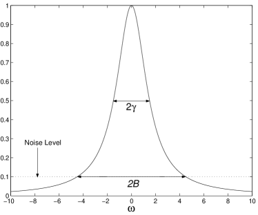
Figure 5: The dimensionless quantities $\gamma^{2}/(\gamma^{2}+\omega^{2})$ and $N$ are plotted, showing their frequency dependence (or lack of it). In this plot $\gamma=1.5$ and $N=0.1$. The frequency at which the vacuum signal drops in power to that of the noise is equal to the effective bandwidth $B$.

In terms of physical parameters

$$B=\frac{e}{2C}\sqrt{\frac{\eta{\rm P}}{k_{{\rm B}}TR\hbar\omega_{0}}}\,.$$ (92)

The photon flux ${\rm P}/\hbar\omega_{0}$ of the LO cannot be increased arbitrarily as the regime in which the photodiode responds linearly to the field incident upon it must be adhered to. The resistor $R$ cannot be reduced to zero as it is necessary for the reduction of the effective input impedance of the op-amp so that the photodiode can act as a current source. It also converts the current to a voltage, which presumably would be swamped by other, not considered, noise sources if reduced too far. Minimizing stray capacitances and the temperature of operation will improve the photoreceiver operation.

IV.3 Adding Noise Only

The limit in which the power of the Johnson noise goes to zero has already been discussed, with the result being perfect detection. If the response time of the RC circuit vanishes then, provided Johnson noise is still added, the input signal is still obscured. For this to be a physically sensible consideration we assume that the capacitance, rather than the resistance, is zero.

The output voltage of the photoreceiver is then given by

$${\cal V}=-IR+\sqrt{4k_{{\rm B}}TR}\,\frac{dW_{{\rm J}}(t)}{dt},$$ (93)

as indicated by the form of Eq. (68). Here $dW_{{\rm J}}(t)/dt$ represents the ‘real’ Johnson noise which is of a Gaussian nature. Using Eq. (69) and Eq. (85) gives (with $\Phi=0$ for convenience),

$${\cal V} \propto {\frac{\eta}{1+N}}\langle c+c^{{\dagger}}\rangle+\sqrt{\frac{\eta}{1+N}}\theta(t),$$ (94)

where $\theta(t)$ is normalized white noise consisting of a linear combination of the vacuum input noise and the Johnson noise. Comparison with Eq. (69) shows that the effect of adding noise but no filtering is to reduce the efficiency by a factor of $1+N$. It can be shown using Bayesian analysis that this result holds for the form of the quantum trajectory as well.

V Conclusion

The evolution of open quantum systems conditional upon detection results from realistic detectors cannot in general be generated by standard quantum trajectory theory (stochastic master equations). A method for generating this evolution was proposed in Ref. WarWisMab01 . The crucial element is to include correlations between the system and classical detector states which cannot be observed in practice. In this paper we have given a full description of this method, and shown how it can be applied in quantum optics. In particular, we derive realistic quantum trajectories for conditioning upon photon counting using an avalanche photodiode, and homodyne detection using a photoreceiver. These equations were presented in Ref. WarWisMab01 , but a full derivation was not given there.

In this paper we have not provided any solutions of the equations we have derived. To find and study these solutions is not a minor task, which is why it is reserved for the following paper WarWis02b . There we use our equations to determine the evolution of a two-level cavity QED system, conditioned on four different types of detection (using the two detectors mentioned above). We also consider another system which can be treated analytically for realistic homodyne detection. Our study achieves five important aims, which are outlined in the introduction to that paper.

It is worth re-emphasizing the generality of our approach. It is applicable not just in quantum optics, but in all areas where open quantum system theory is used. Prime examples are the mesoscopic measurement devices used in quantum electronics, such as single electron transistors. This device has received much attention as a possible measurement device for solid state qubits WisWah01 ; JJQubit ; Dev00 . Conditional states may be used in quantum computation both for preparation, and for non-deterministic gate implementation NieChu00 . In this context, the necessity of being able to relate realistically available results to the state of the qubit is obvious.

The greatest significance of our work is in the field of quantum control. The conditional state of a quantum system is synonymous with an observer’s knowledge about that system. Thus (assuming all uncertainties are properly taken into account) it is by definition the optimum mathematical object to use to control that system. Properly taking into account detector imperfections is essential to building optimal control loops. We thus expect our theory to have broad applications in future quantum technology.

References

- (1) J. von Neumann, Mathematical Foundations of Quantum Mechanics (Springer, Berlin, 1932); English translation (Princeton University Press, Princeton, 1955).
- (2) B. Misra and E. C. G. Sudarshan, J. Math. Phys. 18, 756.
- (3) E. B. Davies, Quantum Theory of Open Systems (Academic Press, London, 1976).
- (4) K. Kraus, States, Effects, and Operations: Fundamental Notions of Quantum Theory (Springer, Berlin, 1983).
- (5) H. J. Carmichael, An Open Systems Approach to Quantum Optics (Springer, Berlin, 1993).
- (6) J. Dalibard, Y. Castin and K. Mølmer, Phys. Rev. Lett. 68, 580 (1992).
- (7) C. W. Gardiner, A. S. Parkins, and P. Zoller, Phys. Rev. A 46, 4363 (1992).
- (8) V.P. Belavkin, “Nondemolition measurement and nonlinear filtering of quantum stochastic processes”, pp. 245-66 of A. Blaquière (ed.), Lecture Notes in Control and Information Sciences 121 (Springer, Berlin, 1988).
- (9) V.P. Belavkin and P. Staszewski, Phys. Rev. A 45, 1347 (1992).
- (10) A. Barchielli, Quantum Opt. 2, 423 (1990).
- (11) A. Barchielli, Int. J. Theor. Phys. 32, 2221 (1993).
- (12) H. M. Wiseman and G. J. Milburn, Phys. Rev. A 47, 1652 (1993).
- (13) H. M. Wiseman and G. J. Milburn, Phys. Rev. A 47, 642 (1993).
- (14) P. Warszawski, H. M. Wiseman and H. Mabuchi, Phys. Rev. A 65, 023802 (2002).
- (15) C. W. Gardiner, Quantum Noise (Springer, Berlin, 1991).
- (16) C. W. Gardiner, Handbook of Stochastic Methods (Springer, Berlin, 1985).
- (17) G. E. P. Box and G. C. Tiao, Bayesian Inference in Statistical Analysis (Addison-Wesley, Sydney, 1973).
- (18) T. P. McGarty, Stochastic Systems and State Estimation (Wiley-Interscience Publication, Sydney, 1974).
- (19) A. C. Doherty et al., Phys. Rev. A 62, 012105 (2000).
- (20) J. Gambetta and H. M. Wiseman, Phys. Rev. A 64, 042105 (2001).
- (21) J.-I. Cirac, P. Zoller, H. J. Kimble, and H. Mabuchi, Phys. Rev. Lett. 78, 3221 (1997).
- (22) A. C. Doherty and K. Jacobs, Phys. Rev. A 60, 2700 (1999).
- (23) P. Warszawski and H.M. Wiseman, following paper.
- (24) H. M. Wiseman, Phys. Rev. A 49, 2133 (1994).
- (25) H. M. Wiseman, Mod. Phys. Lett. B 9, 629 (1995).
- (26) H. M. Wiseman and L. Diósi, Chem. Phys. 268, 91 (2001); erratum 271, 227 (2001).
- (27) L. Hardy, quant-ph/0101012; L. Hardy, ”Why Quantum Theory?” in Non-locality and modality, edited by Tomasz Placek and Jeremy Butterfield (Kluwer, to be published), quant-ph/0111068.
- (28) G. Lindblad, Commun. Math. Phys. 48, 199 (1976).
- (29) B. T. Debney and A. C. Carter, Optical Fiber Sensors Components and Subsystems, Ch. 4, Vol. 1 (Artech House, Boston 1996).
- (30) B. Garside, Optical Fiber Sensors Components and Subsystems, Ch. 5, Vol. 3 (Artech House, Boston 1996).
- (31) J. D. C. Jones, Optical Fiber Sensor Technology, Ch. 4 (Chapman and Hill, London 1995).
- (32) S. Takeuchi, J. Kim, Y. Yamamoto and H. H. Hogue, Appl. Phys. Lett. 74, 1063 (1999).
- (33) A. Lacia et al., Appl. Phys. Lett. 62, 606 (1993).
- (34) H. Mabuchi, California Institute of Technology, private communication.
- (35) H. M. Wiseman et al., Phys. Rev. B 63, 235308 (2001).
- (36) M. H. Devoret and R. J. Schoelkopf, Nature 406, 1039 (2000).
- (37) G. Schön, A. Shnirman and Y. Makhlin, cond-mat/9811029.
- (38) M. A. Nielsen and I. L. Chuang, Quantum Computation and Quantum Information (Cambridge University Press, 2000).