Adaptive quantum-limited estimates of phase

Abstract

Quantum-limited estimation of an optical phase using adaptive (i.e. real-time feedback) techniques is reviewed. One case is explored in detail, as it can be understood using only elementary concepts such as photonic shot-noise and error analysis. Very recent experimental results are discussed.

I Introduction

Having been working on the topic of quantum-limit adaptive estimation of optical phase for some years now Wis95 ; WisKil97 ; WisKil98 ; BerWisZha99 ; BerWis00 ; BerWis01a ; BerWis01b ; BerWisBre01 ; BerWis02 , when I (HMW) was asked to contribute an article on it, the question “why now?” naturally arose. I believe there are three good answers to this question. In order of increasing importance,

1. The work done by me, and more particularly my students, covers a wide range of cases. It is only now that it is possible to put them all in an overall context.

2. Some of the latest results are actually the easiest to explain to a non-specialist.

3. The first experiments verifying the theory have very recently been performed in the laboratory of Hideo Mabuchi at CalTech.

Before discussing these interesting developments, I should explain what quantum-limited adaptive phase estimation means. The phase in question is an unknown (and possibly varying) optical phase ${\varphi}$. The aim is to estimate this phase, on the basis of measurements, as well as quantum mechanics allows. The allowed resources are practical ones: photodetectors, electronics, and linear (electro-)optics. The fundamental limitation is the number of photons (per pulse or per coherence time). There are also many practical limitations such as efficiency, the source of light, time delays, and processing limitations. These have all been considered WisKil97 ; BerWisZha99 ; BerWis01a ; BerWis01b , but for simplicity I will not discuss them here.

Where adaptive estimation comes in is that to realise the above aim using the allowed resources it turns out that it is necessary to use real-time feedback during the measurement. The basic idea is as follows. If ${\varphi}$ is known to a very good approximation, then a simple measurement scheme will usually give near-optimal results. An example is homodyne measurement of the phase quadrature of a pulse WalMil94 . However if ${\varphi}$ is totally unknown then the standard solution is to measure both quadratures (e.g. by heterodyne detection). This is far from optimal. The alternative is adaptive detection: use the results so far in the measurement to make an estimate ${\hat{\varphi}}$ of ${\varphi}$, and use this in a feedback loop to make the rest of the measurement closer to optimal.

I believe this work is important for a number of reasons:

First, quantum phase has a long and controversial history PegBar97 . Although ideal phase measurements can be defined, there is no way to make them without optical materials with arbitrarily high orders of nonlinearity WisKil98 . Hence it is of fundamental interest to know how well one can do with linear devices.

Second, with continued miniaturisation of devices there will come a time when quantum limits do set the fundamental limits for technology. There is every reason to expect that phase estimation, as required for phase locking loops for example, will still be a practical concern then.

Third, the idea of adaptive measurements may have applications far beyond that of phase measurements, so the theoretical and experimental expertise gained here potentially opens new frontiers in quantum measurement theory. It also has implications for the way in which we understand phenomena such as the “collapse of the wavefunction”.

Finally, the cutting-edge technology required for quantum-limited adaptive measurements is a stepping stone towards more general methods for controlling quantum systems, another area of future importance as engineering heads towards the quantum realm. As will be discussed in Sec. V, the new technology being applied is both electronic and optical.

II Overview of Past Results

There are many different cases that can be considered, and they can be systematised by considering the following four questions:

1. Is the detection dyne (that is, using an optical local oscillator) or interferometric?

2. Is the light source coherent (e.g. a laser), or nonclassical (e.g. squeezed)?

3. Is the scheme non-adaptive, or adaptive?

4. Is it single-shot with a single phase, or CW with a varying phase?

Two of these distinctions definitely require further explanation.

First, dyne versus interferometric detection. These are illustrated in the figures below.

Figure 1: Adaptive phase estimation: dyne detection (top) and interferometric detection (bottom). BS = Beam Splitter, and dashed lines are optical paths.

It might well be objected that dyne detection (of which homodyne and heterodyne are two examples WisKil97 ) is merely one sort of interferometric measurement HarSan96 , in that the local oscillator is interfered with the signal light before detection. This is quite true; I am using the two terms to make a distinction between how the accounting is done. In dyne detection only the signal pulse or beam is treated as quantum, and only the number of photons in it is counted for the purposes of determining the quantum limit. In interferometric detection both input pulses or beams into the Mach-Zehnder interferometer are treated as quantum, and the photon number in both is counted BerWis00 ; BerWisBre01 . There is also a practical distinction in that dyne detection uses a photoreceiver that yields a photocurrent which does not distinguish individual photons, whereas interferometric detection uses photon counters. In both cases the aim is to measure the phase $\varphi$; in the former this phase is defined relative to the local oscillator, while for the latter it is as a relative phase between the two arms of the interferometer.

Second, single-shot versus CW. In a single-shot measurement, there is a single pulse of light (which may however be split over two modes for the case of interferometric detection). There is a single unknown phase $\varphi$ imprinted on the pulse. The relevant parameter for the fundamental limit is $n$ (or $\bar{n}$), the (mean) number of photons in the pulse. In Continuous-Wave detection, there is a beam (or two beams in the interferometric case) of light. A time-varying phase $\varphi(t)$ is imprinted on (one of) the beam(s). In this article I will consider only the case where the time variation is that of white noise. That is,

$$\dot{\varphi}=\sqrt{\kappa}\,{\xi}(t).$$ (1)

This could arise from thermal mechanical fluctuations of miniaturised optical elements, for example. The parameter $\kappa$ is the rate of phase diffusion, or, equivalently, the resulting linewidth of the beam. The relevant parameter in this case is $N$, the mean number of photons per coherence time: $N=P/\hbar\omega{\kappa}$, where $P$ is the beam power.

Having explained the various cases, I can now give the promised overview. The simplest results arise by considering the mean square error (MSE) in the estimated phase, in the asymptotic limit where $n$ or $\bar{n}$ or $N$ go to $\infty$. The results for the MSE scale as in table 1.

		dyne		interferometric
		coherent	non-class.	coherent	non-class.
	adaptive	$0.5/N^{1/2}$	$\underline{\sim 1/N^{2/3}}$	$1/N^{1/2}$	${?}\phantom{\stackrel{{\scriptstyle?}}{{\sim}}}$
CW	non-adapt.	$0.71/N^{1/2}$	${0.66/N^{1/2}}$	$1/N^{1/2}$	${?}\phantom{\stackrel{{\scriptstyle?}}{{\sim}}}$
single	adaptive	$0.25/\bar{n}$	$\underline{\sim\log\bar{n}/\bar{n}^{2}}$	$1/n$	$\underline{\stackrel{{\scriptstyle?}}{{\sim}}\log n/n^{2}}$
shot	non-adapt.	$0.5/\bar{n}$	${0.25/\bar{n}}$	$1/n$	${\sim 1/n}\phantom{\stackrel{{\scriptstyle?}}{{\sim}}}$

Table 1: Asymptotic mean square errors for phase estimation. The results that beat the standard quantum limits are underlined.

There is a good deal of regularity in this table, as the reader may discern. I wish to draw attention to one feature in particular. The sixteen MSEs (some still undetermined) can be divided into four squares of four MSEs. In each square for which results are fully known, three of the MSEs scale in the same way. This scaling represents the standard quantum limit (SQL) for that particular case. The fourth, underlined in the above table, beats the SQL. In each case, this requires both non-classical light and adaptive detection.

III Latest Results: CW Dyne Detection

To try to explain adaptive phase estimation in more detail, I will concentrate now on the particular case of CW dyne detection. This is one the latest areas to be investigated, by Dominic Berry and myself BerWis02 , but turns out to be probably the simplest to explain. To reiterate the basic idea, we want the best estimate of the current value of $\varphi(t)$ which obeys $\dot{\varphi}=\sqrt{\kappa}\,{\xi}(t),$ where $\xi(t)$ is white noise with unit spectral power.

Consider first the case of coherent light of power ${P}=\hbar\omega{\alpha}^{2}$, detected by interfering with a local oscillator at a balanced photoreceiver. The resulting dyne photocurrent, suitably scaled, is WisKil97

$${I}(t)=2{\alpha}\cos[\Phi(t)-{\varphi}(t)]+{\zeta}(t),$$ (2)

where $\Phi(t)$ is the local oscillator phase, and $\zeta(t)$ is another Gaussian white noise term, independent of $\xi(t)$, with unit spectral power. It can be thought of as local oscillator shot noise, or vacuum noise. In any case, it is quantum noise.

The standard non-adaptive technique to estimate phase is to vary $\Phi(t)$ over all phases. This can be achieved by heterodyne detection with a detuning $\Delta\gg\sqrt{\alpha\kappa}$, which makes $\Phi$ vary as $\Phi(t)=\Phi(0)+\Delta\times t$. From Eq. (2), we would expect better sensitivity if we were to choose $\Phi(t)$ to maximise the slope of $\cos[\Phi(t)-{\varphi}(t)]$. That is, we should set ${\Phi}(t)={\hat{\varphi}}(t)+\pi/2$ so that

$${I}(t) = 2{\alpha}\sin[{\varphi}(t)-{\hat{\varphi}}(t)]+{\zeta}(t)$$ (3)

$$\simeq 2{\alpha}[{\varphi}(t)-{\hat{\varphi}}(t)]+{\zeta}(t),$$

for ${\hat{\varphi}}(t)\simeq{\varphi}(t)$. The question is, how should we choose the estimate ${\hat{\varphi}}(t)$?

One obvious possibility is to choose it from the immediately preceding photocurrent. We can rearrange Eq. (3) to get

$${\varphi}(t)\simeq\left[{{\hat{\varphi}}(t)+\frac{{I}(t)}{2{\alpha}}}\right]+\frac{{\zeta}(t)}{2{\alpha}}.$$ (4)

For a given ${\hat{\varphi}}(t)$, we could thus form

$${\hat{\varphi}_{\rm imm}}(t+\delta t)=\frac{1}{\delta t}\int_{t}^{t+\delta t}\left[{{\hat{\varphi}}(t)+\frac{{I}(s)}{2{\alpha}}}\right]ds.$$ (5)

This has the MSE

$${\sigma^{2}_{\rm imm}}(t+\delta t) = \left\langle{[{\hat{\varphi}_{\rm imm}}(t+\delta t)-{\varphi}(t+\delta t)]^{2}}\right\rangle$$ (6)

$$\simeq \frac{1}{4{\alpha}^{2}\delta t}.$$

This diverges as $\delta t\to dt$, so clearly ${\hat{\varphi}_{\rm imm}}$ is not a good estimate. Instead, we need a ${\hat{\varphi}}(t)$ that involves a finite time average.

The optimal time-average for ${\hat{\varphi}(t)}$ can be determined as follows. Say the MSE in ${\hat{\varphi}}(t)$ is ${\sigma^{2}}(t)$. Over the interval $[t,t+\delta t)$, the diffusion of ${\varphi}(t)$ causes this to increase to

$${\sigma^{2}_{\rm old}}(t+\delta t) = \left\langle{[{\hat{\varphi}}(t)-{\varphi}(t+\delta t)]^{2}}\right\rangle$$ (7)

$$= \left\langle{[{\hat{\varphi}}(t)-{\varphi}(t)]^{2}}\right\rangle+\left\langle{[{\varphi}(t)-{\varphi}(t+\delta t)]^{2}}\right\rangle$$

$$= {\sigma^{2}}(t)+{\kappa}\delta t.$$

By standard error analysis, the optimal ${\hat{\varphi}}(t+\delta t)$ weights ${\hat{\varphi}}(t)$ and ${\hat{\varphi}_{\rm imm}}(t+\delta t)$ appropriately:

$${\hat{\varphi}}(t+\delta t)={\sigma^{2}}(t+\delta t)\left[{\frac{{\hat{\varphi}_{\rm imm}}(t+\delta t)}{{\sigma^{2}_{\rm imm}}(t+\delta t)}+\frac{{\hat{\varphi}}(t)}{{\sigma^{2}_{\rm old}}(t+\delta t)}}\right],$$ (8)

where

$$\frac{1}{{\sigma^{2}}(t+\delta t)}=\frac{1}{{\sigma^{2}_{\rm imm}}(t+\delta t)}+\frac{1}{{\sigma^{2}_{\rm old}}(t+\delta t)}.$$ (9)

Taking $\delta t\to dt$ yields a differential equation for $\sigma^{2}(t)$ that has the stationary solution

$$\sigma^{2}=1/2\sqrt{{N}}~{},~{}~{}{\rm where}~{}{N}={\alpha}^{2}/{\kappa}.$$ (10)

Substituting this into Eq. (8) gives $d{\hat{\varphi}}(t)=(\kappa/\sigma^{2})\times({I}(t)dt/2{\alpha}).$ Since the feedback sets $\Phi(t)=\hat{\varphi}(t)+\pi/2$, the feedback algorithm is simply

$$\dot{\Phi}=\frac{\kappa}{\sigma^{2}}\frac{{I}(t)}{2{\alpha}}.$$ (11)

By way of comparison, for heterodyne (nonadaptive) detection, the stationary MSE can be shown to be BerWis02

$$\sigma^{2}_{\rm het}=1/\sqrt{2{N}}.$$ (12)

That is, the adaptive technique offers a factor of $1/\sqrt{2}$ improvement in the mean square error.

IV What is quantum about it?

This is a question I am often asked. A feedback algorithm of the form

$$\dot{\Phi}={\chi}{I}(t)/2{\alpha}$$ (13)

looks like a standard low frequency classical phase-locking algorithm with gain $\chi$. The quantum feature is that the optimal value of ${\chi}$ is finite:

$${\chi_{\rm opt}}=\frac{\kappa}{\sigma^{2}}=2\sqrt{\kappa}{\alpha}.$$ (14)

In the classical limit (with no other noise sources), $\chi_{\rm opt}$ would be infinite, as can be seen by writing it explicitly in terms of classical quantities and $\hbar$:

$$\chi_{\rm opt}=2\sqrt{{\kappa}{P}/\hbar\omega}.$$ (15)

For general ${\chi}$, the stationary MSE can be shown to be

$$\sigma^{2}=\frac{\chi}{8{\alpha}^{2}}+\frac{\kappa}{2{\chi}},$$ (16)

which diverges as ${\chi}\to\infty$. Moreover, if $\chi$ differed from $\chi_{\rm opt}$ by a factor greater than about $2.4$ (in either direction), then all advantage gained by doing an adaptive detection would be lost. That is, the MSE would become greater than that which can be achieved by the nonadaptive technique of heterodyne detection (12).

The advantage offered by adaptive detection is only a constant factor (of $1/\sqrt{2}$) because so far I have discussed only coherent light. To break the SQL scaling $\sigma^{2}\sim{N}^{-1/2}$ it is necessary to use nonclassical light. The most obvious sort of nonclassical light to consider for this situation is broad-band squeezed light Bac98 . This is light where the spectrum of the dyne photocurrent of one quadrature, normalised as in Eq. (2), has a noise spectrum $S$ below unity over some bandwidth broad compared to $\sqrt{\kappa\alpha}$. For moderate phase quadrature squeezing of spectral noise ${S}$, we can use the same feedback algorithm (13) to get an improvement in the MSE by a factor of $\sqrt{S}$:

$$\sigma^{2}=\sqrt{S}/2\sqrt{N}~{},~{}~{}{\rm for}~{}{\chi}={\kappa}/\sigma^{2}.$$ (17)

It would appear from this that the MSE in the phase estimate could be made as small as one desires by making the phase quadrature more squeezed. However this is not the case because the noise gets “squeezed” into the amplitude quadrature of the light Bac98 ; WalMil94 . Because the local oscillator phase $\Phi$ is only orthogonal to the estimated system phase $\hat{\varphi}$, not the true phase $\varphi$, the amplitude fluctuations do contribute to the noise in the phase measurement. It can be shown that as a consequence there is an optimal non-zero squeezing spectrum ${S}\sim{N}^{-1/3}$. This is, in a sense, a “more quantum” feature than the existence of shot noise which gave the above limit (10), because it is a consequence of the uncertainty relation between amplitude and phase for a light beam WalMil94 . In any case, with squeezed light we can beat the SQL, and find a new quantum limit for CW phase locking:

$$\sigma^{2}\sim{N}^{-2/3}.$$ (18)

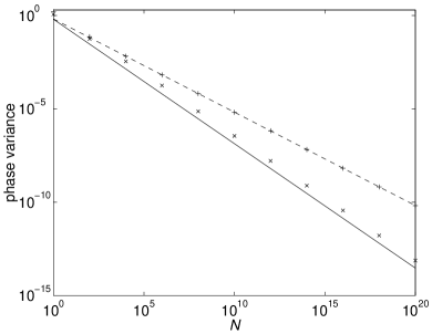
Figure 2: Numerical results for the mean square phase error using optimal squeezing, for heterodyne (+) and adaptive (x) detection. Note that these were obtained using a more sophisticated feedback algorithm than that explained above. The analytical asymptotic results are: heterodyne (– –), $0.66/N^{1/2}$ and adaptive (—), $0.63/N^{2/3}$.

V Experimental Progress

Performing a quantum-limited adaptive phase measurement has been one of the primary research objectives of Assoc. Prof. Hideo Mabuchi since his appointment at CalTech in 1999. As mentioned in the introduction, this is the first step towards a longer-term goal of investigating quantum-limited control in general, and in particular in cavity QED systems. This first step has proven quite challenging in its own right!

Rather than a CW measurement of a varying phase as discussed above, Mabuchi’s group has been working on single-shot estimates of an unknown phase imprinted on a pulse of light, as originally considered in Ref. Wis95 . Here the parameter $\bar{n}$ (see table 1) is simply the mean number of photons in a single pulse on which a single unknown phase is imprinted. For an adaptive measurement, the phase must be estimated when only a fraction of these $\bar{n}$ photons have entered the detector. The fact that this can work even for $\bar{n}$ of order unity is described by Mabuchi as a “pretty wild fact that makes you think twice about field quantisation”.

In this single-shot case the feedback algorithm is considerably more complicated than that in Sec. IV, as the local oscillator phase $\Phi(t)$ may depend nonlinearly upon various integrals of the photocurrent during the course of a single pulse BerWis01a . The form of these integrals can only be derived from the full quantum theory WisKil98 . Mabuchi thus decided to use digital electronics, and to discretise the feedback algorithm.

Just as the CW result requires the magnitude of the feedback $\chi$ to be close to its theoretical optimum (as discussed in Sec. IV), the single shot case is sensitive to the design of the feedback loop. Through numerical modeling, Mabuchi’s group have found that the discretisation requires at least of order 100 divisions of the total pulse length $T$.

The only electronics fast enough to do the required processing are field programmable gate arrays Sto02 . These are so fast (10s of MHz) that the feedback bandwidth, of around 5 MHz, is actually limited by the the bandwidth of the electro-optics (in particular the synthesiser used to modulate the feedback). This bandwidth allows each time-division to be of order $500$ns, for a total time $T$ of only about $50\mu$s. This still required the production of a coherent state of this duration. In other words, it required light with a shot-noise limited amplitude spectrum down to about 50 kHz. This was another enormous technical challenge, as this is far below the usual frequency regime of quantum-limited experiments Bac98 . It was achieved using a very high Q cavity of lifetime 16 $\mu$s as a mode cleaner.

Because they are not (as yet) using any non-classical source, the experimental signature Mabuchi’s group is seeking is a reduction of the MSE (by at most a factor of 2 — see table 1) below the heterodyne limit of $0.5/\bar{n}$. In work just released to the physics archive Arm02 , this reduction has been convincingly demonstrated. Of course, much work remains to be done. For example, Mabuchi plans to investigate the tails of the distribution as well as its standard error, to verify some of the predictions of Ref. WisKil98 . Employing non-classical light to break the SQL is another longer term goal. Other experimental groups are interested in this as well.

VI Conclusions

Estimating an unknown phase ${\varphi}$ at the quantum limit is a difficult problem. There are many different cases that can be considered, but for all of them the standard quantum limits (SQLs) for the mean-square error arise for coherent light or non-adaptive measurements. The SQLs can be beaten only by using nonclassical light in conjunction with adaptive measurements. When devices including phase-locking loops are sufficiently miniaturised, quantum limits will become practical limits. Thus, as well as being of theoretical interest, adaptive measurements should become part of the tool-kit of the future “quantum engineer” who seeks to manipulate quantum systems as well as nature allows.

The improvement offered by adaptive detection over non-adaptive detection in phase estimation has very recently been achieved by the group of Hideo Mabuchi at CalTech. This experiment breaks new ground in the use of low-frequency optical mode cleaning and high-speed digital electronics in quantum-limited experiments. The theoretical and experimental techniques developed also pave the way for future research into the feedback-control of quantum optical systems in general.

References

- (1) H.M. Wiseman, Phys. Rev. Lett. 75, 4587 (1995).
- (2) H.M. Wiseman and R.B. Killip, Phys. Rev. A 56, 944 (1997).
- (3) H.M. Wiseman and R.B. Killip, Phys. Rev. A 57, 2169 (1998).
- (4) D. Berry, H.M. Wiseman, and Zhong-Xi Zhang, Phys. Rev. A 60, 2458 (1999).
- (5) D.W. Berry and H.M. Wiseman, Phys. Rev. Lett. 85, 5098 (2000).
- (6) D. Berry and H.M. Wiseman, Phys. Rev. A 63, 013813 (2001).
- (7) D.W. Berry and H.M. Wiseman, J. Mod. Optics. 48, 797 (2001).
- (8) D. W. Berry, H. M. Wiseman and J. K. Breslin, Phys. Rev. A. 63, 053804 (2001).
- (9) D.W. Berry and H. M. Wiseman, Phys. Rev. A. 65, 043803 (2002).
- (10) D. F. Walls and G. J. Milburn, Quantum Optics (Springer, Berlin, 1994).
- (11) D. T. Pegg and S. M. Barnett, J. Mod. Opt. 44, 225 (1997).
- (12) P. Hariharan and B. C. Sanders, Progress in Optics XXXVI, 49 (1996).
- (13) J. Stockton, M. Armen, and H. Mabuchi, “Programmable Logic Devices in Experimental Quantum Optics”, quant-ph/0203143
- (14) H-A. Bachor, A Guide to Experiments in Quantum Optics (Wiley, 1998)
- (15) M. A. Armen, J. K. Au, J. K. Stockton, A. C. Doherty, and H. Mabuchi, “Adaptive homodyne measurement of optical phase”, quant-ph/0204005