Quantum Trajectories for Realistic Photodetection II: Application and Analysis

Abstract

In the preceding paper [Warszawski and Wiseman] we presented a general formalism for determining the state of a quantum system conditional on the output of a realistic detector, including effects such as a finite bandwidth and electronic noise. We applied this theory to two sorts of photodetectors: avalanche photodiodes and photoreceivers. In this paper we present simulations of these realistic quantum trajectories for a cavity QED scenario in order to ascertain how the conditioned state varies from that obtained with perfect detection. Large differences are found, and this is manifest in the average of the conditional purity. Simulation also allows us to comprehensively investigate how the quality of the the photoreceiver depends upon its physical parameters. In particular, we present evidence that in the limit of small electronic noise, the photoreceiver quality can be characterized by an effective bandwidth, which depends upon the level of electronic noise and the filter bandwidth. We establish this result as an appropriate limit for a simpler, analytically solvable, system. We expect this to be a general result in other applications of our theory.

I Introduction

In the preceding paper WarWis02a we gave a full description of a method to model the evolution of open quantum systems conditional upon detection results from realistic detectors. This is a generalization of standard quantum trajectory theory, to take into account correlations between the system and classical detector states which cannot be observed in practice. We also showed how it can be applied in quantum optics, deriving realistic quantum trajectories for conditioning upon photon counting using an avalanche photodiode (APD), and homodyne detection using a photoreceiver (PR). The greatest significance of our work is in the field of quantum control, where conditional states are the optimal basis for control loops.

In this paper we find and study solutions to the realistic quantum trajectory equations derived in the preceding paper. We consider the evolution of a two-level cavity QED system (which for convenience we refer to as a two-level atom), conditioned on four different types of detection (using the two detectors mentioned above). Some of these solutions have been studied in a previous paper by us and Mabuchi WarWisMab01 , but not with the thoroughness we apply here. These solutions can only be found numerically, because of the nonlinearity of the system. We also consider another system, the degenerate parametric oscillator below threshold (DPOBT), which can be treated analytically for realistic homodyne detection.

Our study in this paper achieves five important aims. First, it shows how the theory developed in the preceding paper is implementable in practice. Second, it establishes the degree of impact of detection imperfections on the purity of the conditional system state. Third, it illustrates how realistic quantum trajectories typically differ from standard (idealized) quantum trajectories, which helps to build intuition about them. Fourth, it emphasizes the importance of the experimenter’s choice of detection scheme in determining how well one can follow the conditional evolution of a system. Fifth, it allows us to quantitatively investigate emergent properties of realistic trajectories, such as the “effective bandwidth” discussed in the preceding paper.

This paper is organized as follows. We begin in Sec. II by introducing the two-level atom (TLA) that will be the subject of study for most of the remainder of the paper. We also consider standard (idealized) quantum trajectories for this system under the four different measurement schemes we consider. In Sec. III we discuss the idea of levels of conditioning. These arise from different levels of knowledge a hypothetical observer has about the dynamics of the detector. They help one to understand how realistic trajectories differ from idealized trajectories. In Sec. IV we analyze the stochastic dynamics of the system under two realistic detection schemes (direct and adaptive) using the APD. In Sec. V we do likewise for the two homodyne detection schemes using the PR. In Sec. VI we return to the question of effective bandwidth for the PR, discussed in Sec. IV B of the preceding paper. We verify the formula suggested in the preceding paper, numerically for the TLA and analytically for the DPOBT. Sec. VII contains a discussion of the numerical techniques used in our simulations, and Sec. VIII concludes.

II The Two-Level System

II.1 The system

A driven ($\Omega$) and damped ($\gamma$) two-level atom (TLA) is the smallest (in Hilbert space) quantum optical system. However, it is a nonlinear system and has surprisingly rich dynamics. These are especially evident when one considers conditioning on measurements of its fluorescence DalCasMol92 ; wtime ; WisMil93c ; WisToo99 . For this reason, we use it as a test system for investigating realistic photodetection.

In reality it would be almost impossible to collect and detect all, or even most, of the fluorescence of an atom in free space. It is therefore better to envisage our two-level quantum system as a cavity-QED system consisting of a single two-level atom strongly coupled ($g$) to an optical cavity which is even more strongly damped ($\kappa$). In the limit $\kappa\gg g,\Omega\gg\gamma$, the light emitted by the atom into the cavity damps through the cavity end-mirror to form an output with the same temporal properties as the free-space fluorescence. If $g^{2}/\kappa\gg\gamma$, the free-space damping may be ignored and the effective damping rate of the two-level system is $\Gamma=g^{2}/\kappa$. We have this in mind when choosing parameters for our simulations. The advantage of this scheme is of course that the cavity output beam is readily measurable, by photon counting or homodyne detection.

Let us denote the ground and excited states for the TLA by $|{g}\rangle$ and $|{e}\rangle$. Defining the Pauli matrices in the usual manner, the state matrix for the TLA can be written as

$$\rho=\mbox{$\frac{1}{2}$}\left(I+x\sigma_{x}+y\sigma_{y}+z\sigma_{z}\right),$$ (1)

where $(x,y,z)$ is the Bloch vector which is confined to a unit-sphere. The purity of the TLA can be defined as

$${\rm purity}={\rm Tr}[\rho^{2}]=\mbox{$\frac{1}{2}$}\left(1+x^{2}+y^{2}+z^{2}\right).$$ (2)

It has an upper limit of $1$ (a pure state) and lower limit of $\frac{1}{2}$ (a completely mixed state).

The unconditioned ME for the driven and damped TLA in the interaction picture is

$$\dot{\rho}=-i\frac{\Omega}{2}\left[\sigma_{x},\rho\right]+{\cal D}[c]\rho\equiv{\cal L}\rho.$$ (3)

Here $c=\sqrt{\Gamma}\sigma$, where $\sigma$ is the TLA lowering operator. The steady state solution of this ME is

$$\rho=\frac{\Omega^{2}+\Omega\Gamma\sigma_{y}+\Gamma^{2}\left(1-\sigma_{z}\right)/2}{2\Omega^{2}+\Gamma^{2}},$$ (4)

which has a purity of

$$p_{{\rm ME}}=1-2\left(\frac{\Omega^{2}}{2\Omega^{2}+\Gamma^{2}}\right)^{2},$$ (5)

which goes to $1$ for small $\Omega$ and to $\frac{1}{2}$ for large $\Omega$.

II.2 Perfect Direct Detection

Let us now consider continuous, perfect measurement of the TLA. Firstly consider counting photons in the emitted field. In the preceding paper we stated the relevant stochastic master equation (SME) in Sec. II C. With efficiency $\eta=1$ it is

$$d\rho = -\,dt{\cal H}[iH+\mbox{$\frac{1}{2}$}c^{{\dagger}}c+\mu^{*}c+\mbox{$\frac{1}{2}$}|\mu|^{2}]\rho$$ (6)

$${+}\,dN(t){\cal G}[(c+\mu)]\rho.$$

Here ${\rm E}[dN(t)]={\rm Tr}[(c^{{\dagger}}+\mu^{*})(c+\mu)\rho]dt$, and $\mu$ is the (necessarily small) local oscillator (LO) amplitude. See the preceding paper for definitions of the superoperator symbols ${\cal H}$ and ${\cal G}$. A typical quantum trajectory for direct detection (for which $\mu=0$) is shown in Fig. 1, where plots of $x,y,z$ specify the system state.

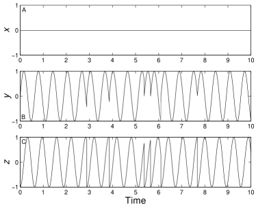
Figure 1: A typical trajectory for direct detection for $\Omega=10\Gamma$. The two quadratures of the TLA are shown ($x$ in plot (A) and $y$ in plot (B)) as is the inversion, $z$, of the TLA (in plot (C). Time is measured in units of $\Gamma^{-1}$. This is true for the remainder of this paper, unless otherwise stated.

The $x$ quadrature is zero since the Hamiltonian is proportional to this quadrature. For this reason we can envisage the TLA moving in the $y$–$z$ plane of the Bloch sphere. Since $\Omega\gg\Gamma$ for this trajectory, the $y$ value of the state oscillates between $-1$ and $1$ between jumps. The coherent driving also causes the inversion of the TLA, $z$, to oscillate between $-1$ (ground state) and $1$ (excited state). Jumps (photon detections) take $z$ to $-1$ and $y$ to $0$ as expected. The conditional purity is of course unity at all times. The average photon flux entering the detector can be calculated from Eq. (4) to be

$$f_{{\rm direct}}=\frac{\Gamma\Omega^{2}}{2\Omega^{2}+\Gamma^{2}}.$$ (7)

This saturates at $\Gamma/2$ for $\Omega\gg\Gamma$, as is consistent with the number of jumps seen in Fig. 1.

II.3 Perfect Adaptive Detection

A quite different sort of conditional dynamics are revealed using the adaptive detection scheme proposed in WisToo99 . In this scheme the output field from the TLA is combined with a weak LO at a low reflectivity beam splitter, before being subjected to direct detection (see Fig. 2). The local oscillator amplitude $\mu$ in Eq. (6) is chosen to be $\pm\sqrt{\Gamma}/2$. Two values are present here because the LO amplitude is flipped following each detection. This is what makes the scheme adaptive: the measurement being made at any particular time depends on the past results.

Figure 2: Adaptive detection, with the low intensity LO amplitude controlled by the output of the photodetector. See text for further details.

With this $\mu=\pm\sqrt{\Gamma}/2$ and the $\Omega\sigma_{x}/2$ Hamiltonian, the behaviour of the TLA is very simple. After transients have passed, the state just jumps between two fixed states that are close to $x$ eigenstates (for $\Omega\gg\Gamma$). These two states are actually the stable eigenstates of the two ($\pm$) no-detection measurement operators (see, for example, Ref. Wis96a ) When a detection on the combined field occurs, the TLA jumps into the stable eigenstate of the other no jump operator. A typical trajectory for adaptive detection is shown in Fig. 3 for $\Omega=10\Gamma$. The two-state jumping is clearly evident. Note that $y$ and $z$ take on the same values in both of the two stable states.

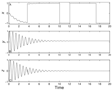
Figure 3: A typical trajectory for adaptive detection with $\Omega=10\Gamma$. Two state jumping is clearly visible.

The actual photon flux entering the photodetector for perfect adaptive detection can be calculated using the eigenstates of the no-jump operator, which are given in Ref. WisToo99 . In either eigenstate it is

$$f_{{\rm adapt.}}=\frac{\Gamma}{4}.$$ (8)

Again, this is consistent with the number of jumps in Fig. 3 (note the longer time interval displayed).

II.4 Perfect Homodyne Detection

In homodyne detection the LO is so strong that individual photons cannot be resolved, and the measurement result is a current with white noise $\xi(t)$. For perfect homodyne detection the quantum trajectory for the system is generated by the SME

$$d\rho_{I}=dt\left\{{\cal L}+\xi(t){\cal H}[e^{-i\Phi}c]\right\}\rho,$$ (9)

which results from the SME in Sec. II C 2 of the preceding paper with $\eta=1$. Here $\Phi$ is the phase of the LO.

Homodyne $x$ detection ($\Phi=0$) corresponds to an ‘unsharp’ measurement of the $x$ quadrature. With a $\sigma_{x}$ Hamiltonian, only the measurement causes $x$ to become non-zero. Thus, $x$ tends to be projected into an $x$ eigenstate, with motion between the two eigenstates on the time scale of $\Gamma$. This behaviour was first noted in Ref. WisMil93c . A typical trajectory for $\Omega=10\Gamma$ is shown in Fig. 4. The $\Omega$ oscillations of $y$ and $z$ are non-maximal, and are noisy due to the white noise in Eq. (9).

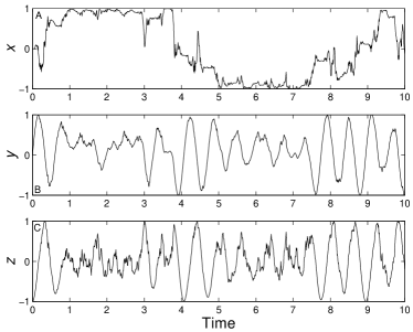
Figure 4: A typical trajectory for homodyne $x$ detection with $\Omega=10\Gamma$.

In homodyne $y$ detection ($\Phi=-\pi/2$), the $y$ quadrature is measured, which pushes the TLA state closer to the $y$ eigenstates. Unlike for the $x$ measurement though, the $\Omega$ dynamics quickly rotate $y$ away from the eigenstate. as seen in Fig. 5. As there is no measurement or driving of the $x$ quadrature, it remains strictly zero, so the oscillations of $y$ and $z$ are maximal.

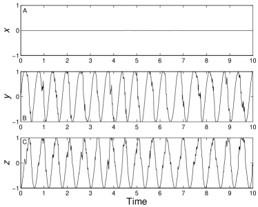
Figure 5: A typical trajectory for homodyne $y$ detection with $\Omega=10\Gamma$.

III Levels of Conditioning

To explicitly show how realistic detection conditions the state of the TLA differently from perfect detection, it is useful to re-introduce the hypothetical observer of the preceding paper (here known as the ‘perfect’ observer). This observer is able to perfectly monitor the system output as it is absorbed by the realistic detector. A further observer is introduced who is able to access only the microscopic states of the detector. In the case of the APD this corresponds to knowledge of whether the state is $0$, $1$ or $2$. For the PR, this ‘intermediate’ observer knows the voltage across the capacitor. Hence this observer avoids some, but not all, of the detector imperfections. Since the detector is being treated classically, the perfect and intermediate observers do not affect the average detector state because there are no detector superpositions to collapse. Hence they are consistent with the final ‘realistic’ observer who has access only to the realistic experimental records. In the notation of the preceding paper, these records are $d{\cal N}(t)$ and ${\cal V}(t)$ for the APD and PR, respectively.

Although the measurement records of the three observers are obviously different, they can be generated from the same experimental run. The observers are monitoring the TLA at the same time, but have varying levels of access to the pool of data that could optimally be gained from the behaviour of detector. This means that correlations between the records exist that will be revealed in the evolution of the TLA that they prescribe. Through this analysis an understanding of how the specific features of the trajectories relate to each detector imperfection can be obtained.

At a particular time each of the three observers will attach, in general, a different state matrix, $\rho$, to the TLA. If $\rho$ represents the state of the TLA in an ontological sense then there is clearly a paradox — how could the atom have more than one state at the one time? The existence of the three observers is, in the context of the described experiment, not practical, but it is not difficult to think of a realisable experiment in which one observer must determine $\rho$ from a ‘filtered’ set of measurement results, while another has access to the complete set of results. Another trivial example is where different observers have different knowledge of the initial state of the system. However, in this latter case the observers, if they had access to the same measurement results, would eventually agree on the system state. That is, for a sufficiently long measurement record, the state is dependent upon the record only and not the initial condition. This has been shown by Doherty and co-workers Dohe99 and also applies for inefficient detection.

In Ref. Dohe99 , the authors take the view that the state is the observer’s best description of the system, taking into account initial knowledge and the measurement record. That is, $\rho$ represents the state of the system in an epistemological sense. This resolves the paradox raised in the previous paragraph, but does not rule out the possibility that there also exists a state of the system in an ontological sense. In particular, the state that the perfect observer assigns to the system is unique because it is a pure state, and no other pure state can be consistently assigned to the system BruFinMer02 . A state vector is the best possible description of the system CavesProb , and for this reason it seems that no harm can be done in saying that it represents the ‘real’ state of the quantum system. The states assigned by the intermediate and realistic observers can only be interpreted as states of knowledge.

Before leaving this discussion, it is worth saying a few words about consistency. It was already noted above that although the state matrices assigned by the three observers are different, they must be consistent. That is, the intermediate observer’s state must contain the perfect observer’s state, and the realistic observer’s state must contain the intermediate observer’s state. When we say the state of observer B ($\rho_{\rm B}$) contains the state of observer A ($\rho_{\rm A}$), we can write this as

$$\rho_{\rm A}\subseteq\rho_{\rm B},$$ (10)

which means

$$\exists\epsilon>0\;:\;\;\rho_{\rm B}-\epsilon\rho_{\rm A}\geq 0,$$ (11)

and could be read as “A knows all that B knows”. For example, if the perfect observer knows that the TLA is in the ground state, then the realistic observer would have to say that the TLA is in a mixture of the ground state and some other (not necessarily orthogonal) state. Note that this is stronger than the condition for two states to be mutually compatible, published recently in Ref. BruFinMer02 , which is simply that they both contain a common pure state.

IV Conditioned Dynamics for Photon Counting

In this section we will give quantum trajectories for the TLA with output detected using an APD. We consider both direct detection and adaptive detection using a weak LO. We show the system state conditioned on three different sets of measurement results, corresponding to the three observers discussed above.

The perfect observer’s record contains the times at which photons arrive at the APD. The evolution is therefore given by Eq. (6), with $dN(t)$ known.

The intermediate observer’s record consists of the times at which the various APD transitions occur. Thus the times at which charged pairs are created, avalanches occur and the APD resets are known. When a photon from the quantum system is detected this observer’s state will jump immediately, since the $0\rightarrow 1$ transition is monitored, instead of displaying the delayed jump that is a characteristic of realistic detection.

As a consequence, the intermediate observer has access to results that allow the detector to be described by only two states. The evolution of the TLA is the same as that which would be the case for a device that has a zero response time and a dead time ($\tau^{\prime}_{{\rm dd}}$) equal to the random response time ($\tau_{{r}}$) plus the explicit dead time ($\tau_{{\rm dd}}$). The equations that are used to evolve the state matrix are similar to the realistic quantum trajectories for the APD with response rate $\gamma_{{\rm r}}\rightarrow\infty$. These equations comprise the superoperator Kushner-Stratonovich equation (SKSE) for the system, which are given in Sec. III C of the preceding paper, but with $\tau^{\prime}_{{\rm dd}}$ replacing the deterministic $\tau_{{\rm dd}}$. For each avalanche, $\tau^{\prime}_{{\rm dd}}$ could be chosen by generating a random number $R$ between $0$ and $1$. Then, based on Poissonian statistics,

$$\tau^{\prime}_{{\rm dd}} = \tau_{{\rm r}}+\tau_{{\rm dd}}$$ (12)

$$= -{\ln(R)}/{\gamma_{{\rm r}}}+\tau_{{\rm dd}}.$$ (13)

Other changes to the $\gamma_{{\rm r}}\rightarrow\infty$ equations include replacing $d{\cal N}(t)$ by $dN_{{\rm cpc}}(t)$, which equals one for the time intervals in which a charged pair is created (cpc), and replacing the label of state $2$ by ${\rm dd}$. This latter change indicates that the APD is effectively dead whenever it is in this state. The modified equations are given for clarity

$$d\rho_{0} = dt\left({\cal L}-\gamma_{{\rm dk}}-\eta{\cal J}[c+\mu]+{\rm E}[dN_{{\rm cpc}}(t)]\right)\rho_{0}$$ (14)

$$-dN_{{\rm cpc}}(t)\rho_{0}+dN_{{\rm cpc}}(t-\tau^{\prime}_{{\rm dd}})\rho_{{\rm dd}},$$

$$d\rho_{{\rm dd}} = dt{\cal L}\rho_{{\rm dd}}-dN_{{\rm cpc}}(t-\tau^{\prime}_{{\rm dd}})\rho_{{\rm dd}}$$ (15)

$$+dN_{{\rm cpc}}(t)\frac{(\eta{\cal J}[c+\mu]+\gamma_{{\rm dk}})\rho_{0}}{{\rm Tr}[\left(\eta{\cal J}[c+\mu]+\gamma_{{\rm dk}}\right)\rho_{0}]},$$

with ${\rm E}[dN_{{\rm cpc}}(t)]=dt{\rm Tr}[(\eta{\cal J}[c+\mu]+\gamma_{{\rm dk}})\rho_{0}]$. The superoperator ${\cal L}$ contains the Hamiltonian evolution as well as the coupling to the environment, ${\cal D}[c]$. The intermediate observer cannot distinguish between charged pairs created by photon absorption or dark counts and is still subject to an APD inefficiency.

The realistic observer has access only to the times at which avalanches occur, $d{\cal N}(t)$ (and is able to infer the resetting times). This observer uses the full SKSE to evolve his/her state, which we restate here for the reader’s convenience

$$d\rho_{0} = dt\left({\cal L}-\gamma_{{\rm dk}}-\eta{\cal J}[c+\mu]+\gamma_{{\rm r}}{\rm Tr}[\rho_{1}]\right)\rho_{0}$$ (16)

$${-}\,d{\cal N}(t)\rho_{0}+d{\cal N}(t-\tau_{{\rm dd}})\rho_{2}$$

$$d\rho_{1} = dt\left[\left({\cal L}-\gamma_{{\rm r}}+\gamma_{{\rm r}}{\rm Tr}[\rho_{1}]\right)\rho_{1}+\left(\eta{\cal J}[c+\mu]+\gamma_{{\rm dk}}\right)\rho_{0}\right]$$ (17)

$${-}\,d{\cal N}(t)\rho_{1}$$

$$d\rho_{2} = dt{\cal L}\rho_{2}+d{\cal N}\left(t\right)\frac{\rho_{1}}{{\rm Tr}[\rho_{1}]}-d{\cal N}\left(t-\tau_{{\rm dd}}\right)\rho_{2}.$$ (18)

As mentioned previously, there will be correlations between the three measurement records $dN(t),dN_{{\rm cpc}}(t)$ and $d{\cal N}(t)$. Numerical simulation will incorporate these in a way that will now be discussed.

At each jump of the perfect trajectory a check is made to see whether the detector is in the ready state or not. It will be in the ready state if ${\rm Tr}[\rho_{{0}}]=1-{\rm Tr}[\rho_{{\rm dd}}]=1$ for the state of the intermediate observer. If it is then a random number ($R^{\prime}$) between $0$ and $1$ is chosen to see if the photon is actually detected ($R^{\prime}<\eta$) or not ($R^{\prime}>\eta$). If the detection is registered then the stochastic response time, $\tau_{{\rm r}}$, is determined according to Poissonian statistics, in the way indicated in Eqs. (12)–(13) and the transitions that the intermediate observer ($dN_{{\rm cpc}}$) and the realistic observer ($d{\cal N}$) will register are correlated by

$$dN_{{\rm cpc}}(t)=d{\cal N}(t+\tau_{{\rm r}})=dN(t).$$ (19)

¿From Eq. (19), the reader is reminded that an avalanche occurs a random time $\tau_{{\rm r}}$ after the detected TLA decay. The resetting of the APD occurs at the same time for the non-perfect trajectories as these observers are monitoring (with differing levels of expertise) the same device. If a perfect trajectory jump occurs and the APD is not in the ready state then no change to the detector takes place. A brief discussion of the method of integration of the required differential equations for realistic detection will be given in Sec. VII.

The $x$ and $y$ quadratures, inversion ($z$) and purity of the TLA are shown in plots of the trajectories. The probability of the detector being in each of its states is also indicated. An uncertainty in the state of the detector exists in the case of realistic detection where the $0\rightarrow 1$ transition is not monitored.

IV.1 Parameter Values for the APD

In order that the simulations we perform be relevant it is important that we choose a quantum system and a detector that are realistic. The quantum system that we are considering is a TLA that has an effective damping rate given by $\Gamma=4g^{2}/\kappa$, where $g$ is the TLA-cavity coupling strength and $\kappa$ is the decay rate of the cavity. As a guide to the values of these parameters that are realistically obtainable we use the experiment of Turchette, Thompson and Kimble Rice88 , who have $\Gamma=133{\rm Ms^{-1}}$. We choose a value of $300{\rm Ms^{-1}}$, which is of the same order.

We must also choose values for $\gamma_{{\rm r}},\tau_{{\rm dd}},\gamma_{{\rm dk}}$ and $\eta$. Realistic values for APDs used in quantum optics laboratories are MabPriv , $\gamma_{{\rm r}}=7\Gamma$, $\tau_{{\rm dd}}=2\Gamma^{-1}$, $\gamma_{{\rm dk}}=5\times 10^{-6}\Gamma$ and $\eta=0.8$. Note that the dark count is negligible. With these parameters it will be seen that realistic quantum trajectories differ significantly from perfect detection trajectories.

IV.2 Direct Detection

Trajectories for the three observers are given in Fig. 6 for direct detection ($\mu=0$). The dotted line is for the perfect observer trajectory, the dashed line for the intermediate observer and the solid line for the realistic observer. The perfect trajectory consists of jumps, which mean that the TLA must have decayed to the ground state, and no-jump evolution, which causes the TLA state to oscillate coherently between the ground and excited states.

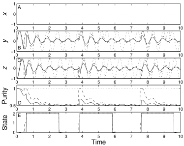
Figure 6: A typical trajectory for direct detection. The states attached to the TLA are plotted for a perfect observer (dotted lines), an intermediate observer who can monitor the detector transitions (dashed line) and a realistic observer who knows only when the avalanche reaches a threshold (solid line). In plot (E) the occupation probabilities for the various detector states are shown for the above trajectory, with the same legend applying. The closeness of the lines to the states $0$ and $1$ indicates the relative probability of occupation. The realistic parameters used for this photodetection trajectory are $\eta=80\%$, and (in terms of the TLA decay rate $\Gamma=300$M$s^{-1}$) $\gamma_{{\rm r}}=7\Gamma$, $\tau_{{\rm dd}}=2\Gamma^{-1}$, $\gamma_{{\rm dk}}=5\times 10^{-6}\Gamma$ and $\Omega=10\Gamma$.

When the atom jumps (here for the sake of simplicity, we will talk about the perfect trajectory as if that is what the TLA is actually doing) then the detector will only respond if it is in the ready state and if the photon absorption leads to the creation of a charged pair, which occurs a fraction $\eta$ of the time. At the time of the first TLA jump, the detector is almost certainly in the ready state (dark counts are negligible). From $y$ and $z$ in Fig. 6 (B) and (C) we see that the intermediate observer’s state responds immediately, while the realistic observer has to wait until an avalanche builds up before registering the detection. By this time, the TLA would no longer be in the ground state, so the jump does not take $z$ to $-1$ (or $y$ to $0$). In fact, the first avalanche actually increases $z$ for the realistic observer, contrary to naive expectations. This occurs because the response rate ($\gamma_{{\rm r}}=7$) is smaller than the driving strength ($\Omega=10$) for this trajectory. It is likely that the TLA will have been driven so that it is closer to the excited state than the ground state in the time taken for an avalanche to build up.

After a jump has occurred, the trajectories separate significantly. This is because the detector is ‘dead’ and provides no information about the TLA. The evolution during this time for the two non-perfect trajectories is via the unconditioned ME. The detector can register no more photons until it is restored to the ready state, a time $\tau_{{\rm dd}}$ after the avalanche has reached the threshold level.

It can be seen from Fig. 6 (D) that when a jump occurs, the intermediate observer’s state becomes pure (the impurity introduced by the dark counts is negligible). Obviously, this is because it is known that the TLA is the ground state, which is itself a pure state. By contrast, the realistic observer’s state has a purity of approximately $0.7$ after an avalanche. Apart from the first avalanche, this represents a purification. It arises because (incomplete) information has been gained about the time that the TLA most recently decayed into the ground state.

As the response rate $\gamma_{{\rm r}}$ of the detector is large compared to the photon flux of the TLA ($\approx\Gamma/2$ under perfect detection) the occupation probability of the ready state is close to unity for times after the detector has been restored to the ready state (see Fig. 6 (E)). That is, the transition rate out of state $1$ is considerably larger than the transition rate into this state. Another feature of the trajectories is that the $x$ quadrature remains at zero for all time, since the Hamiltonian is proportional to $\sigma_{x}$. Further details and the physical parameters used for the detector are included in the figure caption.

The method of simulating the three trajectories for direct detection was to firstly unravel the ME for the TLA according to perfect direct detection as in Eq. (6). Thus, a string of jump times at which $dN(t)=1$ was obtained, along with the trajectory for the perfect observer. The method of correlating the other two trajectories has already been given in Sec. IV.

IV.3 Adaptive Detection

To show how a realistic APD performs when monitoring the evolution of a TLA in a different way, we consider the adaptive detection scheme described in Sec. II.3. In realistic adaptive detection the LO amplitude will be flipped once the avalanche reaches threshold, as opposed to the case of perfect detection for which it is flipped at an earlier time corresponding to when the TLA decays. Thus, even the perfect trajectory will not exhibit two-state jumping if we flip the LO at the same delayed time for all the trajectories. This is done in order to stay as close as possible to how the experiment would be performed.

Trajectories for the same three observers as in direct detection are shown in Fig. 7. Looking at the $x$ quadrature, initially the three states head towards a particular eigenstate of the no-jump operator, then a jump occurs in the perfect and intermediate trajectories. A short time after this the realistic trajectory ‘avalanches’ and closely joins the other two. At this time the LO amplitude is flipped.

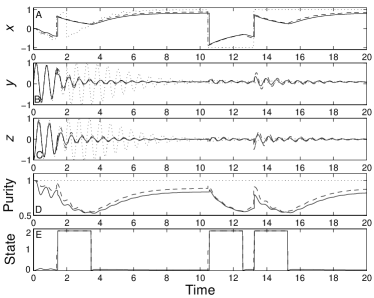
Figure 7: A typical trajectory for adaptive detection. The simulation parameters and legend are as for Fig. 6.

The TLA (in perfect detection) then closes in on the second no-jump evolution eigenstate, while the detector is ‘dead’. The non-perfect trajectories are evolving via the unconditioned ME, away from the eigenstate. The perfect trajectory then jumps away from the $x=1$ state, implying that a another photon has been detected in the combined TLA-LO field. If the LO were being controlled by the perfect trajectory, then at this point its amplitude would be flipped and the TLA would evolve towards the new eigenstate based on the new $\mu$. However, the LO is not ‘flipped’ as this photon goes undetected by the APD. The eigenstate of the no-jump evolution, therefore, does not change and the TLA in the perfect trajectory must evolve back towards it.

A time $\tau_{{\rm dd}}$ after the avalanche, the detector is ready again and the non-perfect states head towards that of the perfect trajectory. The next decay, which happens to be detected by the APD, takes all the states to the other side of the Bloch sphere.

The $y$ quadrature and $z$ in (B) and (C) display similar features when evolving via the ME or the no-jump operator. This is because the ME steady state and the operator steady state both have $y$ and $z$ close to zero, due to the large $\Omega$ being used. As time progresses, the three observers’ states head towards the steady states, thus reducing the $y,z$ oscillation amplitude.

One can see from (D) that the purity decreases significantly when the APD is dead and unconditioned ME evolution is occurring. When it is restored to the ready state, the purity increases as no matter where the TLA is in the Bloch sphere, it will head towards the no-jump evolution eigenstate. The average purity is substantially higher than for direct detection. This will be discussed later, when we consider system averages. Another point is that there is less difference between the purity of the trajectories of the intermediate and realistic observers. This is because the state of the TLA is not as sensitive as direct detection to the time of emission. The $\Omega$ dynamics that quickly ‘swept’ the TLA state away from the ground state before the realistic trajectory jumped are not present in adaptive detection.

The simulations of the adaptive trajectories are more difficult than those of direct detection, as the perfect trajectory cannot be run first to determine the decay times. This is because the evolution of the TLA depends on the LO amplitude, which is dependent upon the realistic trajectory. However, deciding the jump times of the perfect trajectory from those of the realistic trajectory is difficult. The best way to do the simulations is to run them in ‘parallel’ so that all three trajectories are being evolved at the same time. The perfect trajectory evolves under the LO determined by the realistic trajectory, but the avalanches of the realistic trajectory are determined by the jumps of the perfect trajectory in the same manner as direct detection. When the APD avalanches the LO is inverted for all three trajectories.

IV.4 Average Conditional Purity

So far we have shown only typical features of realistic detection and how they differ from perfect detection. In this section we quantify this difference by considering the steady state average purity of the conditional TLA state. This is defined as

$$p=\lim_{t\to\infty}{\rm E}\left\{{{\rm Tr}[\rho_{\rm c}^{2}(t)]}\right\},$$ (20)

where the c subscript is included to emphasize that $\rho_{\rm c}$ is a conditional state. Because purity is a nonlinear function of $\rho$ (2), the steady state ensemble average of the conditional purity is not the same as the purity of the steady state ensemble average, which is Eq. (5). The quality factor $p$ will be less than one, but always greater than $1/2$. The effect of the detector imperfections can be seen by comparing $p$ for the different measurement schemes and for a range of driving strengths, $\Omega$.

For small $\Omega$, even the unconditioned (without measurement) stationary purity $p_{\rm ME}$ of the TLA approaches unity. To distinguish better detection schemes in this limit it is useful to define a scaled purity (between $0$ and $1$) that measures how much improvement measurement produces:

$${\rm Scaled\;}p=\frac{p-p_{{\rm ME}}}{1-p_{{\rm ME}}}.$$ (21)

For perfect detection the conditional purity is always 1, so the scaled $p$ equals 1 also. For no measurement (master equation evolution), the scaled $p$ equals 0.

In Fig. 8 we plot the ensemble averaged purity (and scaled purity) as a function of the TLA driving strength, $\Omega$, for realistic detection, direct and adaptive. The trends in this figure result from two main imperfections, the dead time and the response time.

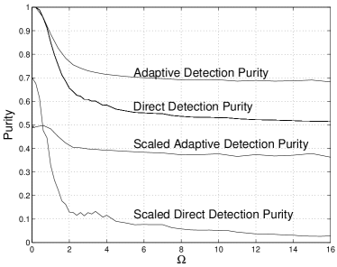
Figure 8: The (scaled and unscaled) ensemble averaged conditional purity for realistic direct and adaptive detection as a function of the TLA driving strength, $\Omega$ (in units of $\Gamma$). Detector parameters are as for Fig. 6. In this, and subsequent similar plots, the unevenness in the lines is due to, and indicates the size of, statistical error.

First consider the input photon flux in each of the two schemes, given in Eqs. (7)–(8). At low $\Omega$, direct detection produces purer conditioned states. This is because in this regime $f_{{\rm direct}}<f_{{\rm adapt.}}$, and direct detection is therefore less subject to having detections ‘missed’ due to the dead time $\tau_{\rm dd}$. As $f_{\rm direct}$ increases with $\Omega$, direct detection becomes worse than adaptive detection as $f_{\rm direct}$ surpasses $f_{\rm adapt.}$.

Note, however, that $f_{\rm direct}$ saturates at $\Gamma/2$, but the scaled purity for direct detection continues to decrease as $\Omega$ increases. This is due to the finite detector bandwidth. Under direct detection, the conditioned state of the TLA Rabi cycles at rate $\Omega$ (see Fig. 6). The response time $\gamma_{\rm r}^{-1}$ can be thought of as the uncertainty in the time of photoemission from the TLA, given an avalanche. For $\Omega\sim\gamma_{\rm r}$, the TLA state conditioned on a detection is ‘smeared out’ by the consequent uncertainty in how far the Rabi cycling has taken the atom from the ground state since its emission. By contrast, under adaptive detection, the scaled purity asymptotes to a nonzero value because the conditioned dynamics are governed by $\Gamma$, not $\Omega$ WisToo99 (see Fig. 7). Thus the adaptive purity levels off for high $\Omega$. From Fig. 8, the difference in the purity of the trajectories shown for direct and adaptive detection is quite large for $\Omega=10$, as expected from the trajectories shown in Figs. 6 and 7.

V Conditioned Dynamics For Homodyne Detection

For the PR, three different levels of ‘realism’ will be considered, as for the APD. The first observer once again has the ‘perfect’ measurement record. This record is the photon flux incident upon the p-i-n photodiode. The evolution of this observer’s state is via Eq. (9).

The intermediate observer has detailed access to the circuit containing the transimpedance amplifier and is able to determine $I$ and $V$ (see Fig. 4 in the preceding paper). This means, however, that this observer is still subject to the diode inefficiency. The current $I$ is given by

$$I=e\sqrt{{\rm P}/\hbar\omega_{0}}\left[\eta\langle e^{-i\Phi}c+e^{i\Phi}c^{{\dagger}}\rangle+\sqrt{\eta}\,\xi^{\prime}(t)\right],$$ (22)

where the parameters are explained in Sec. IV of the preceding paper. The SME for conditioning upon this current is

$$d\rho_{I}=dt\left\{{\cal L}+\sqrt{\eta}\,\xi^{\prime}(t){\cal H}[e^{-i\Phi}c]\right\}\rho.$$ (23)

The white noise $\xi^{\prime}(t)$ in the above equations is related to $\xi(t)$ in Eq. (9) by

$$\xi^{\prime}(t)=\sqrt{\eta}\,\xi(t)+\sqrt{1-\eta}\,\zeta(t).$$ (24)

This is due to the noise arising from two independent sources: the Poisson statistics of the LO and the vacuum noise introduced by the inefficiency of the photodiode.

To relate this to the realistic observer, we use for the capacitor voltage

$$\dot{V}^{\prime}=-\frac{V^{\prime}}{RC}-\frac{I}{C},$$ (25)

or, in terms of the scaled voltage,

$$\dot{v}^{\prime} = -\gamma v^{\prime}-\sqrt{\frac{\gamma}{N}}\left[\phantom{\sqrt{1-\eta}}\!\!\!\!\!\!\!\!\!\!\!\!\!\!\!\!\!\!\!\sqrt{\eta}\,\left\langle{e^{-i\Phi}c+e^{i\Phi}c^{{\dagger}}}\right\rangle+\sqrt{\eta}\xi(t)\right.$$ (26)

$$\left.\phantom{+\sqrt{1-\eta}\zeta(t)}+\sqrt{1-\eta}\zeta(t)\right].$$

Here, $V^{\prime}$ represents the unscaled true capacitor voltage. A prime is used to distinguish it from the argument (dummy variable) of the probability distribution used by the realistic observer. The expectation value in Eq. (26) is based on the state matrix obtained through perfect detection.

The realistic observer will have access to the output voltage ${\cal V}$ measured in the laboratory. The evolution of this observer’s state is via the SKSE for $\rho(v)$:

$$d\rho_{{\cal V}}(v) = dt\left({\cal L}+\frac{\gamma}{2N}\frac{\partial^{2}}{\partial v^{2}}+\gamma\frac{\partial}{\partial v}v\right)\rho(v)$$ (27)

$${+}\,dt\frac{\partial}{\partial v}\sqrt{\frac{\gamma\eta}{N}}\left[e^{-i\Phi}c\rho(v)+e^{i\Phi}\rho(v)c^{{\dagger}}\right]$$

$$+\sqrt{\gamma}\,d{\cal W}_{{\rm J}}(t)\left(v-\langle v\rangle\right)\rho(v).$$

For simulating the realistic trajectory alone, $d{\cal W}_{{\rm J}}(t)$ would be chosen to be an infinitesimal Wiener increment. However, to make it consistent with the perfect and intermediate observers, we must use the following relation from the preceding paper.

$$\sqrt{\gamma}\,d{\cal W}_{{\rm J}}(t) = dt\gamma\left({\sqrt{\frac{C}{4k_{\rm B}T}}\,{\cal V}-\left\langle{v}\right\rangle}\right)$$ (29)

$$= dt\gamma\sqrt{\frac{C}{4k_{\rm B}T}}\,\left(V^{\prime}+\sqrt{4k_{{\rm B}}TR}\frac{dW_{{\rm J}}(t)}{dt}\right)$$

$${-}\,dt\gamma\left\langle{v}\right\rangle$$

$$= \sqrt{\gamma}\,dW_{{\rm J}}(t)+dt\gamma\left({v^{\prime}-\left\langle{v}\right\rangle}\right).$$ (30)

Here $dW_{{\rm J}}(t)$ is due to the ‘real’ Johnson noise, and is generated as an infinitesimal Wiener increment. Thus $v^{\prime}$ correlates the equation for the realistic observer with those for the other two.

Simulation of the three correlated trajectories for homodyne detection was done in parallel, similarly to adaptive detection. This avoids the necessity of storing the photon flux and $\left\langle{e^{-i\Phi}c+e^{i\Phi}c^{{\dagger}}}\right\rangle$ from the perfect trajectory at every time step, for later use in the realistic trajectories. Once again the reader should see Sec. VII for some of the computer programming details.

V.1 Parameter Values for the Photoreceiver

The same quantum system is monitored as in the case of photon counting (with $\Gamma=300{\rm Ms^{-1}}$). For the PR, we chose values $\gamma=450{\rm Ms^{-1}}$, $N=0.1$ and $\eta=0.98$. These are reasonable values for detectors in quantum optics laboratories MabPriv . Note that the efficiencies for the photodiodes of PRs are much higher than those of APDs. This is because there are various difficulties in ensuring that photon absorptions lead to avalanches. Merely sweeping the single charged-pair out of the depletion region is an easier task.

There is generally a trade-off between bandwidth $\gamma$ and the dimensionless noise level $N$ MabPriv . We have chosen a relatively low noise level, and consequently a bandwidth below the maximum available. This noise level can be related to the (more usually quoted) noise equivalent power (NEP) as follows. Consider for specificity the PR model#2007 found in the New Focus catalogue newFoc . This model has a (NEP) of $\sim 3{\rm pW}/\sqrt{{\rm Hz}}\,$ (but a bandwidth of only $790{\rm kHz}$). The NEP can be interpreted as the extra optical power that would need to be injected into the receiver to simulate noise. To obtain $N$ from the NEP, we must compare it to the LO shot noise that is incident in homodyne detection. If the LO has transmitted power of ${\rm P}$ then in a time interval $\delta t$ the size of the photon number fluctuation will be $\sim\sqrt{{\rm P}\delta t/\hbar\omega_{0}}\,$. The NEP, on the other hand, will produce about $({\rm NEP}\hbar\omega_{0})\sqrt{\delta t}\,$ photons. Thus, $N={\rm NEP}/\sqrt{{\rm P}\hbar\omega_{0}}\,$. For this PR working close to saturation, ${\rm P}\approx 0.5{\rm mW}$ newFoc , so that $N\approx 0.1$ for a $\lambda=780{\rm nm}$ LO.

V.2 Homodyne $x$ Detection

Trajectories for homodyne detection of the $x$ quadrature ($\Phi=0$) are given in Fig. 9. The line-type allocations are as for photodetection: dotted is perfect, dashed is the intermediate observer and solid is the realistic trajectory. The perfect trajectory has been described in Sec. II.4.

See attached file HomX.jpg

Figure 9: A typical trajectory for homodyne $x$ detection. The states attached to the TLA are plotted for a perfect observer (dotted lines), an intermediate observer who knows the capacitor voltage $V$ (dashed line) and a realistic observer who knows only the output voltage ${\cal V}$ (solid line). Note that at some times the dotted and dashed lines are overlapping. In plot (E) the occupation probabilities for the scaled capacitor voltage ($v$) are given in a grey scale plot. Darker voltages are more likely. The PR parameters are $N=0.1$, $\eta=98\%$, $\gamma=1.5\Gamma$. System parameters are as for Fig. 6.

Because the photodiodes of PRs have a high efficiency (taken to be $\eta=0.98$), the trajectories for perfect and intermediate detection are very close, especially in $y$ and $z$. The Johnson noise and response time of the circuit make it more difficult for the realistic observer to follow the TLA state, although a similar trajectory is still obtained. The smaller detail of the perfect trajectory is mostly lost as the realistic observer has trouble identifying LO fluctuations that have been filtered and then obscured by Johnson noise. Another feature is that the realistic trajectory never gets as close as the perfect trajectory to being in an $y$ or $z$ eigenstate, reflecting the mixed nature of the state.

¿From the final subplot (E) of Fig. 9, it can be seen that to some extent the distribution for the scaled capacitor voltage follows the value of $x$, as one would expect since the current is proportional to $x$. Note that the purity dips whenever there is a large fluctuation in the $x$ trajectory. This is indicative of quicker evolution being more difficult to follow.

V.3 Homodyne $y$ Detection

The trajectories for homodyne detection of the $y$ quadrature ($\Phi=-\pi/2$) are given in Fig. 10. Once again Sec. II.4 should be referenced for brief comments on the perfect trajectory. For homodyne $y$ measurement the trajectory associated with inefficient detection is close to that of perfect detection, as it was for the homodyne $x$ measurement. The realistic trajectory is a reasonable approximation to the general shape of the perfect trajectory, although the $y$ quadrature is not being as closely followed as the $x$ quadrature was for the $x$ measurement. Note that the amplitude of oscillation of $y$ and $z$ is reduced for realistic detection.

See attached file HomY.jpg

Figure 10: A typical trajectory for homodyne $y$ detection. Legend and parameters are as for Fig. 9

The distribution for the detector state is influenced by $y$, but oscillations are barely visible. The purity in (D) is lower than the purity for homodyne $x$ measurement, due the faster evolution of the TLA being more difficult to follow. This will now be discussed in more detail.

V.4 Average Conditional Purity

In this section we investigate the long-time ensemble averaged conditional purity $p$ as a function of the driving strength for the PR. Homodyne measurement of the $x$ and $y$ quadratures of the TLA are contrasted.

The results in Fig. 11 indicate that as $\Omega$ increases, homodyne measurement of the $y$ quadrature becomes increasingly worse at following the evolution of the TLA. This is due to the finite bandwidth of the PR in combination with the conditional homodyne dynamics in the $\Omega\gg\Gamma$ limit WisMil93c . Homodyne $y$ detection produces a conditional state whose evolution is dominated by fast ($\Omega$) Rabi cycling (see Fig. 10). This is because $x$ is strictly zero, leaving only the $\Omega$ dependent $y$ and $z$ in the expression for $\rho$.

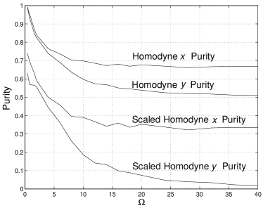
Figure 11: The long-time ensemble averaged purity and scaled purity is shown for realistic homodyne $x$ and $y$ detection as a function of the TLA driving strength, $\Omega$. Detector parameters are as for Fig. 9.

By contrast, homodyne $x$ detection produces mainly slow ($\Gamma$) dynamics, which can still be tracked by the detector (see Fig. 9). The homodyne $x$ measurement pushes $x$ towards the eigenstate ($\pm 1$), which means that $y$ and $z$ must be considerably less than unity as $x^{2}+y^{2}+z^{2}\leq 1$. The state is, therefore, dependent strongly on $x$, which is devoid of $\Omega$ oscillation. This explains why increasing $\Omega$ beyond a certain point does not cause further loss of purity under $x$ detection. These differences are seen more clearly in the scaled purity.

VI Effective Photoreceiver Bandwidth

In Sec. IV B of the preceding paper we presented the argument that for small electronic noise $N\ll 1$, the effective bandwidth $B$ of a PR is given not by $\gamma=1/RC$, but rather by

$$B=\gamma\sqrt{\frac{1-N}{N}}\simeq\frac{\gamma}{\sqrt{N}}.$$ (31)

The meaning of $B$ is that we expect the realistic trajectories from the PR to be unable to track system dynamics which have a rate much larger than $B$. In this section we investigate this claim by studying the realistic quantum trajectories for two very different systems. The first is the TLA we have used as our model system so far. The second is the DPOBT.

VI.1 Two-Level Atom

To test the prediction of the effective bandwidth the ensemble purity of the TLA was calculated for a range of $\gamma$ and $N$, while maintaining the proposed quality indicator of the PR, $\gamma\sqrt{1-N}/\sqrt{N}$, as a constant. Our theory predicts that the purity will remain constant. The results for homodyne $x$ measurement are contained in Fig. 12 and show that the purity is indeed relatively flat, when it is considered that $N$ is varying by almost two orders of magnitude.

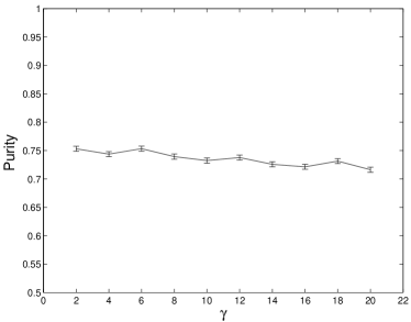
Figure 12: The ensemble averaged purity as a function of $\gamma$ for realistic homodyne $x$ detection when $\gamma\sqrt{1-N}/\sqrt{N}$ is kept constant at a value of $20$. The efficiency is $\eta=98\%$ and the driving strength of the TLA is $\Omega=30$. Error bars are included to make it clear that the slight downward slope is not due to fluctuations.

There is nevertheless a slight downward trend in the graph in Fig. 12. This is most likely due to the presence of increased noise as $\gamma$ (and $N$) increases. As explained in the preceding paper, our argument only makes sense for small $N$. In the limit of $\gamma\rightarrow\infty$ we are returning to the situation of adding noise only (discussed in the preceding paper), which is equivalently described by an inefficiency of $\eta/(1+N)$. Thus even if $B\to\infty$ as $\gamma\to\infty$, a finite noise $N$ would still reduce the system purity.

If $B$ could be kept constant with $N$ decreasing to zero then we would expect our prediction to become exact. Unfortunately this is a difficult regime to test numerically as it is actually the ratio of $\gamma/N$ not $\gamma/\sqrt{N}$ that appears in Eq. (27). With $\gamma,N\rightarrow 0$, but $B$ constant, $\gamma/N\rightarrow\infty$. The time step involved in the simulation decreases and the number of iterations of Eq. (27) increases, causing the computational intensity to become prohibitive (see Sec. VII).

Further support for identifying $B$ with the effective bandwidth is found in Fig. 11, where purity and scaled purity are plotted against $\Omega$. It is expected that approximately half the total loss of purity will have occurred once $\Omega\sim B$. That is, once the frequency of the monitored signal becomes equal to the effective inverse response time of the receiver. With the parameters of Fig. 11 we have $\gamma\sqrt{1-N}/\sqrt{N}=4.5$, which is in approximate agreement with the value of $\Omega$ such that $p=(p_{{\rm max}}+p_{{\rm min}})/2$. Only approximate agreement is expected because of the complicating issue of noise, as discussed previously.

VI.2 Degenerate Parametric Oscillator

Although the TLA is a small system, amenable to numerical simulations, it is usually not possible to find analytical solutions for its quantum trajectories. This is true of perfect detection schemes, let alone realistic detection schemes. We have seen above that even numerically it is difficult to do simulations in a regime of theoretical interest, $\gamma,N\to 0$ such that $B$ is finite. For this reason, we now turn to a simpler quantum system, the degenerate parametric oscillator below threshold.

The DPOBT system consists of a damped single-mode optical cavity containing a $\chi^{(2)}$ nonlinear crystal which is pumped by a (classically described) laser at twice the cavity frequency. We take the intensity damping rate to be unity and the parametric driving strength, $\chi$, to be of modulus less than unity. This leads to squeezing in the $y$ quadrature, $-i(a-a^{{\dagger}})$, if $\chi>0$ and squeezing in the $x$ quadrature, $a+a^{{\dagger}}$, if $\chi<0$. The system obeys the following ME

$$d\rho=dt\left(-\mbox{$\frac{1}{4}$}\chi[a^{2}-a^{{\dagger}2},\rho]+{\cal D}[a]\rho\right),$$ (32)

when no measurement is performed.

We will limit ourselves to considering realistic homodyne measurement of the $x$ quadrature. Using Eq. (27) with $c=a$, the SKSE is

$$d\rho_{{\cal V}}(v) = dt\left(-\mbox{$\frac{1}{4}$}\chi{\cal H}\left[a^{2}-a^{{\dagger}2}\right]+{\cal D}[a]\phantom{\frac{\partial^{2}}{\partial v^{2}}}\right.$$ (33)

$$\left.\phantom{+{\cal D}[a]+{\cal D}[a]}+\frac{\gamma}{2N}\frac{\partial^{2}}{\partial v^{2}}+\gamma\frac{\partial}{\partial v}v\right)\rho(v)$$

$$+\frac{\partial}{\partial v}\sqrt{\frac{\gamma\eta}{N}}\left[a\rho(v)+\rho(v)a^{{\dagger}}\right]$$

$$+\sqrt{\gamma}\,d{\cal W}_{{\rm J}}(t)\left(v-\langle v\rangle\right)\rho(v).$$

The superoperator can be removed by converting this into a Kushner-Stratonovich equation (KSE) for the probability distribution, $P(x,v)$, for $x$ and $v$. This is done using the standard procedure for Wigner functions presented in Ref. GarNoise . The distribution is defined by

$$P(x,v)=\langle{x}|\rho(v)|{x}\rangle,$$ (34)

with $|{x}\rangle$ being an eigenstate of the $x$ quadrature operator. Due to the linear nature of the optical cavity the measurement of the $x$ quadrature does not disturb the distribution for the $y$ quadrature after initial transients have died away. Thus, all statistics concerning the $y$ quadrature can be obtained from the unconditioned ME. In particular, the variance of the $y$ quadrature, $\Delta_{y}$, in the steady state of the ME is

$$\Delta_{y}=\frac{1}{(1+\chi)^{2}}.$$ (35)

Conversion of Eq. (33) gives

$$dP_{{\cal V}}(x,v) = dt\left[k\frac{\partial}{\partial x}x+\frac{1}{2}\frac{\partial^{2}}{\partial x^{2}}+\frac{\gamma}{2N}\frac{\partial^{2}}{\partial v^{2}}+\right.$$ (36)

$$\left.\gamma\frac{\partial}{\partial v}v+\sqrt{\frac{\gamma\eta}{N}}\frac{\partial}{\partial v}\left(x+\frac{\partial}{\partial x}\right)\right]P(x,v)$$

$${+}\,\sqrt{\gamma}\,d{\cal W}_{{\rm J}}(t)\left(v-\langle v\rangle\right)P(x,v),$$

where, $k=\mbox{$\frac{1}{2}$}(1-\chi)$, and the expectation value is found from

$$\left\langle{v}\right\rangle=\int dxdv\>vP(x,v).$$ (37)

The damping term has turned into drift and diffusion in $x$, while the parametric driving has become a drift term. It should be noted that in this section we are using $x$ to represent the possible values that the $x$ quadrature can take, rather than being the mean of the quadrature, which will be denoted by $\left\langle{x}\right\rangle$.

Despite its nonlinear and stochastic nature, a SKE of the form of Eq. (36) has analytical long-time solutions, a fact which is at the heart of modern engineering control techniques Jac93 . These solutions are Gaussians, and a closed set of equations of motion exist for the conditioned mean vector and covariance matrix for $x$ and $v$. The equation for the covariance matrix does not depend on the mean vector, and is also deterministic, thus having a steady state solution. We denote the three elements of the covariance matrix

$$\Delta_{x} = \left\langle{x^{2}}\right\rangle-\left\langle{x}\right\rangle^{2},$$ (38)

$$\Delta_{v} = \left\langle{v^{2}}\right\rangle-\left\langle{v}\right\rangle^{2},$$ (39)

$$\Delta_{xv} = \left\langle{xv}\right\rangle-\left\langle{x}\right\rangle\left\langle{v}\right\rangle.$$ (40)

It is important to remember the “Itô correction” Gar85 in calculating the equation of motion for these quantities. For example,

$$d\Delta_{x}=d\left\langle{x^{2}}\right\rangle-2\left\langle{x}\right\rangle d\left\langle{x}\right\rangle-d\left\langle{x}\right\rangle d\left\langle{x}\right\rangle.$$ (41)

Using integration by parts and the vanishing of $P(x,v)$ at infinity yields

$$d\left\langle{x}\right\rangle = -k\left\langle{x}\right\rangle dt+\sqrt{\gamma}d{\cal W}_{{\rm J}}(t)\Delta_{xv}$$ (42)

$$d\left\langle{v}\right\rangle = -\left(\gamma\left\langle{v}\right\rangle+\sqrt{\frac{\gamma\eta}{N}}\left\langle{x}\right\rangle\right)dt+\sqrt{\gamma}d{\cal W}_{{\rm J}}(t)\Delta_{v}$$

$$d\Delta_{x} = (-2k\Delta_{x}+1-\gamma\Delta_{xv}^{2})dt$$ (44)

$$d\Delta_{v} = \left(\frac{\gamma}{N}-2\sqrt{\frac{\gamma\eta}{N}}\Delta_{xv}-2\gamma\Delta_{v}-\gamma\Delta_{v}^{2}\right)dt$$ (45)

$$d\Delta_{xv} = -\left[(k+\gamma)\Delta_{xv}+\phantom{\sqrt{\frac{\gamma\eta}{N}}}\right.$$ (46)

$$\left.\phantom{\Delta_{xv}}\sqrt{\frac{\gamma\eta}{N}}\left(\Delta_{x}-1\right)+\gamma\Delta_{v}\Delta_{xv}\right]dt,$$

which are examples of Kalman filter equations KMan . In the long time limit the covariances are constant, and the whole distribution is just being shifted with the motion of the mean.

Since the purity of the cavity mode is defined in terms of the variances of the $x$ and $y$ quadratures, after initial transients have died the purity will be constant in time. For Gaussian states with no correlation between the $x$ and $y$ quadrature, the purity ${\rm Tr}[\rho^{2}]$ is given by HowVac

$$p=\frac{1}{\sqrt{\Delta_{x}\Delta_{y}}\,}.$$ (47)

There is an analytical steady state solution of Eqs. (44)–(46), but it is very complex and will not be given here. We are really only interested in the purity in the limit of small $N$ with $B=\gamma/\sqrt{N}$ fixed. If $B$ is indeed the effective bandwidth, as we have argued, then in the limit $N\to 0$ with $B$ fixed, the purity should depend on $B$ only, not $\gamma$ or $N$.

To show this we will examine Eqs. (44)–(46) more closely. The first step is to determine how $\Delta_{x},\Delta_{v},\Delta_{xv}$ scale as $\gamma,N\rightarrow 0$. Re-writing Eqs. (44)–(46) in terms of $B$ and $N$, we have from Eq. (44) at steady state

$$\Delta_{x}=\frac{1-B\sqrt{N}\Delta^{2}_{xv}}{2k}.$$ (48)

¿From the unconditioned ME, $\Delta_{x}$ would be $1/2k$, while we expect (and have verified numerically) that a finite $B$ will give a finite variation of the purity away from $p_{{\rm ME}}$. For this to be the case it must be true (when $\gamma,N\rightarrow 0$) that $\Delta_{x}\lesssim 1/2k$ with

$$B\sqrt{N}\Delta^{2}_{xv}\sim\sqrt{N}\Delta^{2}_{xv}\sim 1\;\Longrightarrow\;\Delta_{xv}\sim{N^{-1/4}}.$$ (49)

Ignoring the $\gamma$ term in Eq. (46) that is small compared to $k$ gives

$$\Delta_{v} = -\left[\frac{k}{B\sqrt{N}}+\frac{1}{\Delta_{xv}N^{3/4}}\sqrt{\frac{\eta}{B}}\left(\Delta_{x}-1\right)\right]$$ (50)

$$\sim N^{-1/2},$$

where we have used Eq. (49).

New variances of order unity are now defined:

$$\tilde{\Delta}_{v} = N^{1/2}\Delta_{v}$$ (51)

$$\tilde{\Delta}_{xv} = N^{1/4}\Delta_{xv}.$$ (52)

The variance in $x$ is kept the same, as it is of the order unity. Using these in Eqs. (44)–(46) and ignoring small terms allows these equations at steady state to be written as

$$-2k\Delta_{x}+1-B\tilde{\Delta}_{xv}^{2} = 0$$ (53)

$$B-2\sqrt{B\eta}\tilde{\Delta}_{xv}-B\tilde{\Delta}^{2}_{v} = 0$$ (54)

$$-k\tilde{\Delta}_{xv}-\sqrt{B\eta}(\Delta_{x}-1)-B\tilde{\Delta}_{xv}\ \tilde{\Delta}_{v} = 0.$$ (55)

Importantly, these equations, which apply in the $\gamma,N\rightarrow 0$ limit, are only dependent upon the detector parameters $B$ and $\eta$. This means that the $\gamma,N$ dependence of the purity can be summarized by the one parameter $B=\gamma/\sqrt{N}$. This confirms the correctness of our argument.

As Eqs. (53)–(55) are more simple than Eqs. (44)–(46) it would be useful to solve for $\Delta_{x}$, and hence purity. This can be done, using the facts that the variances are positive and that $\Delta_{x}\Delta_{y}\geq 1$ to discard non-physical solutions. The result for purity is

$$p=\left({\frac{{2k\eta(1-k)B^{2}}}{{S\sqrt{\eta B^{3}}\left(BR+k^{2}\right)-k^{4}-B^{2}k^{2}\left(1-\frac{\eta}{k}+\frac{2R}{B}\right)}}}\right)^{1/2},$$ (56)

with

$$R = \sqrt{k^{2}+\eta(1-2k)}$$

$$S = k\sqrt{\left({2BR+k^{2}+B^{2}}\right)/{\eta B^{3}}}.$$ (57)

We can now consider the two obvious limits of $B\rightarrow 0,\infty$ (with $\eta=1$ for simplicity). For $B\rightarrow 0$ the purity is, to lowest order in $B$,

$$p=p_{{\rm ME}}+\frac{B^{2}}{4}\frac{(1-2k)^{2}(1+k)^{2}}{k^{7/2}(1-k)^{3/2}}.$$ (58)

As $B\rightarrow\infty$ the purity to first order in $1/B$ is

$$p=1-\frac{1}{4B}\frac{(1-2k)^{2}}{(1-k)}.$$ (59)

That is, for small $B$, the purity increases from the unconditioned purity quadratically with the effective bandwidth, while for large $B$ it decreases from unity linearly in $B^{-1}$.

As a final point, it is worth noting that the downward trend observed in the purity in Fig. 12 for the TLA is also borne out in the DPOBT. That is, for fixed $B=\gamma\sqrt{1-N}/N$, the purity still has a slight downward trend with $N$. This was found through numeric investigation of the complete solution for the purity (which was not stated due its complexity). However, the numeric investigation also revealed that as $N\to 0$ the purity curve maintains the same slope, going to the limits found analytically above.

VII Numerical Simulations Technique

Before concluding, we here comment explicitly upon the method of numerical simulation of the SKSE’s contained in this paper. Obtaining realistic trajectories from Eqs. (16)–(18) and Eq. (27) is obviously a non-trivial numerical exercise, even when they do not have to be correlated with the unrealistic trajectories of the perfect and intermediate observers. To set up the problem, the Quantum Optics toolbox for Matlab QOTool was used. This allowed easy formulation of the required quantum (super)operator expressions.

We represented the supersystem state with a long column vector and a square matrix, ${\bf L}$, was used to evolve it. That is,

$$d\left(\begin{array}[]{ll}\rho_{1}\\ \vdots\\ \rho_{s}\\ \vdots\end{array}\right)=dt{\bf L}\left(\begin{array}[]{ll}\rho_{1}\\ \vdots\\ \rho_{s}\\ \vdots\end{array}\right),$$ (68)

where

$$\rho_{s}=\left(\begin{array}[]{ll}\rho_{s,e}\\ \rho_{s,ge}\\ \rho_{s,eg}\\ \rho_{s,g}\end{array}\right).$$ (69)

The subscripts $e,g$ represent the ground and excited state of the TLA. The integer subscripts $s$ label detector states $s\in\mathbb{S}$. For the APD there are only three detector states, while for the PR the scaled capacitor voltage is discretized on a grid. The matrix ${\bf L}$ generates all the evolution on the RHS of Eqs. (16)–(18) and Eq. (27).

Because of the stochastic nature of the realistic trajectories, ${\bf L}$ cannot in general be formed in its entirety at the start of the simulation. In the case of the APD one can avoid this difficulty by using the unnormalized versions of Eqs. (16)–(18). These were given in WarWisMab01 . The stochasticity then enters via the comparison of the norm of the supersystem state to a random number in order to choose the avalanche times. For the PR, the nonlinear term (the expectation value, $\langle v\rangle$) is included in the evolution. This, in addition to the noise, $d{\cal W}_{{\rm J}}(t)$, means that the best that can be done is to create the ${\bf L}$ for all but the last term of Eq. (27). The last term is created every time step after the calculation of the expectation value.

The structuring of the numeric solution in this way (creating as much as possible of ${\bf L}$ before the iteration process begins) makes it very flexible. For example, a change in the nature of the Hamiltonian for the TLA could be easily achieved by creating the new superoperator in the Quantum Optics toolbox and thus obtaining a new ${\bf L}$. This is in contrast to the technique of deriving $\dot{x}_{s},\dot{y}_{s},\dot{z}_{s}$ equations and then evolving these numerically, as a new Hamiltonian would require a new derivation.

The obvious disadvantage with ${\bf L}$ is that it will be very sparse in general. This is overcome by reducing it to only the non-zero elements, with the aid of the find command in Matlab. Once the reduced matrix has been found it is written to a data file which is used as the input for a C++ program.

The C++ program then integrates the matrix equation 68 by looping through all the non-zero ${\bf L}$ elements and making the appropriate increments. The simple Euler technique of integration is used, by which is meant that the infinitesimal $d$ in Eq. (68) is replaced by the small but finite $\delta$. This method has well known instabilities, but is used by other workers in the field of quantum optics. It has the property of being accurate when the solutions do not explode, as opposed to more stable methods which have less spectacular failures that are more difficult to detect EulerCarmichael .

Some specific details of the PR simulations are as follows. A stationary grid of $100$ points was used for the capacitor voltage distribution. These points were spread $7$ standard deviations of the initial distribution either side of the initial mean. The initial distribution was found by solving the Ornstein-Uhlenbeck equation Gar85

$$dP(v)=dt\left(\frac{\gamma}{2N}\frac{\partial^{2}}{\partial v^{2}}+\gamma\frac{\partial}{\partial v}v\right)P(v).$$ (70)

This is derived from the SKSE (27) by removing the TLA and averaging over the realistic measurement. Ignoring the TLA is reasonable as the field from the TLA is of the same order as the vacuum field. This leads to a Gaussian solution with a variance of $\Delta_{v,{\rm u}}=1/2N$, giving a standard deviation of $2.24$ for $N=0.1$. The u subscript is to indicate that this is a variance unconditioned on measurement. From Figs. (9)–(10), it can be seen that the considered range of voltages was sufficient.

A moving grid for the voltage distribution was considered but not used in the end. This decision can be justified by calculating the conditioned variance of the voltage distribution in the case of a vacuum input. Unlike the calculation of the variance from the Ornstein-Uhlenbeck equation, the stochastic measurement term

$$\sqrt{\gamma}\,d{\cal W}_{{\rm J}}(t)\left(v-\langle v\rangle\right)P(v)$$ (71)

is now included. The variance goes to a steady state value, despite the stochasticity. The derivation of the conditioned variance, $\Delta_{v,{\rm c}}$, is performed in the same manner as in Sec. VI B, and the result is

$$\Delta_{v,{\rm c}}=\sqrt{1+\frac{1}{N}}\,-1.$$ (72)

This is always smaller than the unconditioned variance, $1/2N$. In fact, in the limit $N\rightarrow 0$

$$\frac{\Delta_{v,{\rm u}}}{\Delta_{v,{\rm c}}}=\frac{1}{2\sqrt{N}\,}.$$ (73)

In this limit the conditioned variance becomes much smaller than the unconditioned variance and a moving grid would save much numerical computation. This is because the number of grid points necessary to describe the non-zero probabilities at a particular time is much less than those required to describe the movement of the distribution over all time. However, for $N=0.1$ we have $\Delta_{v,{\rm u}}=2.16\Delta_{v,{\rm c}}$ and the saving is not very large. It is worth noting that a moving grid would not solve all the computational intensity of $\gamma/N\rightarrow 0$ as the problem of the decreasing required time step still exists.

For the PR, time steps of $\delta t=1\times 10^{-5}\Gamma^{-1}$ generally proved satisfactory, as did ensemble sizes of about $1000$ for forming averages. The time step for the APD can be increased by about an order of magnitude as there is no white noise. The ensembles actually took the form of a collection of samples of the supersystem state in one trajectory, taken at times separated by $\Gamma^{-1}$. This is large compared to the system correlation time . The equivalence of this time averaging to a many trajectories average has been established by Cresser Cresser .

VIII Conclusion

In this paper we have applied the theory of realistic quantum trajectories for photodetection derived in the preceding paper WarWis02a to realistic quantum optical situations. We investigated two systems. The first was a driven two-level system, which could be realized as a strongly coupled atom-cavity system, heavily damped though one cavity mirror. For this system we solved for the trajectories numerically. We looked at features of typical stochastic trajectories, as well as a figure-of-merit, the ensemble averaged conditional purity, for how well the system state is known. We considered four different detection schemes: direct and adaptive detection using an avalanche photodiode (APD), and $x$ and $y$ quadrature homodyne detection using a photoreceiver (PR). The second system was a below threshold degenerate optical parametric oscillator. The conditioned evolution for this could be solved analytically for homodyne detection using a photoreceiver.

The first significant result we found is that for realistic detector parameters and realistic systems there is a large difference between standard (idealized) quantum trajectories and realistic quantum trajectories. Even with inefficiencies and dead time included in the standard trajectories, the differences are marked. This is due to the effect of finite detector response times. For example, for the strongly driven two-level system, the average conditional purity under realistic direct detection was scarcely better than with no detection at all.

The second significant result we found was the amount of difference the detection scheme makes, even using the same detector. With the APD, the adaptive scheme gave (for most parameter regimes) far higher purity than direct detection. For the PR, homodyne $x$ detection (with a local oscillator in quadrature with the system driving field) gave a similarly better result than homodyne $y$ detection. With a perfect detector the choice of detection scheme of course makes no difference as the conditional purity would always be unity.

A final significant result we found was that for homodyne detection the PR bandwidth $\gamma$ is not the relevant parameter for determining the rates of system evolution that can be tracked. Instead, the effective bandwidth is $B=\gamma/\sqrt{N}$. Here $N$ is the ratio of electronic noise to vacuum noise, which has been assumed small (as required in quantum optics experiments). We verified this result numerically for the two-level system and analytically for the parametric system. We would expect this result to be generalizable to other sorts of detection scheme, as long as they involve filtering and the addition of white noise. Mesoscopic electronics is an obvious example, as discussed in the preceding paper.

All of these results are relevant to the area of quantum control. As explained in the introduction, since a conditional state is a representation of the observer’s knowledge about a system, it is by definition the optimal basis for controlling that system. For this to work, the observer must have an accurate model for the relation between the available information (the detector output) and the quantum system. That is precisely what a realistic quantum trajectory is. The large differences between standard and realistic quantum trajectories noted above means that the former would be a poor approximation to the latter in a control system. That is, a realistic quantum trajectory theory is necessary. The differential performance of different measurement schemes may also be significant, if one can choose the measurement scheme to be used in the control loop.

Finally, another area where realistic quantum trajectories would probably be needed is in the estimation of dynamical parameters for open quantum system from monitoring the outputs of such systems. This has been investigated for perfect detection in Refs. Mab96 ; GamWis01 . The loss of information resulting from realistic detector imperfections will be the subject of future work.

References

- (1) P. Warszawski and H.M. Wiseman, preceding paper.
- (2) P. Warszawski, H. M. Wiseman and H. Mabuchi, Phys. Rev. A 65, 023802 (2002).
- (3) J. Dalibard, Y. Castin and K. Mølmer, Phys. Rev. Lett. 68, 580 (1992).
- (4) H. M. Wiseman and G. J. Milburn, Phys. Rev. A 47, 1652 (1993).
- (5) H. M. Wiseman and G. E. Toombes, Phys. Rev. A 60, 2474 (1999).
- (6) H. J. Carmichael, S. Singh, R. Vyas and P. R. Rice, Phys. Rev. A, 39, 1200 (1989).
- (7) H. M. Wiseman, Quantum Semiclass. Opt 8, 205 (1996).
- (8) A. C. Doherty, S. M. Tan, A. S. Parkins, and D. F. Walls, Phys. Rev. A 60, 2380 (1999).
- (9) T. A. Brun, J. Finkelstein, and N. D. Mermin, Phys. Rev. A. 65, 032315 (2002).
- (10) C. M. Caves, C. A. Fuchs and R. Shack, Phys. Rev. A. 65, 022305 (2002).
- (11) P. R. Rice and H. J. Carmichael, IEEE J. Quantum Elect. 24, 1351 (1988); Q. A. Turchette, R. J. Thompson, and H. J. Kimble, Appl. Phys. B 60, S1 (1995).
- (12) H. Mabuchi, California Institute of Technology, private communication.
- (13) www.newfocus.com
- (14) C. W. Gardiner, Quantum Noise (Springer-Verlag, Berlin, 1991).
- (15) O. L. R. Jacobs, Introduction to Control Theory, (Oxford University Press, Oxford, 1993); P. Whittle, Optimal Control, (John Wiley & Sons, Chichester, 1996).
- (16) F. S. Schweppe, Uncertain Dynamical Systems (Englewood Cliffs, NJ: Prentice-Hall).
- (17) H. M. Wiseman and J. A. Vaccaro, Phys. Lett. A 250, 241 (1998).
- (18) S. Tan, Quantum Optics Toolbox for Matlab, Version 0.10 11-Jan-1999 (University of Auckland).
- (19) H. Carmichael, University of Oregon, private communication.
- (20) C. W. Gardiner, Handbook of Stochastic Methods (Springer, Berlin, 1985).
- (21) J. D. Cresser, “Ergodicity of Quantum Trajectory Detection Records” in Directions in Quantum Optics eds. H. J. Carmichael, R. J. Glauber and M. O. Scully (Springer, Berlin, 2001).
-
(22)
H. Mabuchi,
Quan. Semiclass. Opt. 8, 1103 (1996). - (23) J. Gambetta and H.M. Wiseman, Phys. Rev. A 64, 042105 (2001).