Spatial antibunching of photons with parametric down-conversion
Abstract
The theoretical framework behind a recent experiment by Nogueira et al. [Phys. Rev. Lett. 86, 4009 (2001)] of spatial antibunching in a two-photon state generated by collinear type II parametric down-conversion and a birefringent double-slit is presented. The fourth-order quantum correlation function is evaluated and shown to violate the classical Schwarz-type inequality, ensuring that the field does not have a classical analog. We expect these results to be useful in the rapidly growing fields of quantum imaging and quantum information.
pacs:
03.65.Ud,03.65.Ta, 42.50.DvI Introduction
As current technology advances, more and more attention is placed upon Quantum Mechanics to solve future problems. Furthermore, quantum systems are capable of performing some tasks more efficiently than classical systems chuang00 , drawing even more emphasis to quantum technologies. In particular, the fields of optical communication, optical imaging and optical information processing have been appended by the rapidly developing fields of quantum communication barbosa98 ; enk99 ; pereira00 , quantum imaging gatti99 ; abouraddy01 and quantum information processing chuang00 . Thus, the study of quantum phenomena promises to be a fruitful enterprise.
For many years researchers have studied the non-classical behavior of light, such as squeezing stoler70 ; stoler71 ; slusher85 and antibunching carmichael76 ; kimble76 ; kimble77 . However, most theoretical and experimental investigations deal with time variables only. That is, most treatments consider only one spatial mode. In a recent review article, Kolobov kolobov99 demonstrates that many quantum phenomena also occur when considering spatial variables of the electromagnetic field. Many areas of technology stand to benefit from the possible applications provided by such quantum phenomena.
An invaluable tool in these areas of research is the generation of entangled photons using parametric down-conversion burnham70 . The two-photon state of light exhibits non-separable behavior fonseca99a ; fonseca01 and has been used in nearly all quantum information schemes cabello01 .
Spatial antibunching was recently observed experimentally by Nogueira et al. nogueira01 using spontaneous parametric down-conversion (SPDC). In this article, we provide a theoretical background for the experiment reported in nogueira01 . Section II is dedicated to the general introduction of temporal and spatial antibunching. In section III we discuss the theoretical observation of spatial antibunching of photons using a two-photon entangled state produced by SPDC, as in nogueira01 . We close with some concluding remarks in section IV.
II Photon bunching and antibunching
It is well known that any state of the electromagnetic field that has a classical analog can be described by means of a positive nonsingular Glauber-Sudarshan distribution, which has the properties of a classical probability functional over an ensemble of coherent states. Because of this fact, the normally-ordered intensity correlation function for stationary fields must obey the following inequality mandel95 :
| (1) |
where stands for time and normal ordering. Photon density operators are defined as
| (2) |
where
| (3) |
is the annihilation operator for the mode with wave vector and polarization , is the unit polarization vector, is the quantization volume and .
Expression (1) is commonly written in the shorter form
| (4) |
where
| (5) |
Since the delayed photon coincidence detection probability is proportional to mandel95 , inequality (4) means that for the class of fields considered above, photons are detected either bunched or randomly distributed in time. Photon antibunching in time, characterized by the violation of (1), was predicted by Carmichael and Walls carmichael76 , Kimble and Mandel kimble76 , and was first observed by Kimble, Dagenais and Mandel in resonance fluorescence kimble77 .
In the space domain, the concept analogous to stationarity is homogeneity. For a homogeneous field, the expectation value of any quantity that is a function of position is invariant under translation of the origin mandel95 . In particular, on a plane surface normal to the propagation direction,
| (6) |
and
| (7) |
where is the transverse position vector, and
For homogeneous and stationary fields described by positive nonsingular distributions, the Schwarz inequality implies that
| (8) |
that is,
| (9) |
Analogously to what was concluded from inequality (4), for fields that admit classical stochastic models, inequality (9) implies that photons are detected either spatially bunched or randomly spaced in a transverse detection screen. Violation of (9) implicates the possibility of quantum fields exhibiting spatial antibunching. Spatial antibunching of photons has been predicted by some authors kolobov99 ; berre-rousseau79 ; klyshko82 ; bialynicka-birula91 ; kolobov91 .
III Spatial antibunching with down-conversion
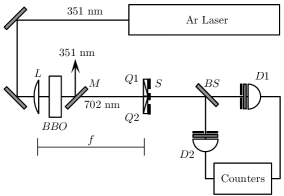
In this section we show that a field that violates inequality (9) can be generated by means of spontaneous parametric down-conversion. The experimental setup we are considering is shown in Fig. 2. A nonlinear birefringent crystal is used to generate collinear entangled photon pairs. The down-converted photons are then incident on a birefringent double-slit (see section III.1) and coincidences are detected by detectors and . The pump beam is focused on the center of the plane of the double-slit, between the two slits. Interference filters are used such that the monochromatic approximation is valid.
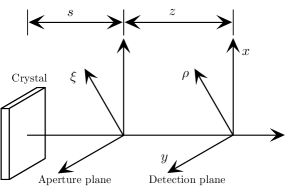
The following discussion refers to the basic geometry illustrated in Fig. 1, where a thin crystal is separated from an aperture plane by a distance and the aperture plane is separated from a detection plane by a distance .
Using a treatment based in reference hong85 , in the paraxial and monochromatic approximations, collinear SPDC generates a quantum state of the form monken98a :
| (10) |
with
| (11) |
The coefficients and are such that . depends on the crystal length, the nonlinearity coefficient, the magnitude of the pump field, among other factors. The kets represent Fock states labeled by the transverse component of the wave vector and the polarization of the down-converted photon . In this paper we consider type-II phase matching, in which case and where stands for extraordinary (ordinary) polarization. is the two-photon component of the total quantum state. The function , which can be regarded as the normalized angular spectrum of the two-photon field monken98a , is given by
| (12) |
where is the normalized angular spectrum of the pump beam, is the length of the nonlinear crystal in the -direction, and is the magnitude of the pump field wave vector. The integration domain is, in principle, defined by the conditions and . However, in most experimental conditions, the domain in which is appreciable is much smaller than that. The state written above is not to be considered as a general expression for the SPDC process. Its validity is determined by experimental conditions, especially by the detection apparatus. As long as the monochromatic and paraxial approximations are valid, the results predicted by expression (11) are in excellent agreement with experience. Monochromatic approximation is guaranteed by the presence of narrow-band interference filters in the detection apertures, whereas paraxial approximation is guaranteed by keeping transverse detection regions much smaller than their distance from the crystal.
We consider for now that the down-converted fields are incident on
some sort of aperture, so as to produce fourth-order interference in
the absence of second-order interference. The reason for such a
requirement is the following: Spatial photon antibunching is a
fourth-order effect in a homogeneous field, that is to say, in a field
that, according to 7, does not show intensity patterns.
With this scheme, we are seeking for a fourth-order interference
pattern that depends only on , the relative position of
detectors. Furthermore, this fourth-order interference pattern must
have a minimum when in order to produce antibunching.
Fourth-order spatial interference in the absence of second-order can
be achieved in spontaneous parametric down-conversion by means of a
double-slit whose slit separation is much greater than the transverse
coherence length of the down-converted field, as reported by Fonseca
et al. fonseca99 . However, in reference
fonseca99 the fourth-order correlation function, which is
proportional to the coincidence rate, depends on
instead of . In order to achieve a minimum of
coincidences when , we have to introduce a phase
difference of between the two possibilities
{photon 1 through
slit 1, photon 2 through slit 2} and {photon 1 through slit 2,
photon 2 through slit 1}. In our experiment, that phase difference
was introduced by means of birefringent elements placed in front of
each slit, as described later. After the aperture, the two-photon
state can be written as
| (13) | |||||
where is a normalization constant, is the angular spectrum of the biphoton field on the aperture plane, that is,
is the transfer function of the aperture, linking the incident field with transverse wave vector and polarization with the scattered field with transverse wave vector and polarization . is given by the Fourier transform of the aperture function .
Since we are working with collinear SPDC with , is written as
where the irrelevant phase factor is omitted.
Using the orthonormal properties of the Fock states, we can define
| (16) |
as the two photon coincidence detection amplitude, where
| (17) |
is the monochromatic form of (3) in the paraxial approximation and is the distance between the aperture plane and the detection plane, as shown in Fig. 1. It is assumed that the polarization vector is independent of . The two-photon coincidence-detection probability for stationary fields is proportional to the fourth-order correlation function with :
| (18) |
III.1 The birefringent double-slit
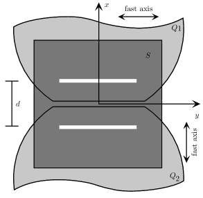
The birefringent double slit consists of two quarter-wave plates mounted in front of a typical double slit, such that each wave plate covers only one slit and their fast axes are orthogonal to one another, as shown in Fig. 3. The slits are separated a distance . With the plate-slit aperture oriented such that the slits and one fast axis are parallel to the () direction and the other fast axis parallel to the () direction, we can approximate the field-aperture functions by
| (19) |
where is the -component of . The plate-slit apertures provide a controlled phase factor, that is, no phase will be added to a field with polarization parallel to the direction of the fast-axis of the wave-plate, while a field with perpendicular polarization will be modified by a phase factor of . Thus, the phase factor depends on the polarization of the field as well as through which slit the field “passes”.
III.2 The coincidence-detection probability amplitude
Combining equations (13–17) and (19), we arrive at the following expression for coincidence-detection amplitude in the Fraunhofer approximation:
| (20) |
where
where the “” holds for and the “” holds for .
We assume that the pump field is a gaussian beam whose waist is located on the aperture plane:
| (22) |
Its angular spectrum is
| (23) |
where is the radius of the beam waist. Using (LABEL:eq:phia) and (23) in (LABEL:eq:detect), it is straightforward to show that
| (24) |
It is interesting to note that the length of the nonlinear crystal enters in the coincidence-detection amplitude only as a multiplicative constant. It is clear from expression (24) above, that the fulfillment of the homogeneity condition (7) for in the -direction depends on the factor . If , the dependence on disappears and transverse field on the detection plane can be considered as homogeneous. This is the reason why the pump beam must be focused on the center of the double slit. In this case,
| (25) |
Thus, the coincidence detection probability is
| (26) |
When , the coincidence count rate is zero and increases with until . Therefore, the fourth-order correlation function , which is proportional to the coincidence detection probability , does not have a maximum at . This contradicts (9), thus characterizing spatial antibunching of photons.
IV Discussion and conclusion
We have shown the theoretical background behind the spatial antibunching of photons using parametric down-conversion. It may be instructive for the reader to compare the experiment analyzed here with its classical counterpart. In this context, the single count detection rate should be proportional to the classical average intensity , whereas the coincidence count rate should be proportional to the intensity-intensity (or the fourth-order) correlation function . The single count detection rate of down-converted light in the presence of a double-slit has been studied in previous works fonseca99 ; ribeiro94 ; ribeiro99 . In reference ribeiro94 it was demonstrated that in terms of its single count rate, SPDC behaves like a classical Schell-model extended light source. In our experiment, the transverse coherence length being shorter than the slits separation and shorter than the slits widths themselves, the single count rate is given by the classical expression for incoherent illumination, which can be approximated by a gaussian
| (27) |
where and is the width of the slits. Since the transverse detection range is much shorter than the width of this gaussian profile for the slits-detectors distance considered, the single count rate is fairly constant over de detection range nogueira01 . By another side, the coincidence detection rate due to a classical source is totally different from the observed with down-converted light. Perhaps, the best classical model for type-II SPDC is a superposition of two extended light sources orthogonally polarized and correlated in intensity. After the light is diffracted by the birefringent double-slit, the calculation of the classical fourth-order correlation function is quite similar to the case of the Hanbury Brown – Twiss intensity interferometer hbt . Classical intensity interferometry is known to be insensitive to phase. Therefore, the birefringent elements have no effect on the predicted fourth-order correlation, that is,
| (28) |
The visibility is in the range and depends on the statistics of the source. It is clear from expression (28) above that predicts spatial bunching, as expected from any classical light source. In view of the above analysis, the results presented here describe an entirely quantum fourth-order interference effect, with no classical analog belinsky92 . In addition to rendering further interest in the study of non-classical states of light, spatial antibunching promises to be a useful tool in quantum imaging and quantum information technologies.
Acknowledgements.
The authors acknowledge financial support from the Brazilian agencies CNPq and CAPES.References
- (1) M. A. Nielsen and I. L. Chuang, Quantum Computation and Quantum Information (Cambridge, Cambridge, 2000).
- (2) G. A. Barbosa, Phys. Rev. A 58, 3332 (1998).
- (3) S. J. van Enk, H. J. Kimble, J. I. Cirac and P. Zoller, Phys. Rev. A 59, 2659 (1999).
- (4) S. F. Pereira, Z. Y. Ou and H. J. Kimble, Phys. Rev. A 62, 042311 (2000).
- (5) A. Gatti, E. Brambilla, L. Lugiato and M. I. Kolobov, Phys. Rev. Lett. 83, 1763 (1999).
- (6) A. F. Abouraddy,B. E. A. Saleh, A. V. Sergienko and M. C. Teich, Phys. Rev. Lett. 87, 123602 (2001).
- (7) D. Stoler, Phys. Rev. D. 1, 3217 (1970).
- (8) D. Stoler, Phys. Rev. D. 4, 1925 (1971).
- (9) R. Slusher, L. Hollberg, B. Yurke, J. Mertz and J. Valley, Phys. Rev. Lett. 55, 2409 (1985).
- (10) H. J. Carmichael and F. F. Walls, J. Phys. B. 9, L43 (1976).
- (11) H. J. Kimble and L. Mandel, Phys. Rev. A. 13, 2123 (1976).
- (12) H. J. Kimble, M. Dagenais and L. Mandel, Phys. Rev. Lett. 39, 691 (1977).
- (13) M. I. Kolobov, Rev. Mod. Phys. 71, 1539 (1999).
- (14) D, Burnham and D. Weinberg, Phys. Rev. Lett. 25, 84 (1970).
- (15) E. J. S. Fonseca, C. H. Monken and S. Pádua, Phys. Rev. Lett. 82, 2868 (1999).
- (16) E. Fonseca, Z. Paulini, P. Nussenzveig, C. Monken and S. Pádua, Phys. Rev. A. 63, 043819 (2001).
- (17) See reference [1] and the “Bibliographic guide to the foundations of quantum mechanics and quantum information” by A. Cabello, quant-ph/0012089.
- (18) W. A. T. Nogueira, S. P. Walborn, S. Pádua and C. H. Monken , Phys. Rev. Lett. 86, 4009 (2001).
- (19) L. Mandel and E. Wolf, Optical Coherence and Quantum Optics (Cambridge University Press, New York, 1995).
- (20) M. L. Berre-Rousseau, E. Ressayre and A. Tallet , Phys. Rev. Lett. 43, 1314 (1979).
- (21) D. N. Klyshko, Sov. Phys. JETP. 56, 753 (1982).
- (22) Z. Bialynicka-Birula, I. Bialynicki-Birula and G. M. Salamone, Phys. Rev. A. 43, 3696 (1991).
- (23) M. I. Kolobov and I. Sokolov, Europhys. Lett. 15, 271 (1991).
- (24) C. K. Hong and L. Mandel, Phys. Rev. A. 31, 2409 (1985).
- (25) C. H. Monken and P. H. S. Ribeiro and S. Pádua, Phys. Rev. A. 57, 3123 (1998).
- (26) E. J. S. Fonseca, C. H. Monken, S. Pádua, and G. A. Barbosa, Phys. Rev. A 59, 1608 (1999).
- (27) P. H. S. Ribeiro, C. H. Monken and G. A. Barbosa, Appl. Opt. 33, 352 (1994).
- (28) P. H. Souto Ribeiro, S. Pádua and C. H. Monken Phys. rev. A 60, 5074 (1999).
- (29) R. Hanbury Brown, The Intensity Interferometer (Taylor & Francis, London, 1974).
- (30) A. V. Belinsky and D. N. Klyshko, Phys. Lett. A. 166, 303 (1992).