[

Experimental observation of spatial antibunching of photons

Abstract

We report an interference experiment that shows transverse spatial antibunching of photons. Using collinear parametric down-conversion in a Young-type fourth-order interference setup we show interference patterns that violate classical Schwarz inequality and should not exist at all in a classical description.

] Photon antibunching in a stationary field is recognized as a signature of nonclassical behavior, for its description is not possible in terms of a nonsingular positive Glauber-Sudarshan $P$ distribution [2]. It is well known that any state of the electromagnetic field that has a classical analog can be described by means of a positive $P$ distribution which has the properties of a classical probability functional over an ensemble of coherent states.

The classical intensity correlation function for stationary fields must obey the following inequality [2]:

$$\langle I({\mathbf{r}},t)I({\mathbf{r}},t+\tau)\rangle\leq\langle I^{2}({\mathbf{r}},t)\rangle.$$ (1)

All field states described in terms of a positive nonsingular $P$ distribution must obey the standard quantum mechanical counterpart of (1), where products of intensities are replaced by ordered products of photon density operators [2], that is,

$$\langle{\mathcal{T}\!}:\hat{I}({\mathbf{r}},t)\hat{I}({\mathbf{r}},t+\tau):\rangle\leq\langle:\hat{I}^{2}({\mathbf{r}},t):\rangle,$$ (2)

where ${\mathcal{T}\!}:\ :$ stands for time and normal ordering. Photon density operators are defined as

$$\hat{I}({\mathbf{r}},t)=\hat{\mathbf{V}}^{\dagger}({\mathbf{r}},t)\hat{\mathbf{V}}({\mathbf{r}},t),$$ (3)

where

$$\hat{\mathbf{V}}({\mathbf{r}},t)=\sum_{{\mathbf{k}},\sigma}\hat{a}_{{\mathbf{k}},\sigma}\mathchoice{{\hbox{\boldmath$\displaystyle\epsilon$}}}{{\hbox{\boldmath$\textstyle\epsilon$}}}{{\hbox{\boldmath$\scriptstyle\epsilon$}}}{{\hbox{\boldmath$\scriptscriptstyle\epsilon$}}}_{{\mathbf{k}},\sigma}e^{i({\mathbf{k}}\cdot{\mathbf{r}}-\omega t)},$$

$\hat{a}_{{\mathbf{k}},\sigma}$ is the annihilation operator for the mode with wave vector ${\mathbf{k}}$ and polarization $\sigma$, $\mathchoice{{\hbox{\boldmath$\displaystyle\epsilon$}}}{{\hbox{\boldmath$\textstyle\epsilon$}}}{{\hbox{\boldmath$\scriptstyle\epsilon$}}}{{\hbox{\boldmath$\scriptscriptstyle\epsilon$}}}_{{\mathbf{k}},\sigma}$ is the unit polarization vector, and $\omega=ck$.

Inequality (2) means that for such class of fields, photons are detected either bunched or randomly distributed in time. Photon antibunching in time, characterized by the violation of (2), was predicted by Carmichael and Walls [3], Kimble and Mandel [4], and was first observed by Kimble, Dagenais and Mandel in resonance fluorescence [5].

Let us now turn to space domain and consider that the transverse field profile of a given stationary light beam propagating along $z$ direction is described by a complex stochastic vector amplitude $\mathchoice{{\hbox{\boldmath$\displaystyle{\mathcal{V}}$}}}{{\hbox{\boldmath$\textstyle{\mathcal{V}}$}}}{{\hbox{\boldmath$\scriptstyle{\mathcal{V}}$}}}{{\hbox{\boldmath$\scriptscriptstyle{\mathcal{V}}$}}}(\mathchoice{{\hbox{\boldmath$\displaystyle\rho$}}}{{\hbox{\boldmath$\textstyle\rho$}}}{{\hbox{\boldmath$\scriptstyle\rho$}}}{{\hbox{\boldmath$\scriptscriptstyle\rho$}}},t)$ with an associated probability functional ${\mathcal{P}}(\mathchoice{{\hbox{\boldmath$\displaystyle{\mathcal{V}}$}}}{{\hbox{\boldmath$\textstyle{\mathcal{V}}$}}}{{\hbox{\boldmath$\scriptstyle{\mathcal{V}}$}}}{{\hbox{\boldmath$\scriptscriptstyle{\mathcal{V}}$}}})$. Here, $\textstyle\rho$ lies in a plane transverse to the propagation direction. The average intensity at a point $\textstyle\rho$ is

$$\langle I(\mathchoice{{\hbox{\boldmath$\displaystyle\rho$}}}{{\hbox{\boldmath$\textstyle\rho$}}}{{\hbox{\boldmath$\scriptstyle\rho$}}}{{\hbox{\boldmath$\scriptscriptstyle\rho$}}},t)\rangle=\langle\mathchoice{{\hbox{\boldmath$\displaystyle\mathcal{V}$}}}{{\hbox{\boldmath$\textstyle\mathcal{V}$}}}{{\hbox{\boldmath$\scriptstyle\mathcal{V}$}}}{{\hbox{\boldmath$\scriptscriptstyle\mathcal{V}$}}}^{*}(\mathchoice{{\hbox{\boldmath$\displaystyle\rho$}}}{{\hbox{\boldmath$\textstyle\rho$}}}{{\hbox{\boldmath$\scriptstyle\rho$}}}{{\hbox{\boldmath$\scriptscriptstyle\rho$}}},t)\mathchoice{{\hbox{\boldmath$\displaystyle\mathcal{V}$}}}{{\hbox{\boldmath$\textstyle\mathcal{V}$}}}{{\hbox{\boldmath$\scriptstyle\mathcal{V}$}}}{{\hbox{\boldmath$\scriptscriptstyle\mathcal{V}$}}}(\mathchoice{{\hbox{\boldmath$\displaystyle\rho$}}}{{\hbox{\boldmath$\textstyle\rho$}}}{{\hbox{\boldmath$\scriptstyle\rho$}}}{{\hbox{\boldmath$\scriptscriptstyle\rho$}}},t)\rangle=\int{\mathcal{P}}({\mathchoice{{\hbox{\boldmath$\displaystyle{\mathcal{V}}$}}}{{\hbox{\boldmath$\textstyle{\mathcal{V}}$}}}{{\hbox{\boldmath$\scriptstyle{\mathcal{V}}$}}}{{\hbox{\boldmath$\scriptscriptstyle{\mathcal{V}}$}}}})|\mathchoice{{\hbox{\boldmath$\displaystyle\mathcal{V}$}}}{{\hbox{\boldmath$\textstyle\mathcal{V}$}}}{{\hbox{\boldmath$\scriptstyle\mathcal{V}$}}}{{\hbox{\boldmath$\scriptscriptstyle\mathcal{V}$}}}(\mathchoice{{\hbox{\boldmath$\displaystyle\rho$}}}{{\hbox{\boldmath$\textstyle\rho$}}}{{\hbox{\boldmath$\scriptstyle\rho$}}}{{\hbox{\boldmath$\scriptscriptstyle\rho$}}},t)|^{2}\ d{\mathchoice{{\hbox{\boldmath$\displaystyle{\mathcal{V}}$}}}{{\hbox{\boldmath$\textstyle{\mathcal{V}}$}}}{{\hbox{\boldmath$\scriptstyle{\mathcal{V}}$}}}{{\hbox{\boldmath$\scriptscriptstyle{\mathcal{V}}$}}}},$$ (4)

and the two-point intensity correlation function

$$\Gamma^{(2,2)}(\mathchoice{{\hbox{\boldmath$\displaystyle\rho$}}}{{\hbox{\boldmath$\textstyle\rho$}}}{{\hbox{\boldmath$\scriptstyle\rho$}}}{{\hbox{\boldmath$\scriptscriptstyle\rho$}}}_{1},\mathchoice{{\hbox{\boldmath$\displaystyle\rho$}}}{{\hbox{\boldmath$\textstyle\rho$}}}{{\hbox{\boldmath$\scriptstyle\rho$}}}{{\hbox{\boldmath$\scriptscriptstyle\rho$}}}_{2},\tau)=\langle I(\mathchoice{{\hbox{\boldmath$\displaystyle\rho$}}}{{\hbox{\boldmath$\textstyle\rho$}}}{{\hbox{\boldmath$\scriptstyle\rho$}}}{{\hbox{\boldmath$\scriptscriptstyle\rho$}}}_{1},t)I(\mathchoice{{\hbox{\boldmath$\displaystyle\rho$}}}{{\hbox{\boldmath$\textstyle\rho$}}}{{\hbox{\boldmath$\scriptstyle\rho$}}}{{\hbox{\boldmath$\scriptscriptstyle\rho$}}}_{2},t+\tau)\rangle$$

is

$$\Gamma^{(2,2)}(\mathchoice{{\hbox{\boldmath$\displaystyle\rho$}}}{{\hbox{\boldmath$\textstyle\rho$}}}{{\hbox{\boldmath$\scriptstyle\rho$}}}{{\hbox{\boldmath$\scriptscriptstyle\rho$}}}_{1},\mathchoice{{\hbox{\boldmath$\displaystyle\rho$}}}{{\hbox{\boldmath$\textstyle\rho$}}}{{\hbox{\boldmath$\scriptstyle\rho$}}}{{\hbox{\boldmath$\scriptscriptstyle\rho$}}}_{2},\tau)=\int{\mathcal{P}}(\mathchoice{{\hbox{\boldmath$\displaystyle\mathcal{V}$}}}{{\hbox{\boldmath$\textstyle\mathcal{V}$}}}{{\hbox{\boldmath$\scriptstyle\mathcal{V}$}}}{{\hbox{\boldmath$\scriptscriptstyle\mathcal{V}$}}})|\mathchoice{{\hbox{\boldmath$\displaystyle\mathcal{V}$}}}{{\hbox{\boldmath$\textstyle\mathcal{V}$}}}{{\hbox{\boldmath$\scriptstyle\mathcal{V}$}}}{{\hbox{\boldmath$\scriptscriptstyle\mathcal{V}$}}}(\mathchoice{{\hbox{\boldmath$\displaystyle\rho$}}}{{\hbox{\boldmath$\textstyle\rho$}}}{{\hbox{\boldmath$\scriptstyle\rho$}}}{{\hbox{\boldmath$\scriptscriptstyle\rho$}}}_{1},t_{1})|^{2}|\mathchoice{{\hbox{\boldmath$\displaystyle\mathcal{V}$}}}{{\hbox{\boldmath$\textstyle\mathcal{V}$}}}{{\hbox{\boldmath$\scriptstyle\mathcal{V}$}}}{{\hbox{\boldmath$\scriptscriptstyle\mathcal{V}$}}}(\mathchoice{{\hbox{\boldmath$\displaystyle\rho$}}}{{\hbox{\boldmath$\textstyle\rho$}}}{{\hbox{\boldmath$\scriptstyle\rho$}}}{{\hbox{\boldmath$\scriptscriptstyle\rho$}}}_{2},t_{2})|^{2}\ d\mathchoice{{\hbox{\boldmath$\displaystyle\mathcal{V}$}}}{{\hbox{\boldmath$\textstyle\mathcal{V}$}}}{{\hbox{\boldmath$\scriptstyle\mathcal{V}$}}}{{\hbox{\boldmath$\scriptscriptstyle\mathcal{V}$}}}.$$ (5)

Its time dependence is restricted to the difference $\tau=t_{1}-t_{2}$, since the field is assumed to be stationary. In the space domain, the concept analogous to stationarity is homogeneity. For a homogeneous field, the expectation value of any quantity that is a function of position is invariant under translation of the origin [2]. In particular,

$$\Gamma^{(2,2)}(\mathchoice{{\hbox{\boldmath$\displaystyle\rho$}}}{{\hbox{\boldmath$\textstyle\rho$}}}{{\hbox{\boldmath$\scriptstyle\rho$}}}{{\hbox{\boldmath$\scriptscriptstyle\rho$}}}_{1},\mathchoice{{\hbox{\boldmath$\displaystyle\rho$}}}{{\hbox{\boldmath$\textstyle\rho$}}}{{\hbox{\boldmath$\scriptstyle\rho$}}}{{\hbox{\boldmath$\scriptscriptstyle\rho$}}}_{2},\tau)=\Gamma^{(2,2)}(\mathchoice{{\hbox{\boldmath$\displaystyle\delta$}}}{{\hbox{\boldmath$\textstyle\delta$}}}{{\hbox{\boldmath$\scriptstyle\delta$}}}{{\hbox{\boldmath$\scriptscriptstyle\delta$}}},\tau)$$ (6)

and

$$\langle I^{N}(\mathchoice{{\hbox{\boldmath$\displaystyle\rho$}}}{{\hbox{\boldmath$\textstyle\rho$}}}{{\hbox{\boldmath$\scriptstyle\rho$}}}{{\hbox{\boldmath$\scriptscriptstyle\rho$}}}+\mathchoice{{\hbox{\boldmath$\displaystyle\delta$}}}{{\hbox{\boldmath$\textstyle\delta$}}}{{\hbox{\boldmath$\scriptstyle\delta$}}}{{\hbox{\boldmath$\scriptscriptstyle\delta$}}},t+\tau)\rangle=\langle I^{N}(\mathchoice{{\hbox{\boldmath$\displaystyle\rho$}}}{{\hbox{\boldmath$\textstyle\rho$}}}{{\hbox{\boldmath$\scriptstyle\rho$}}}{{\hbox{\boldmath$\scriptscriptstyle\rho$}}},t)\rangle,$$ (7)

where $\mathchoice{{\hbox{\boldmath$\displaystyle\delta$}}}{{\hbox{\boldmath$\textstyle\delta$}}}{{\hbox{\boldmath$\scriptstyle\delta$}}}{{\hbox{\boldmath$\scriptscriptstyle\delta$}}}=\mathchoice{{\hbox{\boldmath$\displaystyle\rho$}}}{{\hbox{\boldmath$\textstyle\rho$}}}{{\hbox{\boldmath$\scriptstyle\rho$}}}{{\hbox{\boldmath$\scriptscriptstyle\rho$}}}_{1}-\mathchoice{{\hbox{\boldmath$\displaystyle\rho$}}}{{\hbox{\boldmath$\textstyle\rho$}}}{{\hbox{\boldmath$\scriptstyle\rho$}}}{{\hbox{\boldmath$\scriptscriptstyle\rho$}}}_{2}$ and $N=1,2,\ldots$

Applying Schwarz inequality,

$$\langle I(\mathchoice{{\hbox{\boldmath$\displaystyle\rho$}}}{{\hbox{\boldmath$\textstyle\rho$}}}{{\hbox{\boldmath$\scriptstyle\rho$}}}{{\hbox{\boldmath$\scriptscriptstyle\rho$}}},t)I(\mathchoice{{\hbox{\boldmath$\displaystyle\rho$}}}{{\hbox{\boldmath$\textstyle\rho$}}}{{\hbox{\boldmath$\scriptstyle\rho$}}}{{\hbox{\boldmath$\scriptscriptstyle\rho$}}}+\mathchoice{{\hbox{\boldmath$\displaystyle\delta$}}}{{\hbox{\boldmath$\textstyle\delta$}}}{{\hbox{\boldmath$\scriptstyle\delta$}}}{{\hbox{\boldmath$\scriptscriptstyle\delta$}}},t+\tau)\rangle^{2}\leq\langle I^{2}(\mathchoice{{\hbox{\boldmath$\displaystyle\rho$}}}{{\hbox{\boldmath$\textstyle\rho$}}}{{\hbox{\boldmath$\scriptstyle\rho$}}}{{\hbox{\boldmath$\scriptscriptstyle\rho$}}},t)\rangle\langle I^{2}(\mathchoice{{\hbox{\boldmath$\displaystyle\rho$}}}{{\hbox{\boldmath$\textstyle\rho$}}}{{\hbox{\boldmath$\scriptstyle\rho$}}}{{\hbox{\boldmath$\scriptscriptstyle\rho$}}}+\mathchoice{{\hbox{\boldmath$\displaystyle\delta$}}}{{\hbox{\boldmath$\textstyle\delta$}}}{{\hbox{\boldmath$\scriptstyle\delta$}}}{{\hbox{\boldmath$\scriptscriptstyle\delta$}}},t+\tau)\rangle.$$ (8)

By means of (7),

$$\langle I(\mathchoice{{\hbox{\boldmath$\displaystyle\rho$}}}{{\hbox{\boldmath$\textstyle\rho$}}}{{\hbox{\boldmath$\scriptstyle\rho$}}}{{\hbox{\boldmath$\scriptscriptstyle\rho$}}},t)I(\mathchoice{{\hbox{\boldmath$\displaystyle\rho$}}}{{\hbox{\boldmath$\textstyle\rho$}}}{{\hbox{\boldmath$\scriptstyle\rho$}}}{{\hbox{\boldmath$\scriptscriptstyle\rho$}}}+\mathchoice{{\hbox{\boldmath$\displaystyle\delta$}}}{{\hbox{\boldmath$\textstyle\delta$}}}{{\hbox{\boldmath$\scriptstyle\delta$}}}{{\hbox{\boldmath$\scriptscriptstyle\delta$}}},t+\tau)\rangle\leq\langle I^{2}(\mathchoice{{\hbox{\boldmath$\displaystyle\rho$}}}{{\hbox{\boldmath$\textstyle\rho$}}}{{\hbox{\boldmath$\scriptstyle\rho$}}}{{\hbox{\boldmath$\scriptscriptstyle\rho$}}},t)\rangle.$$ (9)

Quantum mechanically,

$$\langle{\mathcal{T}\!}:\hat{I}(\mathchoice{{\hbox{\boldmath$\displaystyle\rho$}}}{{\hbox{\boldmath$\textstyle\rho$}}}{{\hbox{\boldmath$\scriptstyle\rho$}}}{{\hbox{\boldmath$\scriptscriptstyle\rho$}}},t)\hat{I}(\mathchoice{{\hbox{\boldmath$\displaystyle\rho$}}}{{\hbox{\boldmath$\textstyle\rho$}}}{{\hbox{\boldmath$\scriptstyle\rho$}}}{{\hbox{\boldmath$\scriptscriptstyle\rho$}}}+\mathchoice{{\hbox{\boldmath$\displaystyle\delta$}}}{{\hbox{\boldmath$\textstyle\delta$}}}{{\hbox{\boldmath$\scriptstyle\delta$}}}{{\hbox{\boldmath$\scriptscriptstyle\delta$}}},t+\tau):\rangle\leq\langle:I^{2}(\mathchoice{{\hbox{\boldmath$\displaystyle\rho$}}}{{\hbox{\boldmath$\textstyle\rho$}}}{{\hbox{\boldmath$\scriptstyle\rho$}}}{{\hbox{\boldmath$\scriptscriptstyle\rho$}}},t):\rangle,$$ (10)

that is,

$$\Gamma^{(2,2)}(\mathchoice{{\hbox{\boldmath$\displaystyle\delta$}}}{{\hbox{\boldmath$\textstyle\delta$}}}{{\hbox{\boldmath$\scriptstyle\delta$}}}{{\hbox{\boldmath$\scriptscriptstyle\delta$}}},\tau)\leq\Gamma^{(2,2)}(\mathchoice{{\hbox{\boldmath$\displaystyle 0$}}}{{\hbox{\boldmath$\textstyle 0$}}}{{\hbox{\boldmath$\scriptstyle 0$}}}{{\hbox{\boldmath$\scriptscriptstyle 0$}}},0).$$ (11)

Analogously to what was concluded from inequality (2), for field states represented by positive nonsingular Glauber-Sudarshan distributions, that is, fields that admit the classical stochastic description assumed above, inequality (10) implies that photons are detected either spatially bunched or randomly spaced in a transverse detection screen. Spatial antibunching of photons has been predicted by some authors [6, 7, 8, 9, 10] and a possible experiment was recently proposed to observe it in squeezed states [9, 10].

In this work we show that strong antibunching in one transverse direction can be observed in down-converted light, violating (10) by several standard deviations. The effect is produced by fourth-order interference of a two-photon beam diffracted by a birefringent double-slit. The experimental setup is depicted in Fig. 1. A light beam of $\lambda=702$ nm is produced by collinear type II down-conversion in a 2 mm-long nonlinear crystal ($BBO$) pumped by an Argon laser beam with $\lambda=351$ nm. The u. v. beam transmitted by the crystal is removed from the down-converted beam by a laser mirror ($M$) transparent to 702 nm. A birefringent double slit ($S$) is constructed as follows. A single slit of dimensions 0.60 mm$\times$5 mm is divided in two by a 0.20 mm wide absorbing strip, defining two parallel slits of dimensions 0.20 mm$\times$5 mm. In front of each slit there is a quarter wave plate ($Q_{1}$ and $Q_{2}$), as shown in Fig. 2. One wave plate ($Q_{1}$) has its fast axis parallel to the slits, whereas the other one ($Q_{2}$), has its fast axis perpendicular to the slits. With such alignment, the waveplates introduce a phase difference of $\pi$ between the two slits. This arrangement is placed in the down-converted beam, 38 cm from the crystal. The pumping beam is focused right on the plane of the double slit by a lens ($L$) of 500 mm focal length. Assuming that the beams are propagating along the $z$ direction, this focusing causes the fourth-order correlation function of the down-converted beam to be concentrated on points satisfying $\mathchoice{{\hbox{\boldmath$\displaystyle\xi$}}}{{\hbox{\boldmath$\textstyle\xi$}}}{{\hbox{\boldmath$\scriptstyle\xi$}}}{{\hbox{\boldmath$\scriptscriptstyle\xi$}}}_{1}+\mathchoice{{\hbox{\boldmath$\displaystyle\xi$}}}{{\hbox{\boldmath$\textstyle\xi$}}}{{\hbox{\boldmath$\scriptstyle\xi$}}}{{\hbox{\boldmath$\scriptscriptstyle\xi$}}}_{2}=0$, where $\mathchoice{{\hbox{\boldmath$\displaystyle\xi$}}}{{\hbox{\boldmath$\textstyle\xi$}}}{{\hbox{\boldmath$\scriptstyle\xi$}}}{{\hbox{\boldmath$\scriptscriptstyle\xi$}}}_{1}$ and $\mathchoice{{\hbox{\boldmath$\displaystyle\xi$}}}{{\hbox{\boldmath$\textstyle\xi$}}}{{\hbox{\boldmath$\scriptstyle\xi$}}}{{\hbox{\boldmath$\scriptscriptstyle\xi$}}}_{2}$ are position vectors on the plane of the double slit [11]. The focusing is essential to produce the appropriate spatial dependence of the diffracted field [12]. In order to make possible that two detectors ($D_{1}$ and $D_{2}$) share the same transverse position without being limited by their physical dimensions, a beam splitter ($BS$) is inserted in the down-converted beam, with $D_{1}$ and $D_{2}$ placed in front of each exit port. In front of each detector, there is a single slit of dimensions 0.20 mm$\times$3 mm aligned horizontally (parallel to the slits in $S$), followed by an interference filter with a bandwidth of 40 nm, centered at 690 nm, and a lens focused on the detector’s active area. The optical path length from the double slit $S$ to the detectors $D_{1}$ and $D_{2}$ is 70 cm. $D_{1}$ and $D_{2}$ are mounted on precision translation stages and their vertical positions are set by computer-controlled stepping motors. Single and coincidence counts were measured while $D_{1}$ and $D_{2}$ were scanned in the vertical direction ($x$ axis), as will be described below.

Ideally, the transverse fourth-order correlation function $\Gamma^{(2,2)}(\mathchoice{{\hbox{\boldmath$\displaystyle\rho$}}}{{\hbox{\boldmath$\textstyle\rho$}}}{{\hbox{\boldmath$\scriptstyle\rho$}}}{{\hbox{\boldmath$\scriptscriptstyle\rho$}}},0)$ is proportional to the coincidence rate between two punctual detectors separated by $\textstyle\rho$, with a negligible resolving time. Since the detectors are not punctual and the coincidence resolving time is finite (10 ns in our setup), what was actually measured is a convolution of $\Gamma^{(2,2)}(\mathchoice{{\hbox{\boldmath$\displaystyle\delta$}}}{{\hbox{\boldmath$\textstyle\delta$}}}{{\hbox{\boldmath$\scriptstyle\delta$}}}{{\hbox{\boldmath$\scriptscriptstyle\delta$}}},\tau)$ with the sampling window $\Delta x\Delta y\Delta\tau$, where $\Delta x$ and $\Delta y$ represent the dimensions of the detector entrance slit (0.20 mm$\times$3 mm) and $\Delta\tau$ is the resolving time of the coincidence counter (10 ns). For the purpose of demonstrating the effect, however, we will ignore this correction by considering $\Delta x\simeq 0$, $\Delta y\rightarrow\infty$, and $\Delta\tau\simeq 0$. Under these conditions, it is possible to show [12] that for small displacements, the coincidence rate is proportional to

$$1-\cos\left[\frac{2\pi d}{\lambda z}(x_{2}-x_{1})\right],$$ (12)

where $\lambda$ is the wavelength of the down-converted field (702 nm), $d$ is the double slit separation (0.40 mm), $z$ is the optical path length between the double slit and the detectors (70 cm), $x_{1}$ and $x_{2}$ are the vertical positions of detectors $D_{1}$ and $D_{2}$, respectively.

Before taking correlation measurements, the accuracy of vertical positioning was checked by the following procedure. With the double slit $S$ removed, a horizontally aligned wire was stretched in front of the beam splitter, at $x=0$, and single counts were registered in sampling times of 5 s, while the detectors were scanned vertically. The result is shown in Fig. 3. The two counting profiles are not identical due to differences in the overall quantum efficiencies of $D_{1}$ and $D_{2}$.

Figures 4 to 7 summarize the results of single counts and coincidence measurements taken in sampling times of 1000 s in several different situations. All coincidence patterns were fit to expression (12) plus a background. Vertical error bars are statistical with two standard deviations in length, whereas horizontal ones correspond to the width of detectors entrance slits. The results shown in Fig. 4 refer to the situation in which detector $D_{2}$ is kept at $x_{2}=0$ and detector $D_{1}$ is scanned vertically. The single counts, although not constant, do not show any oscillation to which one could attribute the oscillation in coincidences. The same is true in Fig. 5, where detector $D_{1}$ was kept in $x_{1}=0$ and $D_{2}$ was scanned vertically. When $D_{1}$ and $D_{2}$ were scanned together $(x_{1}=x_{2})$, a fairly constant background of coincidences was recorded, as shown in Fig. 6. This background, that should be zero as well as the minima in Fig. 4 and Fig. 5, is due to the finite width of the detectors entrance slits (0.20 mm). A final measurement was performed by scanning $D_{1}$ with $D_{2}$ kept in the position $x_{2}=-0.55$ mm, which corresponds to a maximum of coincidences in Fig. 5. The results are plotted in Fig. 7, showing that the minimum in coincidences was displaced to $x_{1}=x_{2}=-0.55$ mm.

All the interference patterns shown here satisfy

$$\Gamma^{(2,2)}(\mathchoice{{\hbox{\boldmath$\displaystyle\delta$}}}{{\hbox{\boldmath$\textstyle\delta$}}}{{\hbox{\boldmath$\scriptstyle\delta$}}}{{\hbox{\boldmath$\scriptscriptstyle\delta$}}},0)>\Gamma^{(2,2)}(\mathchoice{{\hbox{\boldmath$\displaystyle 0$}}}{{\hbox{\boldmath$\textstyle 0$}}}{{\hbox{\boldmath$\scriptstyle 0$}}}{{\hbox{\boldmath$\scriptscriptstyle 0$}}},0),$$ (13)

in a clear violation of expression (11), characterizing the presence of transverse spatial antibunching of photons.

Let us analyze these results from another point of view. Some years ago, it was pointed out [13] that all second- and fourth-order optical interference effects observed so far have close classical analogs with the same harmonic pattern, differing only in their visibilities. This is not the case of our results. Since the minimum of fourth-order interference occurs for $x_{1}=x_{2}$ in the absense of second-order interference, any classically predicted visibility different from zero would violate Schwarz inequality. Therefore, our results can be regarded as a truly quantum fourth-order interference effect.

The authors acknowledge the support from the Brazilian agencies CNPq, FINEP, PRONEX, and FAPEMIG. S. Pádua acknowledges CAPES for a Scholar fellowship at Università “La Sapienza”.

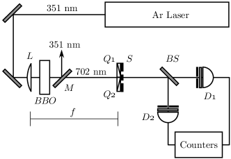
FIG. 1.: Experimental setup. $L$ is a lens of focal length $f=500$ mm, $BBO$ is a 2 mm-long $\beta$-BaB₂O₄ nonlinear crystal cut for collinear type II 351 nm$\rightarrow$702 nm down-conversion, $M$ is a u. v. high reflectance mirror, $Q_{1}$ and $Q_{2}$ are quarter-wave plates, $S$ is a double slit, $BS$ is a 50:50 beam splitter, $D_{1}$ and $D_{2}$ are avalanche photo-diodes working in photon counting mode.

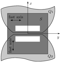
FIG. 2.: The birefringent double slit. $Q_{1}$ and $Q_{2}$ are quarter-wave plates aligned with orthogonal fast axes, and $S$ is a double slit with clear apertures of 0.20 mm$\times$5 mm separated by a 0.20 mm obstacle.

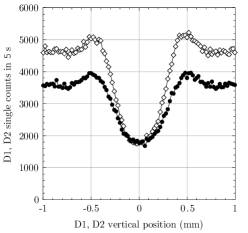
FIG. 3.: $D_{1}(\diamond)$ and $D_{2}(\bullet)$ single counts taken with a 0.20 mm diameter wire stretched horizontally in front of the beam splitter and the double slit removed. This measurement was taken in order to check the accuracy of detectors vertical positioning.

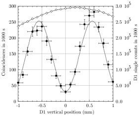
FIG. 4.: Single counts ($\diamond$) and coincidences ($\bullet$) taken with $D_{2}$ kept in $x_{2}=0$ and $D_{1}$ scanned vertically.

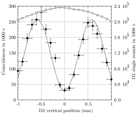
FIG. 5.: Single counts ($\circ$) and coincidences ($\bullet$) taken with $D_{1}$ kept in $x_{1}=0$ and $D_{2}$ scanned vertically.

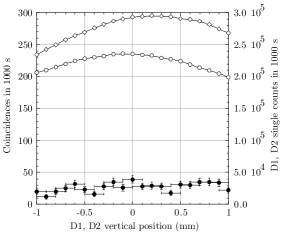
FIG. 6.: $D_{1}$ single counts ($\diamond$) , $D_{2}$ single counts $(\circ)$, and coincidences ($\bullet$) taken when both $D_{1}$ and $D_{2}$ were scanned vertically, keeping $x_{1}=x_{2}$.

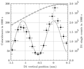
FIG. 7.: Single counts ($\diamond$) and coincidences ($\bullet$) taken with $D_{2}$ kept in $x_{2}=-0.55$ mm and $D_{1}$ scanned vertically.

REFERENCES

[1]
Electronic address: monken@fisica.ufmg.br
[2]
L. Mandel and E. Wolf, Optical Coherence and Quantum Optics
(Cambridge University Press, Cambridge, UK, 1995).
[3]
H. J. Carmichael and D. F. Walls, J. Phys. B 9, L43 (1976).
[4] H. J. Kimble and L. Mandel, Phys. Rev. A13, 2123
(1976).
[5] H. J. Kimble, M. Dagenais, and L. Mandel, Phys. Rev. Lett.39, 691 (1977).
[6] M. Le Berre-Rousseau, E. Ressayre, and A. Tallet,
Phys. Rev. Lett.43, 1314 (1979).
[7] D. N. Klyshko, Zh. Eksp. Teor. Phys. 83,
1313 (1982) [Sov. Phys. JETP 56, 753 (1982)].
[8] Z. Bialynicka-Birula, I. Bialynicki-Birula, and G.
M. Salamone, Phys. Rev. A43, 3696 (1991).
[9] M. I. Kolobov and I. V. Sokolov, Europhys. Lett.
15, 271 (1991).
[10] M. I. Kolobov, Rev. Mod. Phys. 71, 1539 (1999).
[11] C. H. Monken, P. H. Souto Ribeiro, and S. Pádua,
Phys. Rev. A57, 3123 (1998); E. J. S. Fonseca, C. H. Monken, S.
Pádua, and J. C. Machado da Silva, Phys. Rev. A61, 023801 (2000).
[12] W. A. T. Nogueira et al., to be published.
[13] A. V. Belinsky and D. N. Klyshko, Phys. Lett. A 166,
303 (1992).