Experimentally realizable characterizations of continuous variable Gaussian states

Abstract

Measures of entanglement, fidelity and purity are basic yardsticks in quantum information processing. We propose how to implement these measures using linear devices and homodyne detectors for continuous variable Gaussian states. In particular, the test of entanglement becomes simple with some prior knowledge which is relevant to current experiments.

In the current development of quantum information processing, we have witnessed the importance of fidelity, entanglement and mixedness. In this paper, we propose feasible experimental schemes to measure these critical quantities for Gaussian continuous-variable systems. The proposed schemes require standard laboratory devices such as beam splitters and phase shifters and highly efficient homodyne detectors.

Entanglement has been mainly confined to theoretical discussions. Only very recently, Horodecki and Ekert Ekert investigated how to measure entanglement. Experimental studies on quantum correlation between two or more particles have been concentrated on tests of the Einstein-Podolsky-Rosen (EPR) paradox and Bell’s inequality because an experimental measure of entanglement was not so clear. The present paper proposes an experimental scheme to measure a degree of entanglement with some prior knowledge of the given state. There are some indirect ways to test entanglement, for example, by proving the fidelity higher than the classical limit in quantum teleportation Braunstein . However, this provides only a sufficient condition for entanglement. On top of that, how to measure the fidelity has not been thoroughly investigated. Here, we also propose an experiment to measure how close two states are.

Experiments on continuous-variable quantum information processing have been concentrated on Gaussian states Braunstein ; Walmsley ; Leuchs . This is because, due to extremely low efficiency and high dispersion in high-order nonlinear interaction, experiments have been based on linear transformation of fields initially in thermal equilibrium. In thermal equilibrium, a field is in a Gaussian thermal state Barnett97 and the linear transformation keeps the Gaussian nature Agarwal . The linear transformation of an input field to an output fields is due to a Hamiltonian composed of linear and/or quadratic bosonic operators $\hat{a}$ and $\hat{a}^{\dagger}$. Any linear transformation for two-mode fields can thus be represented by a product of single-mode squeezing, rotation and displacement operations and two-mode squeezing and beam-splitting operations Agarwal .

To measure how close a quantum state $\hat{\rho}_{1}$ is to a reference pure state $|\psi\rangle_{2}$, the fidelity is defined as ${\cal F}={}_{2}\langle|\hat{\rho}_{1}|\psi\rangle_{2}$. The fidelity is important, for example, to find how successfully a state is reproduced after a set of local quantum operations and classical communications such as a teleportation process. However this theoretical concept has not been thoroughly investigated by experiment. We propose a feasible experimental scheme to realize the measurement of the fidelity.

It is convenient to work with the Weyl characteristic function defined as $C_{i}({\bf x})=\mbox{Tr}\hat{\rho}_{i}\hat{D}_{i}({\bf x})$. Here, the displacement operator is defined as $\hat{D}_{i}({\bf x})=\exp(i\hat{{\bf x}}_{i}{\bf x}^{T})$, where the operator vector $\hat{{\bf x}}_{i}=(\hat{q}_{i},\hat{p}_{i})$ with quadrature operators $\hat{q}_{i}=(\hat{a}_{i}+\hat{a}^{\dagger}_{i})$ and $\hat{p}_{i}=i(\hat{a}^{\dagger}_{i}-\hat{a}_{i})$ and the coordinate vector ${\bf x}=(p,-q)$. The fidelity $\cal F$ is equivalent to the overlap between the characteristic functions:

$${\cal F}=\frac{1}{\pi}\int d{\bf x}C_{1}({\bf x})C_{2}(-{\bf x}).$$ (1)

Throughout the paper, matrices are represented in bold face and operators with hats. In order to measure the fidelity of two fields, they are mixed at a beam splitter whose action is described by $\hat{B}_{12}=\exp[\theta(\hat{a}_{1}^{\dagger}\hat{a}_{2}-\hat{a}_{1}\hat{a}^{\dagger}_{2})]$, where the reflectivity $r$ and transitivity $t$ of the beam splitter are determined by $\theta$: $r=\sin\theta$ and $t=\cos\theta$. The characteristic function for an output field is

$$C_{out}({\bf x})=\mbox{Tr}_{2}\hat{D}_{2}({\bf x})\mbox{Tr}_{1}\hat{B}_{12}\hat{\rho}_{1}\hat{\rho}_{2}=C_{1}(r{\bf x})C_{2}(t{\bf x}).$$ (2)

By Fourier transforming the characteristic function, the Wigner function, $W(\alpha)$, is obtained Barnett97 . Thus we can easily see that the Wigner function of the output field at the origin ($\alpha=0$) of phase space is directly related to the fidelity:

$${\cal F}=\frac{1}{2\pi}\int d{\bf x}C_{out}({\bf x})=2\pi W(0)$$ (3)

when $r=-t=1/\sqrt{2}$. We have found that, after mixing the two fields at a 50:50 beam splitter, we measure the Wigner function at the origin of the phase space for one of the output fields, to find how close the two input fields are. The Wigner function of a given field can be measured using optical tomography Vogel , which requires some numerical processes on experimental data. However, if both the input fields are Gaussian, as the output field is also Gaussian, $W(0)$ is easily measured using a highly efficient homodyne detector.

The characteristic function of any single-mode Gaussian field is written as

$$C({\bf x})=\exp(-\frac{1}{2}{\bf x}{\bf V}_{s}{\bf x}^{T}+i{\bf d}{\bf x}^{T})$$ (4)

where ${\bf V}_{s}$ is the $2\times 2$ variance matrix defined as $(V_{s})_{ij}=\frac{1}{2}(\langle\{\hat{x}_{i},\hat{x}_{j}\}\rangle)-\langle\hat{x}_{i}\rangle\langle\hat{x}_{j}\rangle$ and ${\bf d}$ is the displacement vector $d_{i}=\langle\hat{x}_{i}\rangle$. The quadrature variables are measured by a balanced homodyne detector Yuen , which is a well-known device to detect phase-dependent properties of an optical field. The operational representation of the balanced homodyne detector is $\hat{O}_{HD}=\hat{q}\cos\chi+i\hat{p}\sin\chi$, where $\chi$ depends on the local-oscillator phase. The value $W(0)$ of the Wigner function is rotationally invariant so the numerical process becomes simpler as we rotate the output field to diagonalize the variance matrix ${\bf V}_{s}$. This can be done by placing an optical phase shifter before the homodyne detector. When the variance matrix is diagonalized the uncertainty $\Delta q\Delta p$ is minimized and the fidelity (3) is

$${\cal F}=\frac{1}{\Delta q\Delta p}\exp\left[-\frac{1}{2}\left(\frac{\langle\hat{q}\rangle^{2}}{\Delta q^{2}}+\frac{\langle\hat{p}\rangle^{2}}{\Delta p^{2}}\right)\right],$$ (5)

where $\langle\hat{p}\rangle$, $\langle\hat{q}\rangle$, $\langle\hat{p}^{2}\rangle$ and $\langle\hat{q}^{2}\rangle$ are measured by a homodyne detector. We have shown how the fidelity for two Gaussian fields is measured using a homodyne detector and a beam splitter. In relation to the two input fields, $\langle\hat{p}\rangle$ and $\langle\hat{q}\rangle$ are proportional to the displacement difference between them and $\Delta q\Delta p$ is the uncertainty over their averaged variance matrix. When the displacement difference for the two fields is zero, the fidelity is determined by their average uncertainty: ${\cal F}=1/\Delta p\Delta q$.

We have proposed an experimental scheme to measure the fidelity of two single-mode fields. We are now interested in how to measure the a degree of entanglement for a two-mode Gaussian field. In the discussion, we will be able to show how the entanglement measure is related to the mixedness of the system. The entanglement of a two-mode state does not change by displacement operation Kim02 so we write the general form of the characteristic function, $C({\bf x})$, for a two-mode Gaussian state without the linear displacement term in Eq. (4): $C({\bf x})=\exp(-{\bf x}{\bf V}{\bf x}^{T}/2)$, where ${\bf x}$ is now $(q_{1},p_{1},q_{2},p_{2})$ and ${\bf V}$ is a $4\times 4$ variance matrix for modes 1 and 2. The variance matrix can in fact be written using $2$ block matrices ${\bf L}_{1}$ and ${\bf L}_{2}$ for local quadrature variables and ${\bf C}$ and its transpose ${\bf C^{T}}$ representing inter-mode correlation,

$${\bf V}=\begin{pmatrix}{\bf L}_{1}&{\bf C}\\ {\bf C^{T}}&{\bf L}_{2}\end{pmatrix}.$$ (6)

What are the possible types of entangled continuous-variable states one can produce? We start with two independent fields of modes 1 and 2, which are in thermal equilibrium at temperatures $T_{1}$ and $T_{2}$, respectively. The variance matrix has only local elements, ${\bf L}_{1}=\tilde{n}_{1}\openone$ and ${\bf L}_{2}=\tilde{n}_{2}\openone$, where $\openone$ is the $2\times 2$ unit matrix and $\tilde{n}_{i}=1+2/[\exp(\hbar\omega/k_{B}T_{i})-1]$ with the Boltzmann constant $k_{B}$. The basic components of a linear transformation are single-mode squeezing, ${\bf S}_{i}(s)$, and rotation, ${\bf R}_{i}(\phi)$, and two-mode squeezing, ${\bf S}_{12}(s)$, and beam-splitting, ${\bf B}_{12}$, whose actions are described by their transformations of the variance matrix:

$${\bf S}_{i}(s)=\begin{pmatrix}\mbox{e}^{-s}&0\\ 0&\mbox{e}^{s}\end{pmatrix},~{}~{}{\bf R}_{i}(\phi)=\begin{pmatrix}\cos\phi&\sin\phi\\ -\sin\phi&\cos\phi\end{pmatrix},$$

$${\bf S}_{12}(s)=\begin{pmatrix}\cosh s\openone&\sinh s{\boldsymbol{\sigma}}_{z}\\ \sinh s{\boldsymbol{\sigma}}_{z}&\cosh s\openone\end{pmatrix},~{}{\bf B}_{12}=\begin{pmatrix}t\openone&-r\openone\\ r\openone&t\openone\end{pmatrix}$$ (7)

where ${\boldsymbol{\sigma}}_{z}$ is a Pauli spin matrix. Any combination, $\bf U$, of these matrices, transforms the variance matrix $\bf V$ into ${\bf U}^{T}{\bf V}{\bf U}$. Here, displacement has not been considered because it does not affect entanglement.

The degree, $s$, of squeezing normally determines the optimum entanglement for a given setup Kim02 . As squeezing is due to $\chi^{(2)}$-nonlinear interaction, the efficiency is relatively low and a combination of squeezers is not practical Loudon . Entangled states have been produced using two-mode squeezing ${\bf S}_{12}$ Braunstein ; Walmsley or the combination of ${\bf B}_{12}{\bf S}_{1}(r){\bf S}_{2}(-r)$ Leuchs . For these linear operations, the variance matrix is represented by diagonal ${\bf L}_{1}$, ${\bf L}_{2}$ and ${\bf C}$. In particular, if the two modes are initially in thermal equilibrium at the same temperature before a transformation, the local matrices ${\bf L}_{1}$ and ${\bf L}_{2}$ are identical, for which case we show that the degree of entanglement becomes simple and can be measured using joint homodyne detectors. If such a Gaussian field is decohered in two-mode thermal bath of which the two modes are in the same temperature, the decohered state is still represented by the same form of variance matrix LeeKim .

The inseparability of a continuous variable Gaussian state is determined by Peres-Horodecki condition Simon . A density operator $\hat{\rho}$ is entangled if and only if the partially transposed density operator $\hat{\rho}^{T_{2}}$ has any negative eigenvalues. In order to quantify entanglement, we define the degree of entanglement, ${\cal E}(\hat{\rho})$, as the absolute sum of the negative eigenvalues of the partially transposed density operator: ${\cal E}(\hat{\rho})=\mbox{Tr}|\hat{\rho}^{T_{2}}|-1$. This is an entanglement monotone Lee00 . In the following, we show how ${\cal E}(\hat{\rho})$ is related to homodyne measurements.

Lemma 1. – If the block matrices ${\bf L}_{1}={\bf L}_{2}$ and ${\bf C}$ are diagonal, i.e., the variance matrix of a Gaussian continuous-variable state has the following form:

$${\bf V}_{0}=\begin{pmatrix}n_{1}&0&c_{1}&0\\ 0&n_{2}&0&c_{2}\\ c_{1}&0&n_{1}&0\\ 0&c_{2}&0&n_{2}\end{pmatrix}$$ (8)

where $n_{1}$ or $n_{2}$ may be smaller than the vacuum limit 1. The degree of entanglement is given by

$${\cal E}(\hat{\rho})=\max\{0,(\delta_{1}\delta_{2})^{-1}-1\}$$ (9)

where $\delta_{i}=n_{i}-|c_{i}|$ for $i=1,2$.

We briefly sketch the proof. The main task is to calculate the trace of $|\hat{\rho}^{T_{2}}|$ which is the positive operator satisfying $|\hat{\rho}^{T_{2}}|^{2}=(\hat{\rho}^{T_{2}})^{2}$. In order to find the bound operator $|\hat{\rho}^{T_{2}}|$ and its trace, all operators are represented by their characteristic functions respectively, based on the one-to-one correspondence principle between a bound operator and its characteristic function Barnett97 . Then the operator equation, $|\hat{\rho}^{T_{2}}|^{2}=(\hat{\rho}^{T_{2}})^{2}$, is converted into an equation for their corresponding characteristic functions. The equality of the two Gaussian characteristic functions implies that their variance matrices and normalization values are the same. Let ${\bf V}_{p}$ and $N_{p}$ be the variance matrix and the normalization value for $|\hat{\rho}^{T_{2}}|$. The unit trace of $\hat{\rho}^{T_{2}}$ leads its normalization value to be unity: $\tilde{N}\equiv\mbox{Tr}\hat{\rho}^{T_{2}}=1$. Based on the observation that the transposition is momentum reversal, the variance matrix $\tilde{\bf V}_{0}$ of $\hat{\rho}^{T_{2}}$ is obtained from ${\bf V}_{0}$ with $\hat{p}_{2}\rightarrow-\hat{p}_{2}$. One thus has the two equations for ${\bf V}_{p}$ and $N_{p}$ as

$${\bf V}_{p}-{\boldsymbol{\Omega}}{\bf V}_{p}^{-1}{\boldsymbol{\Omega}}^{T}=\tilde{\bf V}_{0}-{\boldsymbol{\Omega}}\tilde{\bf V}_{0}^{-1}{\boldsymbol{\Omega}}^{T}$$ (10)

$$N_{p}=\sqrt{\frac{\mbox{det}{\bf V}_{p}}{\mbox{det}\tilde{\bf V_{0}}}}.$$ (11)

In addition, because $|\hat{\rho}^{T_{2}}|$ is positive, its variance matrix ${\bf V}_{p}$ satisfies the uncertainty principle Simon ,

$${\bf V}_{p}+i{\boldsymbol{\Omega}}\geq 0.$$ (12)

where ${\boldsymbol{\Omega}}=i{\boldsymbol{\sigma}}_{y}\otimes\openone$ with the Pauli spin matrix ${\boldsymbol{\sigma}_{y}}$. From the solution ${\bf V}_{p}$ satisfying both Eqs. (10) and (12), $N_{p}$ in Eq. (11) is obtained. Finally, the degree of entanglement ${\cal E}=N_{p}-1$ as $\mbox{Tr}|\hat{\rho}^{T_{2}}|=N_{p}$ and ${\cal E}$ is given in particular by Eq. (9) for ${\bf V}_{0}$. If and only if the partial transposed density operator is positive satisfying the uncertainty principle (12), ${\bf V}_{p}=\tilde{\bf V}_{0}$ and the state is separable with ${\cal E}=0$.

For the two-mode vacuum, $n_{1}=n_{2}=1$ and $c_{1}=c_{2}=0$ so that $(\delta_{i})_{0}=1$ where $({\boldsymbol{\cdot}})_{0}$ denotes the value for the vacuum. Recalling the definition of the variance matrix, $\delta_{1}=\frac{1}{2}(\langle q_{1}^{2}\rangle+\langle q_{2}^{2}\rangle-2|\langle q_{1}q_{2}\rangle|)$ and $\delta_{2}=\frac{1}{2}(\langle p_{1}^{2}\rangle+\langle p_{1}^{2}\rangle-2|\langle p_{1}p_{2}\rangle|)$, which can be measured by joint homodyne detectors for modes 1 and 2. According to Eq. (9) the state is separable with ${\cal E}=0$ when $\delta_{1}\delta_{2}\geq(\delta_{1}\delta_{2})_{0}$. Otherwise, the degree of entanglement is ${\cal E}(\hat{\rho})=(\delta_{1}\delta_{2})_{0}/(\delta_{1}\delta_{2})-1$. We have found that the entanglement of a Gaussian field in the form (8) can be tested by comparing the joint quadrature variance of the given field with that of the vacuum.

Let us consider the purity of a state. A degree of purity can be defined as $P=\mbox{Tr}\hat{\rho}^{2}=(1/2\pi)\int d{\bf x}C({\bf x})C(-{\bf x})$, where $C({\bf x})$ is the characteristic function of the given state. When $P=1$ the state is pure. The purity of a Gaussian state with its variance matrix ${\bf V}_{0}$ is easily calculated using the determinant of ${\bf V}_{0}$: $P=1/\sqrt{\det{\bf V}_{0}}$. We have already seen that the matrix elements of $V_{0}$ can be measured by homodyne detectors so the purity of the Gaussian state can be measured. To find the relation between the purity and entanglement, we define the mixedness $M$ of a system: $M=1-P$, which is zero when the system is pure and becomes unity when it is totally mixed. According to Lemma 1, a Gaussian state of the variance matrix ${\bf V}_{0}$ is separable when $\delta_{1}\delta_{2}-1\geq 0$. Multiplying a positive quantity $(n_{1}+|c_{1}|)(n_{2}+|c_{2}|)-1$ to the both sides of this inequality, we find the necessary and sufficient condition for separability: $M_{12}-M_{1}-M_{2}\geq 2|c_{1}c_{2}|$, where $M_{1}$ and $M_{2}$ are the mixedness of the field in mode 1 and 2 and $M_{12}$ is that of the whole field. For a pure two-mode state with $M_{12}=0$, the state is separable iff $M_{1}=0$ and $M_{2}=0$ with $|c_{1}c_{2}|=0$.

Figure 1: Configuration of the setup to test entanglement. The dotted devices measure off-diagonal terms of the local variance matrices ${\bf L_{1}}$ and ${\bf L_{2}}$. The boxed devices denoted by HD are homodyne detectors. The numbers refer to the modes.

So far we have assumed that the block matrices ${\bf L}_{1}$ and ${\bf L}_{2}$ and ${\bf C}$ are diagonal because this case is relevant to the current experimental conditions and the degree of entanglement becomes extremely simple. However, how do we make sure that there is vanishing off-diagonal matrix elements? Measuring the off-diagonal terms of local matrices is troublesome as it involves the joint measurement of two quadrature variables for a single mode. To measure the off-diagonal elements of ${\bf L}_{1}$ heterodyne , we put a 50:50 beam splitter which splits the field in mode 1 as schematically shown in Fig. 1. Using the beam splitter transformation in (7) with $r=t=1/\sqrt{2}$, we find that the field for three modes $1^{\prime},2$ and 3 is still Gaussian and its variance matrix is written as

$$\frac{1}{2}\begin{pmatrix}{\bf L_{1}}+\openone&\sqrt{2}{\bf C}&-{\bf L_{1}}+\openone\\ \sqrt{2}{\bf C^{T}}&{\bf L_{2}}&-\sqrt{2}{\bf C^{T}}\\ -{\bf L_{1}}+\openone&-\sqrt{2}{\bf C}&{\bf L_{1}}+\openone\end{pmatrix},$$ (13)

where the unit matrix $\openone$ is due to the vacuum injected into the unused port of the beam splitter. Now the off-diagonal elements of ${\bf L_{1}}$ can be measured by inter-mode correlation between modes $1^{\prime}$ and 3: The mean value of the joint measurement $\langle q_{1^{\prime}}p_{3}\rangle=-V_{12}/2$. Similarly other off-diagonal terms of the local variance matrices can be obtained.

In fact, we have shown how to find all the matrix elements of the variance matrix for a Gaussian field so that it is possible to test entanglement not only for the fields in the form (8) but also for any Gaussian field if the detection efficiency is unity. In this case we need to generalize the expression (9) for the degree of entanglement which is rather straightforward using the same argument to derive (9). An equivalent but alternative approach was suggested by Vidal and Werner Lee00 .

A homodyne detector is composed of two photodetectors. Inefficient photodetectors may miss photons to detect and reduces the quantum correlation between two modes. The detection efficiency thus determines the feasibility of the proposed schemes, in particular, to test entanglement of the field. If the efficiencies of the photodetectors are same, homodyne measurement by imperfect detectors is equivalent to homodyne measurement by perfect detectors following a beam splitter, one input port of which is fed by the field to be measured and the other by the vacuum Leonhardt94 . Here, we assume non-unit detection efficiency due only to missing photons to detect. The efficiency $\eta$ of the homodyne detector determines the transmission coefficient $\sqrt{\eta}$ of the beam splitter. In fact the fictitious beam splitter affects the testing field as though it is decohered in the vacuum reservoir. The detection efficiency, assumed the same for the both homodyne detectors, effectively changes the variance matrix from ${\bf V}$ to ${\bf V}^{\prime}=\eta{\bf V}+(1-\eta)\openone$. This is what is measured by imperfect homodyne detectors. If ${\bf V}$ is in the form ${\bf V}_{0}$, the variance matrix ${\bf V}_{0}^{\prime}$ takes the same form as ${\bf V}_{0}$ but with modified matrix elements $n^{\prime}_{i}=\eta n_{i}+(1-\eta)$ and $|c^{\prime}_{i}|=\eta|c_{i}|$ for each $i$.

Consider the effect of the detection efficiency on the inseparability of the testing fields. Substituting $n_{i}^{\prime}$ and $c_{i}^{\prime}$ into the separability condition, $\delta_{1}\delta_{2}\geq 1$, for inefficient detection, we find a state to be entangled when

$$(n^{\prime}-|c_{1}^{\prime}|)(n_{2}^{\prime}-|c_{2}^{\prime}|)=\eta^{2}(\delta_{1}\delta_{2}-\delta_{1}-\delta_{2}+1)$$

$$+\eta(\delta_{1}+\delta_{2}-2)+1<1.$$ (14)

Rearranging this equation, we can easily find that when the original testing field is characterized by $\delta_{1}+\delta_{2}<2$, it is always found to be entangled regardless of the detection efficiency unless the efficiency is zero. Fig. 2 presents the sets of Gaussian states on the space of $\delta_{1}$ and $\delta_{2}$ where separable states with $\delta_{1}\delta_{2}\geq 1$ are denoted by $S$ and entangled states with $\delta_{1}\delta_{2}<1$ by $E+E^{\prime}$. All entangled states in the region $E$ with the condition, $\delta_{1}+\delta_{2}<2$, will violate the inequality, $\delta_{1}\delta_{2}\geq 1$, unless the detection efficiency is zero while some entangled states in $E^{\prime}$ fail the test of entanglement.

Reid and Drummond derived the inequality for the quantum correlation between two mode fields along the line with the EPR argument Reid ; Leuchs . They introduced the uncertainty $V_{1}$ ($V_{2}$) between the observable $q_{1}$ ($p_{1}$) in one mode and $q_{1}^{\prime}$ ($p_{1}^{\prime}$) inferred from the observation of the other mode. Quantum correlation may lead the product of the uncertainties to be less than the vacuum limit, resulting in the inequality of $V_{1}V_{2}<1$. In our notation this inequality can be written as

$$\delta_{1}\delta_{2}<\frac{n_{1}n_{2}}{(n_{1}+|c_{1}|)(n_{2}+|c_{2}|)}.$$ (15)

Note that the right hand side of the inequality is always less than unity. Thus, the inequality (15) is sufficient to satisfy our inseparable condition (9) Ralph . However, the converse statement does not hold in general.

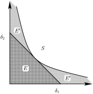
Figure 2: Gaussian states with the symmetric variance matrix ${\bf V}_{0}$ in Eq. (8). Separable states are denoted by $S$ and entangled states by $E$ and $E^{\prime}$ with the boundary of $\delta_{1}\delta_{2}=1$. Further the two regions $E$ and $E^{\prime}$ are separated by the line $\delta_{1}+\delta_{2}=2$. The entanglement imposed on a state of the region $E^{\prime}$ may fail the entanglement test due to inefficient detection. However, the entangled state of the region $E$ is always found to be entangled regardless of the detection efficiency.

We have proposed experimental schemes to measure the fidelity, the purity and the degree of entanglement of a given system with some prior knowledge. The scheme consists of beam splitters and balanced homodyne detectors which are well-established experimental tools to study quantum optics. When the detection efficiency is unity, the scheme can be extended to a general two-mode Gaussian state to test its entanglement.

We thank Prof. G. J. Milburn and Dr. M. Plenio for discussions and the UK EPSRC.

References

- (1) P. Horodecki and A. K. Ekert, quant-ph/0111064 (2001); A. G. White et al., Phys. Rev. A65, 012301 (2002).
- (2) A. Furusawa et al., Science 282, 706 (1998).
- (3) A. Kuzmich et al., Phys. Rev. Lett. 85, 1349 (2000).
- (4) Ch. Silberhorn et al., Phys. Rev. Lett. 86, 4267 (2001).
- (5) S. M. Barnett and P. M. Radmore, Methods in Theoretical Quantum Optics (Clarendon, Oxford, 1997).
- (6) H. Huang and G. S. Agarwal, Phys. Rev. A49, 52 (1994).
- (7) K. Vogel and H. Risken, Phys. Rev. A 40, R2847 (1989).
- (8) H. P. Yuen and H. J. Shapiro, IEEE Trans. Inf. Theory 24, 657 (1978).
- (9) M. S. Kim et al., Phys. Rev. A65, 032323 (2002).
- (10) R. Loudon and P. L. Knight, J. Mod. Opt. 34, 709 (1987).
- (11) J. Lee et al., Phys. Rev. A62, 032305 (2000).
- (12) R. Simon, Phys. Rev. Lett. 84, 2726 (2000).
- (13) J. Lee et al., J. Mod. Opt. 47, 2151 (2000); G. Vidal and R. F. Werner, Phys. Rev. A65, 032314 (2002).
- (14) This can also be measured using a heterodyne detector.
- (15) U. Leonhardt and H. Paul, Phys. Rev. Lett. 72, 4086 (1994).
- (16) M. D. Reid and P. D. Drummond, Phys. Rev. Lett. 60, 2731 (1988); M. D. Reid, Phys. Rev. A40, 913 (1989).
- (17) T. C. Ralph et al., Phys. Rev. Lett. 85, 2035 (2000); T. C. Ralph, quant-ph/0104108.