QUANTUM TUNNELING
In Memory of M. Marinov

Abstract

This article is a slightly expanded version of the talk I delivered at the Special Plenary Session of the 46-th Annual Meeting of the Israel Physical Society (Technion, Haifa, May 11, 2000) dedicated to Misha Marinov. In the first part I briefly discuss quantum tunneling, a topic which Misha cherished and to which he was repeatedly returning through his career. My task was to show that Misha’s work had been deeply woven in the fabrique of today’s theory. The second part is an attempt to highlight one of many facets of Misha’s human portrait. In the 1980’s, being a refusenik in Moscow, he volunteered to teach physics under unusual circumstances. I present recollections of people who were involved in this activity.

1 Introduction

I am honored to give this talk at the special session of the Israel Physical Society. A brief summary of Marinov’s life-long accomplishments in mathematical and high-energy physics was given by Professor Lipkin. My task was to choose one theme, from several which Misha considered to be central in his career, to show how deeply it is intertwined in the fabrique of today’s theory. I was asked to prepare a nontechnical presentation that would be understandable, at least, in part, to nonexperts.

The center of gravity of Marinov’s research interests rotated around advanced aspects of quantum mechanics, quasiclassical quantization and functional integration methods. For this event I have chosen the topic of quantum tunneling, which Misha cherished and to which he was repeatedly returning through his career, the last time in 1997. [1] The reader interested in a more technical discussion of Misha’s results on quantum tunneling is referred to Segev’s and Gurvitz’s articles in this Volume.[2, 3]

Apart from the direct involvement in the tunneling-related projects, this subject carries an imprint of other Marinov’s contributions – from dynamics of the Grassmannian variables [4] to the monopole studies in gauge theories.[5] I will explain this shortly. The second part of my talk is nonscientific. It is a sketch, an attempt to present one of many facets of Misha’s human portrait. In the 1980’s, being a refusenik in Moscow, he volunteered to teach physics under unusual circumstances. I conducted interviews with people who were involved in this activity.

2 What is quantum tunneling?

To demonstrate the essence of the phenomenon, let us consider a simple example – the $\alpha$ decay of heavy nuclei. For definiteness, one can keep in mind the decay

$$U_{92}^{238}\to Th_{90}^{234}+\alpha\,.$$

The energy of the emitted $\alpha$ particle in this decay is 4.7 MeV. The emitted $\alpha$ particle and the daughter $Th_{90}^{234}$ nucleus experience an interaction. At large distances this is the Coulomb repulsion

$$V_{\rm C}=\frac{Z_{1}Z_{2}e^{2}}{r}=\frac{2\times 90\times e^{2}}{r}=\frac{260}{r/\mbox{fermi}}\,\mbox{ MeV}\,.$$ (1)

The Coulomb potential is equal to 4.7 MeV at $r=55$ fermi. At such distances the nuclear force (which is attractive) is negligible since its range approximately coincides with the nucleus radius,

$$R_{n}\approx 1.2A^{1/3}=1.2\times(234)^{1/3}\approx 7.4\,\mbox{fermi}\,.$$ (2)

A sketch of the corresponding potential is shown in Fig. 1, where $V_{\rm C}^{*}\approx 35\,$MeV. At $r\!>\!R_{n}$ the potential is purely Coulombic, while at $r\!<\!R_{n}$ it is essentially determined by the nuclear interaction and is flat in a rough approximation. The energy of the $\alpha$ particle is denoted by $E_{1}$.

Figure 1: A sketch of the potential energy for $\alpha$ particle in the $\alpha$ decay of $U_{92}^{238}$.

At the initial moment of time the $\alpha$ particle is confined in the well at $r\!<\!R_{n}$. According to the laws of the classical mechanics it will stay there forever – the potential barrier at $R_{n}\!<\!r\!<\!R_{1}$ prevents the classical particle from the leakage in the domain to the right of $R_{1}$. Thus, classically $U_{92}^{238}$ is stable with respect to the $\alpha$ decay.

In actuality, the laws of quantum mechanics do allow the $\alpha$ particle to leak under the barrier. This is called “Quantum Tunneling.” The wave function of the $\alpha$ particle spreads under the barrier even if initially it was confined in the well to the left of $R_{n}$. If the barrier is high, as is the case in the problem at hand, the tunneling probability is exponentially small, and it can be calculated quasiclassically. The tunneling amplitude is proportional to 

$$A_{\rm tunneling}\propto\,\exp\left\{-\!\int_{R_{n}}^{R_{1}}\!\!\!\!\sqrt{2m(V-E_{1})}\,dr\right\}.$$ (3)

The integral in the exponent runs over the classically forbidden domain. The decay probability is given by $|A|^{2}$; it can be readily evaluated using the simple expression (3) which nicely explains the fact that the probability is extremely small, of order $10^{-37}$ in the problem at hand, and is extremely sensitive to the $\alpha$ particle energy. For all known $\alpha$-particle emitters, the value of $E_{1}$ varies from about 2 to 8 MeV. Thus, the value of the $\alpha$ particle energy varies only by a factor of 4, whereas the range of lifetimes (inverse probabilities) is from about $10^{11}$ years down to about $10^{-6}$ second, a factor of $10^{24}$.

The quantum tunneling as an explanation of the heavy nuclei decays was suggested by George Gamow [6] in 1928 and, somewhat later, (but independently) by Gurney and Condon.[7]

Figure 2: The double-well potential.

Quantum tunneling is at work in a much wider range of phenomena than the heavy nuclei decays just discussed. I chose this example for illustrative purposes since in these processes the consequences of the tunneling can be readily explained to nonexperts. The very same tunneling determines a global structure of the ground state in a wide variety of quantal and field-theoretical problems. For instance, in the text-book problem of the double-well potential (see Fig. 2), there is no instability. The tunneling from the left to the right well and vice versa manifests itself in that the ground state is unique (rather than doubly degenerate as would be the case in the classical theory). It is symmetric with respect to $x\!\to\!-\,x$, and there is an exponentially small energy splitting between the low-lying $P$-even and $P$-odd states. This splitting is determined by the very same expression (3) where one may put $E_{1}\!=\!0$, and the integral runs from $-\eta$ to $\eta$. It can be represented in an identical form as

$$A_{\rm tunneling}\propto\exp\,(-S_{0})\,,$$ (4)

where $S_{0}$ is the action on the classical trajectory $x(\tau)$ connecting the points $-\eta$ to $\eta$ in the distant past and distant future in the imaginary time. In the real time there are no classical trajectories connecting $-\,\eta$ and $\eta$, the domain between these two points is classically forbidden. The particle tunneling can be described as particle’s motion in the imaginary time, $t\!\to\!-\,i\tau$. Passing to the imaginary time, $t\!\to\!-\,i\tau$, we effectively change the sign of the potential, see Fig. 3. The double-well potential becomes two-hump. It is pretty obvious that in the two-hump potential there is a classical trajectory

$$m\,\ddot{x}=-\,\frac{dV}{dx}\,,\qquad V(x)=-\lambda\left(x^{2}\!\!-\eta^{2}\right)^{2}$$ (5)

interpolating between $-\,\eta$ and $\eta$. The minimal action is

$$S_{0}=\frac{m^{2}\omega^{3}}{12\lambda}\,.$$ (6)

Figure 3: The potential relevant to the imaginary time classical motion in the double-well problem.

This strategy is general in the problems of this type. The tunneling amplitude is determined (in the quasiclassical approximation) by the minimal action attained on the least-action trajectory interpolating through the classically forbidden domain in the imaginary time. In one-dimensional problems determination of such trajectories and calculation of the corresponding minimal action is a relatively trivial task. The task becomes exceedingly more complicated in multi-dimensional quantal problems and in field theory. Much of Marinov’s time and effort was invested in the theory of the multi-dimensional tunneling.

3 Multi-dimensional quantal problems

Now I would like to demonstrate, in some graphic examples, that 70 years after its inception the topic is alive and continues to attract theorists’ attention. The formulation of the problem to be discussed below is inspired by supersymmetry, although the corresponding dynamical systems need not be supersymmetric. Supersymmetry, by the way, was also very close to Marinov’s heart. The early work he did with Berezin [4] on the classical description of particles with spin in terms of the Grassmannian variables carries elements inherent to supersymmetry. Moreover, the last paper on which Misha worked being already terminally ill, was a historic essay on supersymmetry.[8]

In this section I will consider a class of quantal multi-dimensional problems. Assume that we have $n$ degrees of freedom, $X^{1},X^{2},...,X^{n}$, described by the Hamiltonian

$$H=\sum_{\ell=1}^{n}\,\frac{1}{2}\,\big{(}\dot{X^{\ell}}\big{)}^{2}\!+\,V\!\big{(}X^{\ell}\big{)}\,,$$ (7)

where the potential $V$ can be represented as

$$V=\frac{1}{2}\,\sum_{\ell=1}^{n}\left(\frac{\partial\,W\!({X})}{\partial X^{\ell}}\right)^{2},$$ (8)

$W$ is a function of all variables ${X}^{\ell}$, which I will call “superpotential”, bearing in mind its origin in supersymmetric theories. The mass $m$ is put $m\!=\!1$. This is done for simplicity, and is by no means necessary. In the given context the term superpotential is nothing but a convenient name for the function $W$.

Certainly, the potential (8) is very special. It has an interesting feature that at the extremal points of the superpotential,

$$\frac{\partial\,W\!({X})}{\partial X^{\ell}}=0\,,\qquad\ell=1,2,...,n\,,$$ (9)

the potential $V$ vanishes. Since the potential (8) is positive-definite these are the classical ground states of the system. Let us assume that Eq. (9) has more than one solution, and denote these solutions by $\xi_{a}\!\equiv\!\{\xi^{\ell}\}_{a}$ where the subscript labels distinct solutions,

$$\frac{\partial\,W\!({X}^{\ell})}{\partial X^{\ell}}=0\,,\quad\mbox{at}\quad X^{\ell}=\left(\xi^{\ell}\right)_{a}\,,\quad a=1,2,...$$ (10)

For simplicity I will assume that there are only two solutions, $\xi_{1}$ and $\xi_{2}$. This assumption does not lead to the loss of generality, it just makes the notation simpler. The barrier separating the points $\xi_{1}$ and $\xi_{2}$ is assumed to be high (see Fig. 4), so that the tunneling problem is solvable in the quasiclassical approximation.

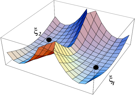
Figure 4: A profile of potential energy with two degenerate minima at $\xi_{1}$ and $\xi_{2}$. The barrier separating these two points is assumed to be high, so that tunneling can be described quasiclassically.

The tunneling amplitude from the first to the second classical minimum of the potential $V$ is given by Eq. (4), but finding the tunneling trajectory and the minimal action $S_{0}$ in case of a significant number of variables, $n\gg 1$, does not seem to be a trivial task, especially if the potential $V$ is contrived.

In fact, I will show momentarily that $S_{0}$ can be obtained [9] without solving the classical equations of motion for the trajectory,

$$S_{0}=\left|W(\xi_{1})-W(\xi_{2})\right|.$$ (11)

The classical equations in the imaginary time take the form

$$\ddot{X}^{\ell}=\frac{\partial\,V\!({X})}{\partial X^{\ell}}\,.$$ (12)

This is a second order differential equation. Consider, instead, the following first order differential equation

$${\dot{X}}^{\ell}=-\frac{\partial\,W\!({X})}{\partial X^{\ell}}\,.$$ (13)

If we manage to find a solution of this latter equation, it will be automatically the solution of Eq. (12). Indeed, differentiating both sides of Eq. (13) over $\tau$ one gets

$$\ddot{X}^{\ell}=-\sum_{j}\frac{\partial^{2}W}{\partial X^{\ell}\,\partial X^{j}}{\dot{X}}^{j}=\sum_{j}\frac{\partial^{2}W}{\partial X^{\ell}\,\partial X^{j}}\,\frac{\partial W}{\partial X^{j}}=\frac{\partial\,V\!(X)}{\partial X^{\ell}}\,.$$ (14)

(The inverse is not true).

Equation (13) has a very graphic physical interpretation – it describes the motion of a very viscous fluid (like honey) on the multi-dimensional profile given by $W(X_{\ell})$. The motion must originate in one extremal point of $W$ (which, obviously, must be a local maximum or a saddle point) and end up in the second extremal point (which must be a local minimum or a saddle point). The left-hand side is the velocity, there is no inertia; the right-hand side is the “force.” The velocity is proportional to the force. That’s how honey flows.

Although it may be difficult to find the flow trajectory analytically for contrived profiles, a rich mechanical intuition all of us have regarding this type of motion tells us immediately whether the solution exists or there is an obstruction, i.e. the honey flow from the summit is diverted away from the minimum, into an abyss. Once we see that the solution exists, we can get $S_{0}$ “for free”,

$$S_{0}=\frac{1}{2}\!\int\!\!d\tau\bigg{(}\!\sum_{\ell}\dot{X^{\ell}}\dot{X^{\ell}}+V(x)\!\bigg{)}\!\equiv\frac{1}{2}\!\int\!\!d\tau\!\left\{\!\bigg{(}\!\sum_{\ell}\!\dot{X^{\ell}}\!+\frac{\partial W}{\partial X^{\ell}}\bigg{)}^{2}\!\!\!-2\,\frac{dW}{d\tau}\!\right\}.$$ (15)

The expression in the parentheses on the right-hand side vanishes on the solution, while the second term, the full time derivative, yields Eq. (11).

It may happen that the flow equations (13) do not have a solution with the proper asymptotics – honey does not want to flow from the $a$-th to the $b$-th extremum of $W$. The second order equations (14) always do have a solution, however. From (15) we see that in this case $S_{0}>\!|W(\xi_{b})-W(\xi_{a})|\,,\,$ and

$$\exp\big{(}-\left|W(\xi_{b})-W(\xi_{a})\right|\big{)}$$ (16)

presents an upper bound on the tunneling amplitude.

The set-up described above (with the first order equations replacing the second order equations of motion) is called the Bogomol’nyi-Prasad-Sommerfield (BPS) saturation.[10, 11] BPS saturated objects are in the focus of today’s research in supersymmetric theories – from supersymmetric gluodynamics to string and brane theory, where the BPS saturation acquires a deep symmetry foundation. The BPS saturated objects preserve 1/2 or 1/4 of the original supersymmetry. The set-up was introduced by Bogomol’nyi in the pre-supersymmetry era. In 1975 Zhenya Bogomol’nyi was a Ph.D. student at ITEP, like myself. Immediately after the discovery of the ’t Hooft-Polyakov monopoles he started calculating their masses. The first calculation was numerical, a joint project with Misha Marinov.[5] In this work Bogomol’nyi and Marinov observed that the limit of the vanishing Higgs self-coupling was special; in this limit the monopole mass tended to $4\pi M_{W}\!/g^{2}$, with the coefficient exactly equal to 1. This observation served as a hint and an initial impetus for the subsequent work,[10] where the limit of the vanishing Higgs self-coupling was worked out analytically, and the monopole mass was reduced to a surface term, the magnetic charge.

4 Dynamics on manifolds

The above example describes dynamics generated by the potential $V\!(X)$ related to the superpotential $W\!(X)$ through Eq. (8). The space is flat, $X^{\ell}\!\in\!R_{n}$. In fact, one can readily generalize the problem to include the motion on nontrivial manifolds ${\cal T}$, endowed with the metric tensor $g_{ij}(X^{\ell})$,

$$L=\frac{1}{2}\,g_{ij}\dot{X}^{i}\dot{X}^{j}-\frac{1}{2}\,g^{ij}\frac{\partial W}{\partial X^{i}}\,\frac{\partial W}{\partial X^{j}}\,,$$ (17)

where the coordinates $X^{\ell}$ parametrize ${\cal T}$, and $W\!(X^{\ell})$ is a function on ${\cal T}$. As is evident from Eq. (17), the formula for the potential that replaces Eq. (8) is

$$V(X)=\frac{1}{2}\,g^{ij}\,\frac{\partial W}{\partial X^{i}}\frac{\partial W}{\partial X^{j}}\,.$$ (18)

I have already mentioned in the beginning of my talk that quantization on group manifolds (a particular class of nontrivial ${\cal T}$’s) was Misha’s perennial topic. Together with Terentev, he wrote a famous article on this subject.[12]

The BPS equations in this case take the form

$$\frac{dX^{i}}{d\tau}=-g^{ij}\frac{\partial W}{\partial X^{j}}\,,$$ (19)

with the boundary conditions that the trajectory starts at one minimum of the potential $V$ and ends at another (i.e. interpolates between two distinct extremal points of $W$). The solution of this equation interpolating between $\xi_{a}$ and $\xi_{b}$, if it exists, determines the minimal action and the tunneling amplitude (in the exponential approximation). As previously, the minimal action can be inferred without the knowledge of the explicit solution, and is given by the same formula, see Eq. (11). A remarkable feature is its metric-independence.

The existence/nonexistence of the solutions of Eqs. (19) depends on the global (topological) characteristics of the manifold ${\cal T}$ and the superpotential $W$. The corresponding theory – it goes under the name of the Morse theory – is a well-developed and quite beautiful branch of mathematics (see e.g. Refs.  [13] and  [14]). Unfortunately, I have no time to dwell on it, even briefly. The best I can do is to offer a simple illustration.

Let us assume that ${\cal T}$ is a two-dimensional sphere $S_{2}$, and the superpotential is such that it has two isolated extremal points, one at the north pole and another at the south (Fig. 5).

Figure 5: Tunneling trajectories for the particle on the sphere. The thick line is the flow line of the honey droplet from one extremal point of $W$ to another.

If one extremal point is the maximum of $W$, another one has to be the minimum. Alternatively, they can be saddle points. In both cases it is obvious that a droplet of honey, being placed in one extremal point, will find its way to another – the solution of the BPS equations always exists. In the first case (maximum at the north pole and minimum at the south), there exists a continuous family of solutions – the flow lines of the droplet can leave the pole along any meridian.

Now, one can start deforming ${\cal T}$ and $W$. For instance, one can squeeze the sphere of Fig. 5 transforming it into the surface of, say, a melon or a lemon, or another surface. As far as the existence of the BPS solution is concerned, nothing will change for small continuous deformations of ${\cal T}$ and $W$. The particular form of the solution will change, of course, but not the fact of its existence.

The solution connecting the north and south poles may disappear only if the deformations will be so strong that either topology of ${\cal T}$ changes or $W$ develops new extremal points which might trap the droplet on its way from one pole to another. If there are several extremal points, ${\cal T}$ splits into several domains – they are called the Morse cells. Each cell $M_{ab}$ presents a domain swept by the family of trajectories connecting $a$ and $b$,

$${\cal T}=\sum_{\rm pairs}M_{ab}\,.$$

5 Beyond physics

I would like to conclude my talk on a personal note. I first saw Misha Marinov when I came to ITEP around 1969 to pass my entrance examinations. The examination session was chaired by Professor V.B. Berestetskii. I do not remember exactly what topic was under discussion. I remember, however, that when a certain subtle point was raised, Berestetskii interrupted the session and said that at this point it would be appropriate to consult Okun. We went to his office, which was across the hall, and Marinov was there. Okun introduced us.

Since then we would occasionally bump into each other in the corridors of ITEP, or in the seminar hall. In 1979 Misha became a refusenik, a nonperson according to the Orwellian nomenclature. I remember that this news – that Marinov had applied for emigration to Israel – came when many of us were at the Odessa School of Physics organized by the Landau Institute. I heard Okun telling somebody that Marinov had left ITEP. In those days such a step actually meant “disappearance beyond the horizon”. In 1986, in the beginning of perestroika, when Marinovs finally got their exit visas to Israel, I came to their place to say farewell, since I was absolutely sure that I would never ever see any of them again (as were many other friends and colleagues who gathered in tiny Marinov’s apartment on Bolotnikovskaya street that night).

Well, life can be much richer than our imagination. It was not Marinov who was forced to give up his dream to live and die on the land of his ancestors, but, rather, the antihuman system which kept him hostage for years and to which he resisted, collapsed.

Many people in this audience knew Misha from the human side, as a person on whom one could always rely on a rainy day, always open to one’s needs and ready to help. I’d like to say a few words on that, dwelling on one of Misha’s activities which, regretfully, remains virtually unknown to public. In Marinov’s obituary in Physics Today (the September 2000 issue) it is mentioned that in the early 1980’s “… he volunteered to teach physics at the unofficial university organized by refuseniks to educate Jewish students who were barred by authorities from regular universities.”

In fact, Misha volunteered to teach at the so-called “Jewish People’s University” in Moscow which was organized in the late 1970’s by Bella Abramovna Subbotovskaya. At this time discrimination against Jews in the admission policies of the Soviet universities reached its peak. Sure enough, it was not the first peak, but it was especially strong. In fact, virtually all Departments of Mathematics in Soviet Union completely closed their doors to Jewish students. I do not know why, but (this is a well-known fact) the Soviet mathematical community, which gave to the world some of the most outstanding mathematicians, was also pathologically anti-Semitic. Such great mathematicians as Pontryagin and Vinogradov, who had enormous administrative powers in their hands, were ferocious anti-Semites. The tactics used for cutting off Jewish students were very simple. At the entrance examination special groups of “undesirable applicants” were organized. They were then offered killer problems which, as a rule, were at the level of international mathematical competitions; sometimes, they were flawed, or even completely wrong.

Bella Subbotovskaya’s idea was to launch something like unofficial extension classes, where children unfairly barred from the official universities could get food for their the hungry minds from the hands of the first-class mathematicians and physicists. It was supposed that the classes would take place on a regular basis through the entire school year, that they would be open to everybody (no registration or anything of this kind was required) and that the spectrum of courses offered would be broad and deep enough to provide a serious educational background in the exact sciences.

Andrei Zelevinsky (now at the North-Eastern University, Boston) recollects:

“Bella Abramovna was the main organizer […]. I didn’t know her very well: she was much older than me […]. It was she who brought Fuchs and me to teach there. I was truly impressed with her courage and quiet determination to run the whole thing. All the organizational work, from finding the places for our regular meetings to preparing sandwiches for participants was done by her and two other activists: Valery Senderov and […] Boris Kanevsky. Both as I understand, were active dissidents at the time. I think they made a deliberate effort to separate mathematics from politics, in order to protect us, professional research mathematicians.”

Another professor of this “university”, Dmitry Fuchs (now at UC, Davis), writes:

“We taught there major mathematical disciplines corresponding to the first two years of the Mekh-Mat curriculum: mathematical analysis, linear algebra and geometry, abstract algebra and so on. I taught there since 1980 through 1982, until Subbotovskaya’s sudden death in September or October of 1982 put an end to this enterprise. Bella Abramovna was tragically killed in a hit-and-run accident which was universally believed to be the act of KGB. This has never been officially confirmed though. At this time we did not use any particular name for our courses. In spirit, this was more a continuous seminar rather than a university. Among other teachers, I knew Andrei Zelevinsky, Boris Feigin, and Alexei Sossinski […]. The number of students varied between 60 and 20. The place of our meetings was not permanent: we met at an elementary school where Bella Abramovna worked as a teacher, at the Gubkin Institute for Petrol and Gas, at the Chemistry and Humanities Buildings of the Moscow State University, and so on. Anywhere, where we could get permission to occupy a large enough room…. I personally asked the Deputy Dean of the Chemistry Department for such a permission, and it was granted. All instructors prepared notes which were photocopied and distributed among the students. An article on our “school” was published by a Russian-Israeli newspaper some time ago. It was interesting but excessively emotional. Among other things, the authors had a tendency to exaggerate the Jewish nature of our “university.” It is certainly true that a substantial part of both, students and teachers, were ethnic Jews. This was the result of the well-known policy of the Mechmat admission committee, and the Soviet State at large, rather than the deliberate aim of the organizers. After all, we taught only exact sciences. No plans were made to teach Jewish culture, history, or language.”

Needless to say that all teachers were enthusiasts, and they received no reward other than the wonderful feeling that what they were doing was a good deed, a mitzva. Misha Marinov taught topics in physics.

Although the goals of this “university” were purely educational, the very fact of its existence was considered by the authorities as a political act of resistance. Any association with it was dangerous. The tragic fate of Bella Subbotovskaya remains uninvestigated so far. Perhaps, in the future her life will become a subject of a historical treatise, or a novel, who knows? Another activist who was mentioned above by Andrei Zelevinsky, Valery Senderov, was sentenced to 7 years in jail with the subsequent 5-year exile to Siberia on charges of anti-Soviet agitation and propaganda in 1983. One of the main pieces of incriminating evidence supporting the charges was his and Kanevsky’s essay Intellectual Genocide.[16] If one reads this essay now it is hard to understand how a person could be sent to prison for describing mathematical problems suggested to particular applicants at the entrance examinations at the Department of Mathematics of the Moscow University. Well, they say that everything goes in the struggle of classes. Why not mathematics?

But let me return to Misha and his generous contribution to this endeavor. A former student of Misha, Boris Shapiro recollects (his article [20] is published in this Volume):

“Soon after the beginning of the lectures on mathematics, Bella Abramovna announced that for all who desire to come, there would be a series of lectures by a famous physicist on quantum mechanics and field theory.[…] The very next Thursday, I think, in the tiny two-room apartment of Bella Abramovna on Nametkina Street, eight or nine people met, mainly second-year students […]. There appeared a tall, sinewy gray-haired man, with a slight lisp. The man was Misha Marinov, the name by which he introduced himself. By his appearance, Misha was close to forty-five years old; he had already been a refusenik for some time, and had seen a great deal. He had, until he applied for his exit visas, worked in ITEP and was personally acquainted with famous people. […] For me, he represented that heroic epoch when Jews were still accepted into the realm of physics and mathematics, where they uncovered so much. My impression was reinforced by occasional Misha’s stories of L.D. Landau, whose biography the younger generation was also eagerly reading. He spoke of his cooperation with F.A. Berezin, and it was then that I first heard of “supermanifold” […] On the other hand, once (during a tea break), he told us about a team of construction workers, shabashniks-refuseniks, to which he belonged, consisting entirely of Ph.D.  holders and professors. Those were dark times, and it was uncertain when and to where they would let him go. It was for this reason that Misha was very careful not to compromise the entire system of the “Jewish University” and other teachers, more or less well off and at that time far from any desire to immigrate. As they say, “some are no longer with us, and the others are far away…”.

The following quotation from Shapiro’s essay gives an idea of Misha’s choice of physics topics for teaching. It speaks also of his attitude, thoughtful and demanding. This was his usual attitude.

“Misha’s lectures were not simple. An understanding of mechanics, functional analysis, differential equations, differential geometry and the like was necessary. Despite this, I remember the ease and clarity with which he explained the fundamental ideas behind the difficult make-up of quantum mechanics. He pointed out the similarities and complexities of classical mechanics such that even I had the impression that I understood everything. I remember the interesting discussions on harmonic and anharmonic oscillators and the difficulties in the quantization of the latter. He even managed to discuss with the second-year students “supermathematics” on the basis of Grassmann algebra. […] He tried with all his strength to bring us to the level of current research, though this was not very realistic, meeting once a week with second-year students. In this way two intensive years went by, until in the spring of 1982 we were all stunned by the death of Bella Abramovna. Everyone went around very crushed, and the “Jewish University” soon fell apart.”

References

References

- [1] M. S. Marinov and B. Segev, “Quantum tunneling in the Wigner representation,” Phys. Rev. A 54, 4752 (1996) [quant-ph/9602017]; “Causality and time dependence in quantum tunneling,” Found. Phys. 27, 113 (1997); “Barrier penetration by wave packets and the ‘tunneling times,’ ” Phys. Rev. A 55, 3580 (1997) [quant-ph/9603018].
- [2] B. Segev, “Evolution kernels for phase-space distributions,” this Volume, p. 68.
- [3] S. A. Gurvitz, “Two-potential approach to multi-dimensional tunneling,” this Volume, p. 91.
- [4] F. A. Berezin and M. S. Marinov, “Particle spin dynamics as the Grassmann variant of classical mechanics,” Annals Phys. 104, 336 (1977).
- [5] E. B. Bogomolny and M. S. Marinov, “Calculation of the monopole mass in gauge theory,” Yad. Fiz. 23, 676 (1976).
- [6] G. A. Gamow, Zs. f. Phys. 51, 204 (1928); ibid 52, 510 (1928).
- [7] R. W. Gurney and E. U. Condon, Phys. Rev. 33, 127 (1929).
- [8] M. Marinov, “Revealing the path to the Superworld,” in The Many Faces of the Superworld, ed. M. Shifman (World Scientific, Singapore, 2000) p. 32.
- [9] B. Chibisov and M. Shifman, Phys. Rev. D 56, 7990 (1997); (E) D 58, 109901 (1998) [hep-th/9706141].
- [10] E. B. Bogomolny, Yad. Fiz. 24, 861 (1976) [Sov. J. Nucl. Phys. 24, 449 (1976)], reprinted in Solitons and Particles, eds. C. Rebbi and G. Soliani (World Scientific, Singapore, 1984) p. 389.
- [11] M. K. Prasad and C. M. Sommerfield, Phys. Rev. Lett. 35, 760 (1975), reprinted in Solitons and Particles, eds. C. Rebbi and G. Soliani (World Scientific, Singapore, 1984) p. 530.
- [12] M. S. Marinov and M. V. Terentev, “Dynamics on the group manifolds and path integral,” Fortsch. Phys. 27, 511 (1979).
- [13] J.F. Veverka, The Morse Theory and its Application to Solid State Physics (Queen’s University, Kingston, Ontario, 1966).
- [14] J. Milnor, Morse Theory (Princeton University Press, 1973).
- [15] B. Kanevsky, N. Meiman, V. Senderov and G. Freiman, Results of Admission of Graduates of Five Moscow Schools to the Department of Mechanics and Mathematics of Moscow University in 1981, Open Society Archives at Central European University, AC No 4696, (courtesy Ms. N. Zanegina).
- [16] B. Kanevsky and V. Senderov, Intellectual Genocide, Forschungsstelle OSTEUROPA of Bremen University, FSO, HA, F. 5/2 (courtesy Mr. G. Superfin).
- [17] G. Freiman, It Seems I am a Jew (Southern Illinois University Press, 1980).
- [18] A. Shen, “Entrance examination to the MekhMat,” The Mathematical Intelligencer, 16, No. 4, 6 (1994).
-
[19]
I. Vardi,
MekhMat entrance examination problems, see
http://www.ihes.fr/ĩlan (submitted for publication to the American Mathematical Society). I would like to thank Dr. Vardi for useful correspondence. - [20] B. Shapiro, “Underground ‘Jewish University,’ ” this Volume, p. 36.