Climbing Mount Scalable:
Physical-Resource Requirements
for a Scalable Quantum Computer

The primary resource for quantum computation is Hilbert-space dimension. Whereas Hilbert space itself is an abstract construction, the number of dimensions available to a system is a physical quantity that requires physical resources. Avoiding a demand for an exponential amount of these resources places a fundamental constraint on the systems that are suitable for scalable quantum computation. To be scalable, the effective number of degrees of freedom in the computer must grow nearly linearly with the number of qubits in an equivalent qubit-based quantum computer.

Key words: quantum information, quantum computation, entanglement, quantum mechanics, scalability

1 INTRODUCTION

Quantum computation is an alluring long-term goal for the emerging field of quantum information science [1]. In this paper we address the question of what physical resources are required for quantum computation and, in particular, how the required resources scale with problem size. We explicitly do not try to establish whether quantum computing is more powerful than classical computing, that being an unsolved problem in computational complexity theory. Rather we assume that quantum computing is more powerful than classical computing, and given this assumption, we ask how the physical resources required to take advantage of the power of quantum computing scale with problem size. By determining how to avoid a physical-resource demand that increases exponentially with problem size, we establish necessary conditions for a physical system to be a scalable quantum computer.

The initial step in a quantum computation [2] is to store classical information (the input) as some quantum state of the computer. The computer then runs through a carefully controlled sequence of unitary operations and/or measurements (the program). A program can be carried out wholly by reversible unitary operations [3] or wholly by irreversible quantum measurements [4–6]. Generally both will be used, especially in implementing quantum error correction [7–9] and fault-tolerant quantum computation [10–13]. At the completion of the computation, the answer (the output) is stored as classical information that can be read out with high probability by a measurement. The power of a quantum computer lies somewhere in the murky region between the classical input and the classical output—a region where classical, realistic descriptions fail.

Ask for the crucial property of that murky region, and you will get nearly as many answers as there are quantum information scientists: the superposition principle of quantum mechanics and associated quantum interference and quantum parallelism; quantum entanglement; the use of entangling unitary operations; the collapse of the wave function after measurement and associated information-disturbance trade-offs. All of these distinguish quantum systems from classical ones. How are we to decide which is the crucial quantum feature?

There are quantum-information-processing scenarios for which one or more of these features can be identified up front as a key resource not available in the comparable classical situation. Examples include quantum cryptography [14] and quantum communication complexity or distributed computing [15], where there are clearly identified, separate parties who can do things locally, but who interact with one another only through exchange of classical information. In quantum key distribution, for example, two parties seek to generate a secret key that can be used for secure communication. The presence of an eavesdropper is revealed by the disturbance produced when she obtains information about the key. In quantum communication complexity or distributed computing, separate parties try to perform some computational task through local operations and classical communication. Prior entanglement is a resource not available classically, which allows the parties to do things, such as teleportation, that can’t be done classically.

A quantum computer is not like these examples, however, because there are no clearly identified separate parties. Although it is natural to think in terms of a division of a quantum computer into parts that exchange quantum information, these parts are not like separate parties: they generally are not well separated, and they interact quantum mechanically with one another. Moreover, the division into subsystems is not unique [16], and there are proposals for quantum computing that have no natural division into parts at all [17–19].

Given that none of the quantum features listed above stands out as the source of a quantum computer’s power, we argue that the empowerment stems from the murky region itself: a quantum computer can escape the bounds of classical information processing because there is no efficient realistic description of what happens between the classical input and the classical output. We do not know how to characterize completely the circumstances for which there is no efficient classical description, since knowing this would be equivalent to knowing when a quantum computation is more powerful than a classical computation. If quantum computers are more powerful, however, their ability to access arbitrary states in Hilbert space leads to such situations.

It is difficult to pin down the source of a quantum computer’s power because arbitrary states can be accessed in very different physical systems—different hardware—using very different control techniques—different software, e.g., the use of reversible unitary operations vs. irreversible quantum measurements. Yet no matter how a quantum computation is packaged, we can identify one universal prerequisite: the computer must have a Hilbert space large enough to accommodate the computations. If the computer is to be a general-purpose computer, able in principle to solve problems of arbitrary size, it must have a Hilbert space whose dimension is capable in principle of growing exponentially with problem size. Hilbert space is essential for quantum computation, and the primary resource is Hilbert-space dimension.

Hilbert spaces of the same dimension are fungible. What can be done in one can be done in principle in any other of the same dimension: simply map one Hilbert space onto the other, including all the subsystems, operations, and measurements. Which Hilbert space is used to represent and process quantum information only becomes important when further physical considerations are introduced. What is important at the outset is that a system have “quantum information inside,” i.e., that there be information stored as arbitrary states in the system’s Hilbert space.

Though Hilbert spaces are fungible, the physical systems described by those Hilbert spaces are not, because we don’t live in Hilbert space, or as Asher Peres puts it [20], “Quantum phenomena do not occur in Hilbert space. They occur in a laboratory.” A Hilbert space gets its connection to the world we live in through the physical quantities—position, linear momentum, energy, angular momentum—of the system that is described by that Hilbert space. These physical quantities arise naturally from spacetime symmetries and the system Hamiltonian, and they are the physical resources that must be supplied to access various parts of the system Hilbert space. The crucial physical question for quantum computation is the following: how much of these resources is required to achieve a Hilbert-space dimension sufficient for a computation? This is the question we address in this paper.

Quantum mechanics—and its generalization to quantum fields—constrains our description of physical systems sufficiently that we can formulate the question of physical-resource demands in a general way. We find that to avoid supplying an amount of some physical resource that grows exponentially with problem size, the computer must be made up of parts—degrees of freedom in the simplest analysis, particles and field modes acting as effective degrees of freedom in the case of quantum fields—whose number grows nearly linearly with the number of qubits required in an equivalent quantum computer. This thus becomes a fundamental requirement for a system to be a scalable quantum computer [21].

This result will not be a surprise to researchers in quantum information science. Indeed, it is often assumed a priori that a quantum computer must be made up of interacting parts. Our analysis here provides a general justification for this requirement, based only on an examination of how Hilbert-space dimension is related to physical resources in different physical systems.

We emphasize that this requirement is an initial barrier that must be surmounted by proposals for scalable quantum computation, before such proposals confront the difficult tasks of initialization, control, protection from errors, and readout, to which we return at the end. Surmounting this barrier does not guarantee that a proposal can meet the further requirements; it is a necessary, but by no means sufficient requirement for a scalable quantum computer. An important point of this paper is that one can draw general conclusions about the physical systems that can be used for quantum computation just by considering whether the system can efficiently provide the primary resource of Hilbert-space dimension, without getting enmeshed in questions about the other necessary requirements for the operation of a quantum computer.

The remainder of the paper is organized as follows. In Sec. 2 we consider the physical resources required by a quantum computer that is built out of subsystems that are separate “degrees of freedom.” The conclusions drawn there form the core of our analysis, which we extend in Sec. 3 to systems that require a more general description in terms of quantum fields. In Sec. 4 we consider how our necessary condition for scalable physical resources is related to other requirements for quantum computation, including initialization, control, stability, and measurement. These requirements touch on some of the more difficult issues in trying to pinpoint the source of a quantum computer’s power, including the role of entanglement and the scalability of quantum computers that use highly mixed states. In Sec. 5, we summarize our conclusions.

2 DEGREES-OF-FREEDOM ANALYSIS OF RESOURCE
REQUIREMENTS

2.1 The Role of Planck’s Constant

Dimensionless quantities in physics are determined by writing the relevant physical quantities in terms of a relevant scale. For the dimension of a system’s Hilbert space, Planck’s constant $h$ sets the scale; the available number of Hilbert-space dimensions is determined by writing an appropriate combination of physical quantities, the action, in units of $h$.

The analysis of resource demands is particularly simple for systems of particles described by ordinary quantum mechanics, i.e., not requiring the more general description in terms of quantum fields. For these systems, the subsystems can be identified with the degrees of freedom of the particles. The quantum state of such a computer is described in a Hilbert space that is a tensor product of the Hilbert spaces of the degrees of freedom.

A degree of freedom corresponds to a pair of (generalized) canonical coördinates, position $q$ and momentum $p$. The physical resources are the ranges of positions and momenta, $\Delta q$ and $\Delta p$, used by the computation. The physically relevant measure of these resources is the corresponding phase-space area or action, $A=\Delta q\Delta p$. For a degree of freedom that is an intrinsic angular momentum $J$, we can use $\Delta q=2\pi$ and $\Delta p=\Delta J$, thus giving $A=2\pi\Delta J$. The connection to Hilbert space comes from the fact that a quantum state occupies an area in phase space given by Planck’s constant $h\,$; orthogonal states correspond roughly to nonoverlapping areas, each of area $h$ [22]. Thus the available dimension of the Hilbert space for a single degree of freedom is given approximately by $A/h$. The goal of scalability is to avoid having to supply an action resource $A$ for any degree of freedom that grows exponentially with problem size.

2.2 Degrees-of-Freedom Analysis

We measure the Hilbert-space dimension required for a quantum computation in qubit units: let the problem size for a computation be $n$, and let $N={\bf F}(n)$ be the number of qubits required for the computation, assuming an optimal qubit algorithm that requires only a polynomial number of qubits, an example being Shor’s factoring algorithm [2]. Here and throughout, bold type denotes a function that is bounded above by a polynomial. The Hilbert-space dimension needed for the computation is $2^{N}=2^{\mbox{\scriptsize\bf F}(n)}$. Using qubit units, we see that the Hilbert-space dimension grows exponentially with problem size. We assume that there is no more efficient algorithm in a Hilbert space with some other structure than the qubit tensor-product structure, this being part of our assumption that Hilbert spaces are fungible.

Suppose now that the $j$th degree of freedom supplies an action $A_{j}$. The Hilbert space of the entire system is a tensor product of the Hilbert spaces for the degrees of freedom, so the overall Hilbert space has dimension

$$2^{N}\sim{A_{1}\over h}\cdots{A_{T}\over h}={V\over h^{T}}\;,$$ (1)

where $V$ is the phase-space volume used by the computation. If $T$ grows more slowly than linearly with $N$ (within specific logarithmic corrections discussed below), at least one of the actions must grow exponentially with $N$, thus requiring an exponential amount of some physical resource. In contrast, if $T$ grows linearly with $N$, no degree of freedom has to supply an increasing amount of action, which makes the system a candidate for a scalable quantum computer.

It is useful to summarize this simple result, as it is the foundation for all our further conclusions. The physical resources are the quantities that label the axes of a (generalized) phase space that has two axes for each degree of freedom. The number of Hilbert-space dimensions available for a computation is proportional to the total phase-space volume. If the number of degrees of freedom grows linearly in $N$, the phase-space volume needed to accommodate the Hilbert-space dimension can be fitted into a hypercube in phase space without requiring an exponentially increasing contribution along any direction in phase space. In contrast, if the number of degrees of freedom grows more slowly than linearly in $N$ (within the logarithmic corrections), some phase-space direction must supply an exponentially increasing amount of the corresponding physical resource. This simple argument is depicted schematically in Fig. 1.

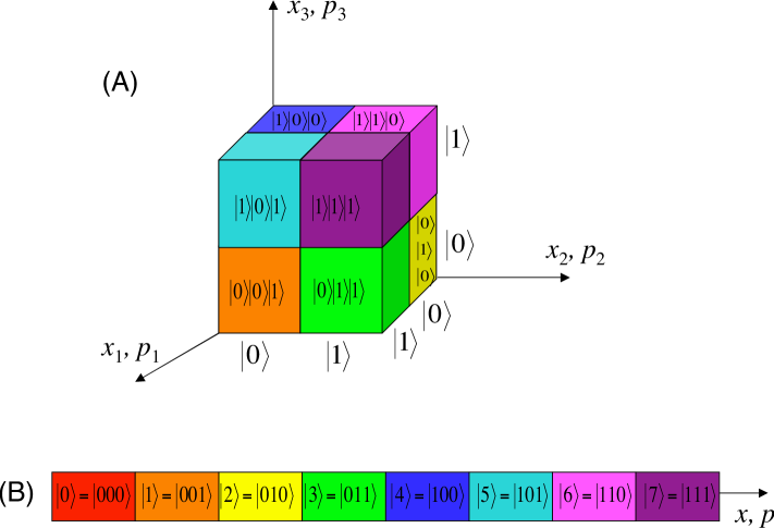
Figure 1: Using many degrees of freedom to save resources. Orthogonal basis states for an eight-dimensional Hilbert space depicted schematically as nonoverlapping phase-space cells in the phase space of three degrees of freedom (A), each of which uses an action $\sim 2h$, or in the phase space of a single degree of freedom (B). Phase space is pictured at half its actual dimension by letting the axes represent both the position and momentum coördinates for a degree of freedom; one can think of the axes as measuring the amount of action used by a degree of freedom. To accommodate the eight states, the single degree of freedom requires three times as much action as does each of the three degrees of freedom. If one adds degrees of freedom to (A), the phase-space volume—and hence the Hilbert-space dimension—doubles as each degree of freedom is added and thus grows exponentially with the number of degrees of freedom, whereas the physical resources grow linearly with the number of degrees of freedom and thus logarithmically with the Hilbert-space dimension. The result is a scalable resource requirement. In contrast, for the single degree of freedom in (B), the required resources grow linearly with phase-space volume and Hilbert-space dimension; to achieve the same Hilbert-space dimension as for the scalable case requires physical resources that are exponentially larger. As shown, the basis states for both situations can be labeled either by unary or binary numbers, this being an example of the fungibility of Hilbert spaces. The labeling, however, cannot alter the physics: the single degree of freedom is a physically unary realization of the Hilbert space, which uses exponential resources asymptotically, whereas the multiple degrees of freedom in (A) provide a physically binary realization of the same Hilbert space, which uses resources efficiently. The compact phase space achieved in (A) also aids in suppressing decoherence, as discussed in Sec. 4.3.

To formulate a more precise statement, we specialize to the case of $T$ identical degrees of freedom, each of which supplies an action $A$. In this situation, the total number of Hilbert-space dimensions satisfies $(A/h)^{T}\sim 2^{N}$, which gives

$$A/h\sim 2^{N/T}\;.$$ (2)

In order to avoid an exponential resource demand, $A/h$ must grow polynomially with $N$ [23], which means that the number of degrees of freedom increases as [24]

$$T\sim{N\over\log{\bf P}(N)}\;,$$ (3)

where ${\bf P}(N)$ is a function bounded above by a polynomial. We say that $T$ grows quasilinearly with $N$ and that the system is scalable, having a scalable tensor-product structure.

For comparison with our analysis of quantum fields, it is instructive to distinguish three cases:

1. $T$ grows more slowly than linearly with $N$. If $T$ grows quasilinearly, as in Eq. (3), then $A/h\sim{\bf P}(N)$, and the system is scalable. If $T$ grows more slowly than quasilinearly with $N$, $A/h$ grows exponentially with $N$, leading to an exponential demand for physical resources.

2. $T$ grows faster than linearly with $N$. Since $A/h$ goes to one as $N$ increases, the present analysis in terms of independent degrees of freedom breaks down and should be replaced by a counting of the excitations of a quantum field, which we give in Sec. 3.

3. $T=N/\log D$ grows strictly linearly with $N$. For $D<2$, the present analysis breaks down, and we again need the analysis of quantum fields to reach a sensible conclusion. For $D\geq 2$, each degree of freedom is a $D$-level system, i.e., a qudit instead of a qubit. Though this is a special case of quasilinear growth in which ${\bf P}(N)=D$, we separate it off for separate analysis. It is the most important scalable case because the action supplied by each system, $A/h\sim D$, is independent of problem size. Scaling is achieved simply by adding degrees of freedom, without having to change the Hilbert-space dimension supplied by each degree of freedom. We say that this kind of system is strictly scalable and has a strictly scalable tensor-product structure. Most quantum computing proposals are of this sort.

Had we focused on the total action resource,

$$TA/h\sim T2^{N/T}\;,$$ (4)

instead of on the action resource per degree of freedom, we would have reached the same conclusions regarding scaling. The total action resource is more akin to the resource quantities that arise in our analysis of quantum fields. For a scalable system, it grows as $TA/h\sim N{\bf P}(N)/\log{\bf P}(N)$; only for strictly scalable systems is the total action resource linear in $N$.

2.3 Quantum Computing in a Single Atom

An illuminating extreme example of the nonscalable systems in case 1 is the attempt to implement quantum computing in a single atom [17, 25, 26], fixed molecule [18], or large spin [19]. Advances in laser spectroscopy with ultrashort pulses have allowed researchers to manipulate and measure the electronic wave function in an atom [27] or both electronic and rotational/vibrational wave functions in a molecule [28] with exquisite precision. It is natural to wonder whether these tools for coherent control of quantum states can be applied to quantum computing.

For illustration, consider the simplest hypothetical model, quantum computing in a hydrogen atom. Characteristic atomic units of length, momentum, and energy are formed from the physically important constants: the electron charge and mass, $e$ and $m$, and the quantum of action, $\hbar$. If we ignore spin, Bohr’s formula for quantizing the action gives the familiar expressions for the energy, radius, and momentum of a stationary state with principle quantum number $n$,

$$E_{n}=-{1\over{2n^{2}}}\,{{e^{2}}\over{a_{0}}}\;,\quad r_{n}=n^{2}a_{0}\;,\quad p_{n}={1\over n}\,{\hbar\over{a_{0}}}\;,$$ (5)

where $a_{0}=\hbar^{2}/me^{2}$ is the Bohr radius. The dimension of the Hilbert space spanned by all bound states from the ground state up to a maximum principle quantum number $n$ is

$$\sum_{k=1}^{n}\sum_{l=0}^{k-1}(2l+1)\sim{1\over 3}n^{3}\sim\left({r_{n}p_{n}\over\hbar}\right)^{3}\;.$$ (6)

The final expression is of just the form we expect. Without spin the internal states of the hydrogen atom have three degrees of freedom, signaled by the 3 in the exponent and corresponding to the three coördinates of relative motion of the electron and proton. Each degree of freedom is allotted an action $A\sim r_{n}p_{n}$, which provides enough phase space for $\sim A/h$ orthogonal states in Hilbert space.

Demanding that the atomic Hilbert space have a dimension $2^{N}$ requires that the radial coördinate scale as $r_{n}\sim 2^{2N/3}a_{0}$. The exponential growth of this coördinate with problem size implies that quantum control in a single atom cannot be used for scalable quantum computation. For instance, to implement a quantum computation requiring $N=100$ qubits, the atomic radius must be $r_{n}\sim 10^{20}a_{0}=6\times 10^{6}\,$km, about 5 times the diameter of the Sun.

A single atom is an example of a “physically unary” quantum computer, having a limited natural tensor-product structure provided by the small number of physical degrees of freedom. Similar poor scaling will be seen in any implementation consisting of a single particle, a single atom, or a single molecule consisting of a fixed number of atoms. The fungibility of Hilbert spaces means that one can impose an artificial tensor-product structure on the Hilbert space of these systems, equivalent to that of qubits, but this does not obviate the need to provide the physical resources to generate orthogonal quantum states. Without a scalable tensor-product structure corresponding to a division into physical degrees of freedom, one or more of the physical coördinate axes must blow up exponentially with problem size, meaning that these systems are not suitable for scalable quantum computation.

This should be contrasted with quantum computing using multiple atoms, containing a physical tensor product structure, such as in an ion trap [29]. Quantum information is stored in two sublevels of each of the ion’s ground states and manipulated with a limited number of vibrational states. A Hilbert space of 100 qubits requires 100 ions in their ground states occupying 100 local positions. Neither the internal nor the external degrees of freedom of the atoms require physical resources that grow exponentially in order to accommodate a $2^{N}$-dimensional Hilbert space.

We now need to extend the lessons of this section to the more general case of quantum fields. In that context, the notion of degrees of freedom is generally not well defined, though in some circumstances it reëmerges as a useful concept. This more general analysis allows us analyze the cases that we were unable to treat properly above. Readers not interested in these details can skip the next section with little loss of continuity.

3 FOCK-SPACE ANALYSIS OF RESOURCE
REQUIREMENTS

3.1 Resources in Fock Space

We now consider a quantum field to be the basic physical system. The state of a single particle, i.e., a single quantum of excitation of the field, is described in a Hilbert space that is a tensor product of a $K$-dimensional Hilbert space for the particle’s external degrees of freedom (e.g., translational motion in three spatial dimensions) and a $D$-dimensional Hilbert space for the internal degrees of freedom (e.g., spin). The single-particle states represent different configurations of the quantum field, analogous to wave functions, and are often called field “modes.” The total number of modes is $M=KD$. Given the single particle space—“first quantization”—we can define the many-body system through the Fock-space construction—“second quantization.” Fock space is spanned by orthonormal Fock states, which are specified by giving the number of particles in each of the single-particle states.

The physical resources are the total number of particles, $L$, and the numbers of external and internal single-particle states, $K$ and $D$. We consider three kinds of systems: bose and fermi systems, and systems where each external state contains at most one particle. In the last of these, the particles are distinguished by the label for the external state and thus act like “distinguishable” particles. When $L=K$, each “distinguishable” particle has available $D$ internal states; hence this case reduces to $T=L=K$ particle degrees of freedom, each with $A/h=D$ levels, i.e., a quantum computer consisting of $L$ qudits.

For quantum fields, field and particle degrees of freedom are slippery concepts, which become rigorous only in special cases, such as the case of “distinguishable” particles just mentioned. In classical physics, particles and fields are both described by pairs of canonical coordinates, with the number of pairs determining the number of degrees of freedom. Thus a point particle moving in three dimensions has access to three degrees of freedom, and a vibrating string of limited bandwidth has access to a set of fundamental modes, each of which is a degree of freedom. The complementary particle and field aspects of a quantum field mean that physical degrees of freedom cannot generally be defined rigorously for quantum fields, since a rigorous definition requires that the overall Hilbert space be a tensor product of the Hilbert spaces for the individual degrees of freedom. The particle degrees of freedom of a quantum field come from a particle’s ability to occupy various single-particle states, but the restrictions set by particle indistinguishability mean that Fock space is not a tensor product of particle Hilbert spaces. The field degrees of freedom arise from the different numbers of particles that can occupy a single-particle state, or field mode. Although the entirety of Fock space is a tensor product of the field-mode Hilbert spaces, each spanned by particle-number states, the subspaces we are considering, which have no more than a fixed number of particles, are not. For example, for a bose field containing exactly $L$ particles, the states where any given mode contains all of the particles is in the subspace, but the tensor product of these states, where all modes contain $L$ particles, clearly is not.

The particle and field degrees of freedom of a quantum field can, nonetheless, be serviceable approximate concepts. It is useful to think in terms of particle degrees of freedom when the number of modes per particle, $M/L$, is large; we can then think of the $L$ particles as effective degrees of freedom. Likewise, field degrees of freedom are a useful approximate concept when the number of particles per mode, $L/M$, is large; in this case we can think of the $M$ modes as effective degrees of freedom. Outside these asymptotic regimes, particle and field aspects are both important, and the degrees of freedom are less useful concepts. Of course, for fermions, field degrees of freedom are never a useful concept, because the possible field excitations are so restricted by the Pauli exclusion principle.

For bosons, the physical resources can be interpreted in terms of a phase-space picture. The electromagnetic field provides a familiar example: the field modes give the possible states for a photon, and the population of the modes by photons describes the amplitudes of the electric and magnetic fields. The total number of modes, $M$, is proportional to the phase-space volume used by a single particle; it characterizes how ordinary space and particle momentum (wave number) and also internal states like photon polarization are used as resources. The number of particles, $L$, is proportional to the volume used in the phase space of the bose field; it characterizes how field strength is used as a resource. Because of the exclusion principle, only the particle aspect of this phase-space picture works for fermions, but that is sufficient for our considerations; since $L\leq M$, the number of modes is always the important resource for fermions.

Quantum entanglement is only defined for Hilbert spaces that have a rigorous tensor-product structure in terms of subsystems. Thus the structure of Fock space as a tensor product of field-mode Hilbert spaces has important implications for entanglement: entanglement among field modes is always well defined, but particle entanglement, along with particle degrees of freedom, can be defined rigorously only in special cases [19], an example being distinguishable particles with $L=K$. Note that when the field modes share just a single particle, mode entanglement is nothing more than the second-quantized version of a simple superposition state in the language of first quantization. These superposition states, e.g., the state of a single photon after it passes though a beam splitter, are indeed entangled states and can be used as an entanglement resource in protocols such as teleportation [30].

The Fock-space construction in hand, we proceed to counting Hilbert-space dimensions and analyzing resource requirements for the three kinds of systems. The counting is equivalent to calculating the entropy of a microcanonical ensemble in which all particles carry the same energy.

3.2 Scaling in Bose Systems

The dimension of the Hilbert space for $L$ bosons occupying $M$ modes is

$$\Omega_{B}={(M+L-1)!\over(M-1)!\,L!}\;.$$ (7)

This expression is invariant under the exchange $L\leftrightarrow M-1$; i.e., we can effectively exchange the roles of particles and modes in counting the number of orthogonal Fock states. For bosons it is often useful to consider the situation where the number of particles, instead of being fixed, can vary from zero to a maximum number $L_{\rm max}$. The corresponding Hilbert-space dimension can be obtained from $\Omega_{B}$ by increasing the mode number by 1, i.e., by imagining that there is an additional “phantom” mode that soaks up the extra particles:

$$\Omega^{\prime}_{B}={(M+L_{\rm max})!\over M!\,L_{\rm max}!}\;.$$ (8)

The particle-mode symmetry in this case is even simpler: $L_{\rm max}\leftrightarrow M$.

We consider whether this many-body system can support scalable quantum computation by examining the asymptotic behavior of $\Omega_{B}$ (or $\Omega^{\prime}_{B}$) in various cases.

1. $L$ fixed, $M$ grows: $2^{N}=\Omega_{B}\sim M^{L}/L!\,$. Particle degrees of freedom predominate. The system is not scalable because the number of modes must grow exponentially with $N$.

2. $M$ fixed, $L_{\rm max}$ grows: $2^{N}=\Omega^{\prime}_{B}\sim L_{\rm max}^{M}/M!\,$. Field degrees of freedom predominate. The system is not scalable because the number of particles must grow exponentially with $N$.

3. Both $L$ and $M$ grow:

   $$2^{N}=\Omega_{B}\sim\left(1+{L\over M}\right)^{M}\left(1+{M\over L}\right)^{L}\;.$$ (9)

   The first term represents field degrees of freedom, and the second term represents particle degrees of freedom. In this asymptotic regime the particle-mode symmetry reduces to $L\leftrightarrow M$. Again there are three cases.

   (i) $M$ grows faster than linearly with $L$: $N=\log\Omega_{B}\sim L\log(M/L)\Longrightarrow M\sim L2^{N/L}$ [this has the same form as the total action resource in Eq. (4)]. Particle degrees of freedom predominate, with $L$ being an effective number of degrees of freedom and $M$ being the resource that must be constrained. To be consistent with this case, $L$ must grow more slowly than linearly with $N$. As in our degrees-of-freedom analysis, if $L\sim N/\log{\bf P}(N)$ grows quasilinearly with $N$, the growth of $M\sim N{\bf P}(N)/\log{\bf P}(N)$ leads to a scalable resource requirement. If $L$ grows more slowly than quasilinearly with $N$, then $M$ grows exponentially with $N$, giving a nonscalable resource requirement.

   (ii) $L$ grows faster than linearly with $M$: $N=\log\Omega_{B}\sim M\log(L/M)\Longrightarrow L\sim M2^{N/M}$. Field degrees of freedom predominate, with $M$ being an effective number of degrees of freedom and $L$ being the resource that must be constrained. We reach the same conclusions as for (i), but with $L$ and $M$ reversed.

   (iii) $L=\mu M$, $\mu$ (constant) being the average number of particles per mode:

   $$2^{N}=\Omega_{B}\sim(1+\mu)^{M}(1+\mu^{-1})^{L}=2^{MS(\mu)}=2^{LS(1/\mu)}\;.$$ (10)

   Here $S(\mu)\equiv-\mu\log\mu+(1+\mu)\log(1+\mu)$ is the entropy (in bits) of a field mode containing on average $\mu$ quanta. The available Hilbert-space dimension is that of $M$ degrees of freedom, each with $2^{S(\mu)}$ levels, or $L$ degrees of freedom, each with $2^{S(1/\mu)}$ levels, in accordance with the particle-mode symmetry. This case is strictly scalable, as both $M$ and $L$ grow linearly with $N$. For $\mu\gg 1$, where field degrees of freedom predominate, the counting, $\Omega_{B}\sim\mu^{M}$, reduces to that of $M$ modes, each with $\mu$ levels. For $\mu\ll 1$, particle degrees of freedom predominate, and the counting, $\Omega_{B}=(\mu^{-1})^{L}$, reduces to that of $L$ particles, each with $\mu^{-1}$ levels; in this asymptotic regime, we recover the simple degrees-of-freedom analysis for the bose particles, each of which has access to a phase-space volume proportional to $\mu^{-1}$.

Examples of these different scenarios have been explored in the literature. Physically unary systems are a special instance of case 1 with a single particle ($L=1$) or of case 2 with a single mode ($M=1$). In a single-particle Fock space, we have $2^{N}=\Omega_{B}=M$, and there are two interesting possibilities: $D=1$, $K=M$ corresponds to single-photon optics [31, 32], whereas $K=1$, $D=M$ corresponds to an $M$-level system like an atom [17]. Both of these require an exponential number of modes and the associated physical resources. The case of many bodies occupying a single mode (case 2 with $M=1$) corresponds to quantum optics in a single-mode cavity; though this system has a large number of “nonclassical” states (e.g., squeezed states), the particle number must scale exponentially, $2^{N}=\Omega^{\prime}_{B}=L_{\rm max}+1$.

Closely related to unary systems with a single particle are implementations of quantum algorithms that use superposition and interference of classical linear waves. Classical linear optics (electromagnetic waves) provides an example that can be easily implemented in the laboratory. The wave amplitudes are described in a complex vector space, just like the Hilbert space of a quantum system, so it might appear that such classical-wave processors are candidate quantum computers. The problem is that they will always scale poorly when the necessary physical resources are taken into account. A classical wave is essentially a many-particle copy of a single-particle wave function. The linear-optics transformations of a classical wave are in one-to-one correspondence with the unitary transformations of the single particle wave function. The single photon has only three motional degrees of freedom and one polarization degree of freedom. Thus a classical-wave computation requires an exponential number of modes in the single-particle phase space [33], a demand inherited from a single-particle unary machine [34]. In addition, since the transformations required for a computation generally populate an exponential number of distinguishable modes, a classical-wave computation requires an additional exponential overhead in particle number (field strength) if all the populated modes are truly classical throughout the computation. This additional overhead can be avoided if one drops the demand for classical waves at all intermediate stages of the computation.

A compelling illustration of the physical-resource demands in classical linear-optical implementations was provided by Bhattacharya et al. [35] in a simulation of Grover’s algorithm for searching a database. The database entries were represented by the diffraction-limited transverse modes of a laser beam. Classical-wave interference leads to effective amplification of the sought-after mode, as Grover’s algorithm predicts. As the database grows with the corresponding number of qubits, however, the waist diameter of the beam must grow exponentially and would reach the size of the visible universe for $\sim 220$ qubits [36]. These same resource demands are seen in single-photon (unary) linear interferometers used to simulate quantum algorithms [31, 32].

The classical-wave example demonstrates that just having the necessary scalable Hilbert space is not sufficient to ensure scalable quantum computing. Classical waves are coherent states with a large mean particle number; the restriction to linear-optical transformations means that the field always stays within the coherent-state sector, never exploring the multitude of “nonclassical” many-body states. Whereas the Hilbert space of this many-boson, many-mode system can be made sufficiently large without exponential use of physical resources [case 3(iii)], the classical waves explore only a tiny portion of the available states. In doing so, classical-wave vector spaces end up demanding exponential resources to keep up with the quantum Hilbert space.

In contrast to classical waves, examples of bose systems that can take advantage of the favorable scaling of case 3(iii)—in particular, a proposal to use nonlinear optics as a source of interactions between pairs of photons [37]—were among the earliest proposals for quantum computation. More recently and more surprisingly, Knill, Laflamme, and Milburn [38] have demonstrated that just with linear optical unitary transformations—i.e., one-body transformations and no interactions between photons—one can implement scalable quantum computing, provided one has access to nonclassical field inputs and measurements of photon number, both of which take the field out of the coherent-state sector. In contrast, it has been shown [39, 40] that if one starts in a state with Gaussian statistics and has access only to manipulations within the so-called “Clifford semigroup” [40], which includes linear optics, squeezing, fast feedforward, and generalized measurements of canonical observables, but does not include photon counting, the result can be classically simulated and thus does not correspond to universal quantum computation. These examples demonstrate the subtlety of determining whether a given system has access to arbitrary states in Hilbert space.

3.3 Scaling in Fermi Systems

We now consider $L$ fermions distributed among $M$ modes ($L\leq M$). The number of distinguishable configurations gives rise to a Hilbert space of dimension

$$\Omega_{F}={M!\over L!\,(M-L)!}\;.$$ (11)

Fermi systems exhibit a particle-hole symmetry, $L\rightarrow M-L$. As with the bose case, we look at the asymptotic behavior to learn how the resource requirements scale.

1. $L$ fixed, $M$ grows: $2^{N}=\Omega_{F}\sim M^{L}/L!\,$. This is equivalent to case 1 for bosons, because the particles occupy the modes sparsely. We reach the same conclusion, i.e., this case is not scalable.

2. Both $L$ and $M$ grow:

   $$2^{N}=\Omega_{F}\sim\left({1\over 1-L/M}\right)^{M-L}\left({M\over L}\right)^{L}\;,\quad L\leq M\;.$$ (12)

   Now there are two subcases.

   (i) $M$ grows faster than linearly with $L$: $N=\log\Omega_{F}\sim L\log(M/L)$. This is identical to case 3(i) for bosons, since the particles are sparse, and we reach the same conclusions, i.e., scalability if $L$ grows quasilinearly with $N$, but not otherwise.

   (ii) $L=\mu M$, $\mu\leq 1$ (constant) being the average number of particles per mode and $1-\mu$ the average number of holes per mode:

   $$2^{N}=\Omega_{F}\sim(1-\mu)^{-(1-\mu)M}\mu^{-\mu M}=2^{MH(\mu)}\;.$$ (13)

   Here $H(\mu)\equiv-\mu\log\mu-(1-\mu)\log(1-\mu)\leq 1$ is the binary Shannon entropy corresponding to fraction $\mu$. The dimension of this Hilbert space is like that of $M$ degrees of freedom, each with $2^{H(\mu)}$ levels. The particle-hole symmetry becomes $\mu\leftrightarrow 1-\mu$. This system is strictly scalable since both $M$ and $L$ grow linearly with $N$. We recover an effective picture of particle degrees of freedom for $\mu\ll 1$, where $\Omega_{F}\sim(\mu^{-1})^{L}$, and of hole degrees of freedom for $1-\mu\ll 1$, where $\Omega_{F}\sim[(1-\mu)^{-1}]^{M-L}$. The largest Hilbert space arises for equal numbers of particles and holes, $\mu=1/2$, where $\Omega_{F}\sim 2^{M}=4^{L}$.

Examples of scalable fermi systems [case 2(ii)] have been investigated. Bravyi and Kitaev [41] showed that there is a universal gate set that consists of linear transformations together with a transformation coming from an interaction that is quartic in field amplitudes. In contrast to the bose case, the noninteracting fermi gas with measurements that count particles does not allow for universal quantum computation [42, 43]. Once again we see that access to a scalable Hilbert space is necessary, but not sufficient for performing quantum computation.

3.4 Scaling for “Distinguishable” Particles

When there is no more than one particle in each external state, the particles are effectively distinguishable. We assume $D\geq 2$ since $D=1$ reduces to the fermi case. The number of configurations is

$$\Omega_{D}={K!\over L!\,(K-L)!}D^{L}\;,\quad L\leq K.$$ (14)

As promised, we recover the qudit case when $L=K$, but we now have the freedom to explore the intermediate possibilities that arise when there are not enough particles to fill each of the external states, i.e., $1\leq L<K$. Here $K$ plays the role of the number of degrees of freedom in our simple degrees-of-freedom analysis, and $D$ plays the role of $A/h$. In contrast to the first-quantized picture, here $A/h=D$ gets raised to the power $L$, not $K$, when $L<K$, because not all the external states are occupied. This allows us to deal with the cases that we were unable to handle previously because we are now properly taking into account the resources required by unoccupied modes, i.e., vacuum.

We consider the number of internal states to be fixed in our analysis of the asymptotics, because the case where $D$ grows has already been dealt with in our simple degrees-of-freedom analysis. With this assumption, the asymptotic analysis goes as follows.

1. $L$ fixed, $K$ grows: $2^{N}=\Omega_{D}\sim(KD)^{L}/L!\,$. This is equivalent to case 1 for bosons and fermions, because the particles sparsely occupy the modes. The system is not scalable because the number of single-particle states must grow exponentially with $N$.

2. Both $L$ and $K$ grow:

   $$2^{N}=\Omega_{D}\sim\left({1\over 1-L/K}\right)^{K-L}\left({KD\over L}\right)^{L}\;,\quad L\leq K\;.$$ (15)

   Now there are two subcases.

   (i) $K$ grows faster than linearly with $L$: $N=\log\Omega_{D}\sim L\log(KD/L)$. This is a realization of case 2 in our simple degrees-of-freedom analysis, which we were unable to analyze because in that treatment we could not account for the resources required by unoccupied modes. Since the particles sparsely occupy the modes, this case is identical to case 3(i) for bosons and case 2(i) for fermions, i.e., scalable if $L$ grows quasilinearly with $N$, but not otherwise.

   (ii) $L=\mu K$, with $\mu\leq 1$ (constant):

   $$2^{N}=\Omega_{D}\sim(1-\mu)^{-(1-\mu)K}\mu^{-\mu K}D^{L}=2^{K[H(\mu)+\mu\log D]}\;.$$ (16)

   The system is strictly scalable with $K$ and $L$ linear in $N$: $L=\mu K=N/[H(\mu)/\mu+\log D]$. This provides the correct treatment of the remaining unanswered question in case 3 of the degrees-of-freedom analysis.

Though all these specific cases are tedious to analyze, there is a payoff, for they come together in a fundamental requirement for a many-body system to be a scalable quantum computer: scalability requires that the number of particles or the number of modes, whichever (or both) acts as the effective number of degrees of freedom, must grow quasilinearly with the equivalent number of qubits, $N$; if the effective number of degrees of freedom grows more slowly than quasilinearly in $N$, the complementary resource set demands an exponential supply of physical resources. This requirement is the analogue of our conclusion that a set of degrees of freedom must have a scalable tensor-product structure. The many-body analogue of strict scalability is that both $L$ and $M$ grow strictly linearly with $N$, this being the only case where all resources grow linearly with $N$.

4 OTHER REQUIREMENTS FOR A SCALABLE
QUANTUM COMPUTER

4.1 DiVincenzo Requirements

So far we have analyzed one necessary condition for a scalable quantum computer, based on the need to avoid an exponential demand for physical resources. We have been careful to emphasize that this requirement is necessary, but by no means sufficient. To see how the physical-resource requirement is related to other requirements for implementing a universal quantum computer, it is instructive to consider the list of five requirements laid down by DiVincenzo [3], which we have modified slightly for our purposes.

1. Scalability. A scalable physical system with well characterized parts, usually qubits.

2. Initialization. The ability to initialize the system in a simple fiducial state.

3. Control. The ability to control the state of the computer using sequences of elementary unitary operations chosen from a set of universal gates.

4. Stability. Long relevant decoherence times, much longer than the gate times, together with the ability to suppress decoherence through error correction and fault-tolerant computation.

5. Measurement. The ability to read out the state of the computer in a convenient product basis called the computational basis.

The first item in DiVincenzo’s list posits that a scalable quantum computer must be made up of parts with a strictly scalable tensor-product structure. Where does this requirement come from? Is it a prior requirement, independent of the other items in the list, or is it needed for initialization, control, stability, and efficient measurement? We argue here that a strictly scalable tensor-product structure is a prior requirement, above all others: in providing the primary resource of Hilbert-space dimension, a scalable system is necessary to avoid an exponential demand for physical resources, and a strictly scalable system is needed to constrain the demand for resources to grow as slowly as possible, i.e., linearly in the equivalent number of qubits.

DiVincenzo’s further requirements come into play once one has dealt with the resource issue. We suggest that a strictly scalable tensor-product structure makes it easier to achieve the control and stability requirements—so much easier, in fact, that one can regard a strictly scalable tensor-product structure as essential in practice for these two requirements. We turn now to a discussion of how the control and stability requirements are related to DiVincenzo’s first requirement, also touching on the question of quantum information processing using mixed states and the thorny question of the role of entanglement in quantum computing. We do not consider measurements issues explicitly, except as they arise in our discussion of the need for many measurements to read out the output of a mixed-state computer.

4.2 Control

Control of a quantum computation is accomplished via some set of elementary “universal” operations. In the quantum circuit model, these can be a finite set of one- and two-qubit quantum logic gates (unitary operators) [44] or an equivalent set of Hamiltonians that generate the one- and two-qubit dynamics [45, 46]. Alternatively, quantum algorithms can be implemented through a series of projective quantum measurements and classical control [4–6]. These schemes assume a tensor-product structure, usually a qubit decomposition. The qubit structure makes physical implementation of the elementary operations straightforward in principle; the coupling to the system needs to isolate either a single qubit or a pair of interacting qubits. Though many experimentalists will bridle at our use of “straightforward,” the control issues in systems without a tensor-product structure are far more serious, as noted by Ekert and Jozsa [47].

Consider, for example, quantum control of a unary system such as a single atom [17] or a large spin [19]. One control strategy is to map the one- and two-qubit gates onto the $2^{N}$ levels of the unary system. Even the simplest of the required gates, however, is difficult to implement in terms of operators that are physically relevant to the unary system. For instance, in a three-qubit system, the gate $\sigma_{x}^{(1)}\otimes I^{(2)}\otimes I^{(3)}$ generates a bit flip on the first qubit. Written in an 8-dimensional unary representation, this gate involves transitions between the $m$th level to the $(m\pm 4)$-th level, and all four transitions have the same strength. This involves coupling to the entire unary system, in contrast to the single-qubit coupling that is natural in a system made of qubits. The same problem arises for any mapping onto a “virtual subsystem” [16]. In practice, control of physically unary systems would be achieved by coupling directly to each level and by pairwise transitions between levels; since this requires access to a $\sim 2^{2N}$ control parameters, it is not scalable.

The relative ease with which a quantum system built out of subsystems can be controlled can be understood in terms of degrees of freedom. The physical quantities that quantify the resources for a degree of freedom provide the connection to the external world; precisely because they are physical observables, these physical quantities are available for building Hamiltonians that are controlled by an external classical apparatus. This allows the experimentalist to manipulate an exponential number of probability amplitudes with a polynomial number of gate operations.

4.3 Stability

A scalable tensor-product structure aids in suppressing decoherence and is probably essential for implementing quantum error correction and fault-tolerant quantum computation. The simplest analysis of the decoherence of quantum states that are widely separated in phase space gives a decoherence rate that is proportional to the square of the phase-space distance between the states [48, 49]. Our phase-space picture of the physical resources used by a quantum computation (see Fig. 1) shows that a qubit-based scalable quantum computer occupies a region of phase space that looks roughly like a $2N$-dimensional hypercube with side lengths independent of the number of qubits; the greatest distance between any two states in the accessible region of phase space is thus proportional to $\sqrt{2N}$. In contrast, in a unary system, where one degree of freedom bears the entire burden of the exponential increase of Hilbert-space dimension with problem size, the greatest distance between states grows at least as fast as $2^{N/2}$, i.e., exponentially with the equivalent number of qubits. This sharp difference suggests that a scalable tensor-product structure can play an important role in reducing decoherence. We emphasize that this argument is based on a very crude model of decoherence. Decoherence is not only highly system-specific, but difficult to characterize simply even for specific systems [50]. The significance of the argument is to suggest that a system whose accessible states are compactly arranged in phase space will not decohere faster than one whose states are distant in phase space and, under appropriate circumstances, will decohere much more slowly.

Once decoherence and noise in a physical system have been reduced below the error threshold for fault-tolerant quantum computation [10–13], quantum error correction [7–9] can be used to suppress errors sufficiently to perform arbitrarily long computations. Error-correction protocols cannot correct all errors. Instead they seek to correct the most probable errors, where what is most probable depends on the error mechanisms appropriate for a specific physical system; examples of such dominant errors include errors that act independently on individual qubits (though we refer to qubits, qudits could be used just as well) or errors that are correlated over many qubits. The most probable errors define an “error algebra” [9] of errors to be corrected. To detect and correct these errors, one encodes “logical qubits” into carefully chosen two-dimensional subspaces of several qubits. A good code is one such that the generators of the error algebra map the code subspace unitarily into mutually orthogonal subspaces. One is thus able to diagnose the error and correct it without destroying the encoded quantum information. We argue that these error-correction protocols require a scalable tensor product structure.

One set of errors that must be corrected consists of the inevitable imperfections in the quantum logic gates. Control of a set of qubits (or qudits) can be accomplished by a set of quantum logic gates whose number is polynomial in $N$. In contrast, as noted above, the natural couplings to a system that has no physical tensor-product structure are direct couplings to individual levels and pairwise transitions between levels. Arbitrary unitary operations can be built out of these elementary interactions, but since there are $\sim 2^{2N}$ elementary interactions, errors in them will lead to an exponentially large error algebra that contains essentially all errors, thus making error correction impossible.

Even if we had a more efficient scheme for constructing arbitrary unitaries, the known error-correction schemes still require a tensor-product structure. Error-correcting codes work by channeling the entropy introduced by noise and decoherence into ancillary subsystems (typically a number of qubits), which are reinitialized in a pure state for subsequent rounds of error correction. It is difficult to see how this could be managed in a system not made of parts that can be used as the ancillary subsystems. In particular, it is difficult to see how a virtual subsystem within a Hilbert space without a tensor-product structure could be reinitialized—or even how fresh virtual subsystems could be introduced.

4.4 Mixed-State Quantum Computing

Our analysis of physical-resource requirements assumed implicitly that the quantum system is described by a pure quantum state. Yet the system that has implemented the most sophisticated quantum-information-processing protocols is liquid-state nuclear magnetic resonance (NMR) [51–53], where the nuclear spins that act as qubits are described by a highly mixed state. A mixed-state quantum information processor can have a strictly scalable tensor-product structure, as do the nuclear-spin qubits of NMR, yet still require exponential resources because of the mixed nature of the quantum state. The problem is one of initialization. When the physical system is initialized in a mixed state, it has some probability to be in the desired initial pure state, along with probabilities to be in a variety of other undesired states; thus, at the end of the computation, the answer cannot be read out with high probability in a single measurement because the signal is buried in noise produced by the undesirable states. To extract the signal requires a number of measurements, made on copies of the physical system or on repetitions of the computation. Either of these amounts to an additional physical resource. The way this appears in mixed-state quantum information processors is that the signal is encoded in an expectation value that can be determined with good accuracy only from many measurements.

An example is provided by the present method for implementing quantum information processing in liquid-state NMR.  The processing elements are the active molecules in the liquid sample, each of which has $N$ active nuclear spins. The initialization procedure takes the $N$ nuclear spins from a state of thermal equilibrium, with polarization $\alpha\sim 2\times 10^{-5}$, to a so-called pseudopure state [51, 52], which has density operator $\rho=(1-\varepsilon)I/2^{N}+\varepsilon|\psi\rangle\langle\psi|$. This density operator is a mixture of the unpolarized, maximally mixed state of the spins, $I/2^{N}$, and the desired initial pure state, $|\psi\rangle\langle\psi|$. The mixing parameter $\varepsilon$ determines the size of the signal produced by the desired state; a consequence of pseudopure-state synthesis is that the mixing parameter decreases exponentially with the number of qubits, i.e., $\varepsilon=\alpha N/2^{N}$.

The exponential signal decrease is an in-principle problem for any information processing based on pseudopure-state synthesis [54]. To extract the signal from the random noise produced by the unpolarized piece of the density operator requires a number of copies or repetitions that scales as $1/\varepsilon^{2}=2^{2N}/\alpha^{2}N^{2}$, thus giving rise to an exponential resource demand. Even given the macroscopic number ($\sim 10^{20}$) of molecules in an NMR solution, each of which acts as an independent processor, liquid-state NMR is limited to about 20 qubits with the initial polarizations presently available.

Schulman and Vazirani [55] have outlined a method for distilling pure qubits from the weakly polarized nuclear spins in a liquid NMR sample. This method is algorithmic, using operations that can be implemented in NMR [56]. Though it is highly impractical, requiring $\sim 1/\alpha^{2}$ initial qubits for each distilled pure qubit, it does not make an exponential resource demand. From our perspective, however, this method is not an example of mixed-state quantum information processing. Rather it is a different initialization procedure, which cools a small subset of the qubits to zero temperature, using the remaining qubits as a heat reservoir, thus yielding an initial pure state to which our previous analysis applies.

We do not have a general analysis of the physical-resource demands posed by using mixed states for quantum information processing. We suspect, however, that computational protocols based on the use of highly mixed states suffer generally from a demand for an exponential number of repetitions or copies similar to that for pseudopure-state synthesis in liquid-state NMR. This hunch is supported by work [57] that suggests that supplementing a set of pure qubits with a supply of maximally mixed qubits provides almost no additional computational power beyond that in the pure qubits. These considerations make it unlikely that systems in highly mixed states can be scalable quantum computers, but this does not mean that they are equivalent to classical computers. They seem to lie somewhere between classical computers and full-scale quantum computers, since there are special problems [58, 59] for which no efficient classical algorithm is known, but which can be done efficiently using highly mixed states—without the need for an exponential number of copies or repetitions.

4.5 Entanglement

Entanglement is a distinctive feature of quantum mechanics. It is clearly a resource for such quantum information protocols as teleportation, yet its role in quantum computation remains unclear. Some claim it is the property that powers quantum computation [47, 60], while others downplay its significance [61, 62]. The situation has been clarified considerably by the recent work of Jozsa and Linden [63], who showed that for a qubit quantum computer—the extension to qudits is probably straightforward—entanglement among all the qubits is a prerequisite for an exponential speed-up over a classical computation. The Jozsa-Linden proof proceeds by showing that if entanglement extends only to some fixed number of qubits, independent of problem size, the computation can be simulated efficiently on a classical computer. Jozsa and Linden were careful to point out that although entanglement among all qubits is necessary for exponential speed-up, it is not sufficient: as shown by Gottesman and Knill [2], there are sequences of quantum gates that can be simulated efficiently even though they entangle all qubits.

The Jozsa-Linden argument assumes a strictly scalable tensor-product structure. The global entanglement that accompanies exponential speed-up is a consequence of assuming this tensor-product structure and an initial pure state. This does not necessarily imply that entanglement is the key resource for quantum computation. Consider a computation with an exponential speed-up on a qubit quantum computer. Mapped onto a unary machine, the same computation produces no entanglement. Whether run on the unary computer or the qubit computer, the computation accesses arbitrary states—i.e., arbitrary superpositions—in the computer’s Hilbert space and has no efficient description in the realistic language of classical computation. Hilbert spaces are fungible! Entanglement is not an inherent feature of quantum computation, but rather a result of running the computation on a quantum computer with a tensor-product structure; for such a computer, arbitrary superpositions lead to entanglement among all the parts, because the states without such entanglement occupy only a tiny corner of Hilbert space [47, 60]. On a physically unary computer, the same arbitrary superpositions have no entanglement.

We conclude that the global entanglement in a quantum computation is a consequence of the need to save resources, which is what dictates a strictly scalable tensor-product structure to start with. We suggest that entanglement, instead of being the power behind quantum computation, might be a measure of the computer’s ability to economize on physical resources. This surmise, based on our consideration of pure-state quantum computation, is supported by what is known about mixed-state quantum computation in liquid-state NMR.  The argument that entanglement follows from accessing arbitrary states in a system with a tensor-product structure doesn’t work for mixed states [63]. Indeed, with present polarizations, the states accessed in NMR are known to be unentangled up to about 13 qubits [64, 65] and, for bigger numbers of qubits, are likely to be far less entangled than in a corresponding pure-state quantum computer. This paucity of entanglement, we suggest, is a signal of the resource problem in NMR, i.e., the need, discussed above, for exponentially many molecules in NMR.

To investigate this idea further, one would like to quantify the amount of global entanglement produced in a quantum computation carried out in systems ranging from nonscalable to strictly scalable and including both pure-state and mixed-state realizations. This is a daunting task since there is presently no suitable measure of global entanglement in multipartite quantum systems, even for pure states. Indeed, multipartite entanglement cannot be summed up by any single measure and whether there is a measure or measures tied to the issue of scalability is far from clear.

5 Conclusion

Our contention in this paper is that the fundamental requirement for a scalable quantum computer is set by the need to economize on physical resources in providing the primary resource of Hilbert-space dimension. To avoid an exponential demand for physical resources, the number of degrees of freedom—or, for quantum fields, the number of particles or the number of field modes, depending on which (or both) acts as effective degrees of freedom—must grow quasilinearly with the equivalent number of qubits. These requirements mean that a scalable quantum computer must have a robust tensor-product structure. Systems without such a tensor-product structure are not suitable for scalable quantum computation.

Physical systems that don’t scale properly, such as liquid-state NMR, Rydberg atoms, or molecular magnets, are still worth studying for a variety of reasons. First and foremost, they embody fundamental physical questions that are worth investigating in their own right, regardless of their relevance to quantum information science. Second, they can be used to develop new technologies for control, readout, and error correction in quantum systems. These new technologies might have applications to quantum-information-processing jobs outside quantum computation, and they might be transferable to scalable quantum computers. Finally, the scalability criteria formulated in this paper are asymptotic requirements. They are useful for assessing the physical resources required for a general-purpose quantum computer to do problems of increasing size. Yet even for this purpose, they are imperfect tools, because no computer is expected to do problems of arbitrary size. Nonscalable systems might be able to provide sufficient Hilbert-space dimension for special-purpose quantum computations that need only a limited number of qubits, such as simulation of other quantum systems [66].

Hilbert space is essential for quantum computation. Yet it is an odd sort of thing to need. It is not a physical object, but rather a mathematical abstraction in which we describe physical objects [67, 68]. A Hilbert space gets a physical interpretation—a connection to the external world—only through the physical system that we describe in that Hilbert space. The connection is made through privileged observables—the generators of space-time symmetries, e.g., position, momentum, angular momentum, and energy—which determine a set of physical degrees of freedom for the system. This connection made, we can determine how the physical resources, measured in terms of phase-space actions constructed from the privileged observables, must grow in order to provide the Hilbert-space dimension needed for a quantum computation.

Our degrees-of-freedom analysis can be applied to the physical resources required by a classical computer. Generally the subsystems in a classical computer consist of many physical degrees of freedom. If each distinguishable configuration of a subsystem occupies a fixed phase-space volume $V_{0}$, then our analysis shows that the physical resources required by the classical computer grow exponentially unless the number of subsystems grows quasipolynomially with problem size. But the scale $V_{0}$ in the classical analysis is not fundamental, instead being set by noise and the resolution of measuring devices. This makes the classical analysis of resource requirements dependent on other features of a classical computer. The difference for a quantum computer is that Planck’s constant sets a fundamental scale, which makes the resource requirements presented here prerequisites for scalable quantum computation, prior to the other necessary requirements for a quantum computer’s operation.

Acknowledgments. This work was partly supported by the National Security Agency (NSA) and the Advanced Research and Development Activity (ARDA) under Army Research Office (ARO) Contract No. DAAD19-01-1-0648 and by the Office of Naval Research under Contract Nos. N00014-00-1-01578 and N00014-99-1-0247. This work grew in large part out of discussions at the Institute Theoretical Physics of the University of California, Santa Barbara, where the authors were in residence during the fall of 2001. The authors received support from the ITP’s National Science Foundation Contract No. PHY99-07949.

References

1. Quantum Information Science: An Emerging Field of Interdisciplinary Research and Education in Science and Engineering, Report of NSF Workshop, October 28–29, 1999, Arlington, VA, http://www.nsf.gov/cgi-bin/getpub?nsf00101.

2. M. A. Nielsen and I. L. Chuang, Quantum Computation and Quantum Information (Cambridge University Press, Cambridge, England, 2000).

3. D. P. DiVincenzo, Fortschr. Phys. 48, 771 (2000).

4. R. Raussendorf and H. J. Briegel, Phys. Rev. Lett. 86, 5188 (2001).

5. R Raussendorf and H. J. Briegel, “Computational model underlying the one-way quantum computer,” unpublished, arXiv.org e-print quant-ph/0108067.

6. M. A. Nielsen, “Universal quantum computation using only projective measurement, quantum memory, and the preparation of the $|0\rangle$ state,” unpublished, arXiv.org e-print quant-ph/0108020.

7. P. W. Shor, Phys. Rev. A 52, R2493 (1995).

8. A. Steane, Proc. R. Soc. London A 452, 2551 (1996).

9. E. Knill and R. Laflamme, Phys. Rev. A 55, 900 (1997).

10. D. Aharonov and M. Ben-Or, in Proceedings of the 29th Annual ACM Symposium on Theory of Computing (ACM Press, New York, 1997), p. 176; see also arXiv.org e-print quant-ph/9906129.

11. J. Preskill, Proc. R. Soc. London A 454, 385 (1998).

12. E. Knill, R. Laflamme, and W. H. Zurek, Science 279, 342 (1998).

13. E. Knill, R. Laflamme, and W. H. Zurek, Proc. R. Soc. London A 454, 365 (1998).

14. N. Gisin, G. Ribordy, W. Tittel, and H. Zbinden, Rev. Mod. Phys. 74, 145 (2002).

15. R. Cleve, in Quantum Computation and Quantum Information Theory, edited by C. Macchiavello, G. M. Palma, and A. Zeilinger (World Scientific, Singapore, 2000), p. 103.

16. P. Zanardi, Phys. Rev. Lett. 87, 077901 (2001).

17. J. Ahn, C. Weinacht, and P. H. Bucksbaum, Science 287, 463 (2000).

18. R. Zadoyan, D. Kohen, D. A. Lidar, and V. A. Apkarian, Chem. Phys. 266, 323 (2001); V. V. Lozovoy and M. Dantus, Chem. Phys. Lett. 351, 213 (2002). The authors of both these papers point out that the Hilbert space of a single molecule is not suitable for scalable quantum computation.

19. M. N. Leuenberger and D. Loss, Nature 410, 789 (2001).

20. A. Peres, Quantum Theory: Concepts and Methods (Kluwer, Dordrecht, 1993), p. 373.

21. Since in this paper we are interested in comparing how different systems use physical resources, we use the term quantum computer for any physical system that has the required Hilbert-space dimension, and we reserve the term scalable quantum computer for systems that can provide the required Hilbert-space dimension efficiently.

22. L.D. Landau and E.M. Lifshitz, Quantum Mechanics: Non-Relativistic Theory, 3rd Ed. (Oxford University Press, Oxford, 1998), p. 172.

23. We follow the computer-science convention of referring to any superpolynomial growth as exponential.

24. We use base-2 logarithms throughout.

25. D. A. Meyer, Science 289, 1431a (2000).

26. P. G. Kwiat and R. J. Hughes, Science 289, 1431a (2000).

27. M. W. Noel and C. R. Stroud, Jr., Phys. Rev. Lett. 77, 1913 (1996).

28. H. Rabitz, R. de Vivie-Riedle, M. Motzkus, and K. Kompa, Science 288, 824 (2000).

29. D. Kielpinski, C. Monroe, and D. J. Wineland, Nature 417, 709 (2002).

30. P.T. Cochrane and G. J. Milburn, Phys. Rev. A 64, 062312 (2001).

31. N. J. Cerf, C. Adami, and P. G. Kwiat, Phys. Rev. A 57, R1477 (1998).

32. P. G. Kwiat, J. R. Mitchell, P. D. D. Schwindt, and A. G. White, J. Mod. Opt. 47, 257 (2000).

33. J. F. Clauser and J. P. Dowling, Phys. Rev. A 53, 4587 (1996).

34. The exponential growth of physical resources required for readout in a classical wave computer and its relation to a unary quantum computer using a single photon has been noted by S. Wallentowitz, I. A. Walmsley, and J. H. Eberly, “How big is a quantum computer?” unpublished, arXiv.org e-print quant-ph/0009069.

35. N. Bhattacharya, H. B. van Linden van den Heuvell, and R. J. C. Spreeuw, Phys. Rev. Lett. 88, 137901 (2002).

36. Grover’s algorithm does not fit into our resource discussion because it does not provide an exponential speed-up relative to classical algorithms. Nonetheless, the experiment in Ref. 35 illustrates the resource demands that come with using classical waves.

37. G. J. Milburn, Phys. Rev. Lett. 62, 2124 (1989).

38. E. Knill, R. Laflamme, and G. J. Milburn, Nature 409, 46 (2001).

39. S. D. Bartlett, B. C. Sanders, S. L. Braunstein, and K. Nemoto, Phys. Rev. Lett. 88, 097904 (2002).

40. S. D. Bartlett and B. C. Sanders, “Efficient classical simulation of optical quantum circuits,” unpublished, arXiv.org e-print quant-ph/0204065.

41. S. B. Bravyi and A. Yu. Kitaev, “Fermionic quantum computation,” unpublished, arXiv.org e-print quant-ph/0003137.

42. B. M. Terhal and D. P. DiVincenzo, Phys. Rev. A 65, 032325 (2002).

43. E. Knill, “Fermionic linear optics and matchgates,” unpublished, arXiv.org e-print quant-ph/0108033.

44. A. Barenco, C. H. Bennett, R. Cleve, D. P. DiVincenzo, N. Margolus, P. Shor, T. Sleator, J. A. Smolin, and H. Weinfurter, Phys. Rev. A 52, 3457 (1995).

45. J. L. Dodd, M. A. Nielsen, M. J. Bremner, and R. T. Thew, Phys. Rev. A 65, 040301(R) (2002).

46. M. A. Nielsen, M. J. Bremner, J. L. Dodd, A. M. Childs, and C. M. Dawson, “Universal simulation of Hamiltonian dynamics for qudits,” unpublished, arXiv.org e-print quant-ph/0109064.

47. A. Ekert and R. Jozsa, Phil. Trans. R. Soc. London A 356, 1769 (1998).

48. W. H. Zurek, Phys. Today 44(10), 36 (1991).

49. D. Giulini, E. Joos, C. Kiefer, J. Kupsch, I.-O. Stamatescu, and H. D. Zeh, Decoherence and the Appearance of a Classical World in Quantum Theory (Springer, Berlin, 1996).

50. J. R. Anglin, J. P. Paz, and W. H. Zurek, Phys. Rev. A 55, 4041 (1997).

51. D. G. Cory et al., Fortschr. Phys. 48, 875 (2000).

52. J. A. Jones, Fortschr. Phys. 48, 909 (2000).

53. L. M. K. Vandersypen, M. Steffen, G. Breyta, C. S. Yannoni, M. H. Sherwood, and I. L. Chuang, Nature 414, 883 (2001).

54. W. S. Warren, Science 277, 1688 (1997).

55. L. J. Schulman and U. V. Vazirani, in Proceedings of the 31st Annual ACM Symposium on Theory of Computing (ACM Press, New York, 1999), p. 322; see also arXiv.org e-print quant-ph/9804060.

56. D. E. Chang, L. M. K. Vandersypen, and M. Steffen, Chem. Phys. Lett. 338, 337 (2001).

57. A. Ambainis, L. J. Schulman, and U. V. Vazirani, in Proceedings of the 32nd Annual ACM Symposium on Theory of Computing (ACM Press, New York, 2000), p. 697; see also arXiv.org e-print quant-ph/0003136.

58. E. Knill and R. Laflamme, Phys. Rev. Lett. 81, 5672 (1998).

59. R. Laflamme, D. G. Cory, C. Negrevergne, and L. Viola, Quant. Inf. Comp. 2, 166 (2002).

60. R. Jozsa, in The Geometric Universe: Science, Geometry, and the Work of Roger Penrose, edited by S. A. Huggett, L. J. Mason, K. P. Tod, S. T. Tsou, and N. M. J. Woodhouse (Oxford University Press, Oxford, England, 1998), p. 369.

61. S. Lloyd, Phys. Rev. A 61, 010301(R) (1999).

62. P. Knight, Science 287, 441 (2000).

63. R. Jozsa and N. Linden, “On the role of entanglement in quantum computational speed-up,” unpublished, arXiv.org e-print quant-ph/0201143.

64. S. L. Braunstein, C. M. Caves, R. Jozsa, N. Linden, S. Popescu, and R. Schack, Phys. Rev. Lett. 83, 1054 (1999).

65. N. C. Menicucci and C. M. Caves, Phys. Rev. Lett. 88, 167901 (2002).

66. S. Lloyd, Science 273, 1073 (1996).

67. C. M. Caves, C. A. Fuchs, and R. Schack, Phys. Rev. A 65, 022305 (2002).

68. C. A. Fuchs has promoted the notion that Hilbert-space dimension is a “characteristic property” of a quantum system, arXiv.org e-print quant-ph/0204146, or perhaps an “element of reality,” arXiv.org e-print quant-ph/0205039, which might be the realistic core of quantum theory.