Einstein-Podolsky-Rosen correlations of spin measurements in two moving inertial frames

Abstract

The formula for the correlation function of spin measurements of two particles in two moving inertial frames is derived within Lorentz-covariant quantum mechanics formulated in the absolute synchronization framework. These results are the first exact Einstein-Podolsky-Rosen correlation functions obtained for Lorentz-covariant quantum-mechanical systems in moving frames under physically acceptable conditions, i.e., taking into account the localization of the particles during the detection and using the spin operator with proper transformation properties under the action of the Lorentz group. Some special cases and approximations of the calculated correlation function are given. The resulting correlation function can be used as a basis for a proposal of a decisive experiment for a possible existence of a quantum-mechanical preferred frame.

I Introduction

Contemporary considerations of the Einstein-Podolsky-Rosen (EPR) Einstein et al. (1935); Bohm (1951) correlations are restricted mostly to observers staying in a fixed inertial frame of reference (for the theoretical prescriptions and experimental results see, e.g., Refs. Aspect et al. (1981, 1982a, 1982b); Bernstein et al. (1993); Bouwmeester et al. (1999); Pan et al. (2001); Stefanov et al. (2002); Tittel et al. (1998, 1999); Weihs et al. (1998); Zbinden et al. (2001)). This is motivated not only by the experimental requirement but, first of all, because of very serious difficulties connected with description of EPR-like experiments in frames in a relative motion. There are two reasons of the troubles with understanding and calculating the EPR correlation function in this case. The first one is related to the relativity of the notion of simultaneity for moving observers versus instantaneous state reduction. The second problem is related to the nonexistence of a covariant notion of localization in the relativistic quantum mechanics Bacry (1988). The latter deficiency is especially serious because every realistic measurement involves localization in the detector area.

Proposed solutions to these problems strongly depend on the adopted interpretation of quantum mechanics. From an orthodox point of view, attribution of physical meaning to the final probabilities only does not lead to a serious tension between quantum mechanics (QM) and special relativity, so they can “peacefully coexist” Aharonov and Albert (1981); Peres (1995, 2000a, 2000b).

The second line of understanding of QM lies in attributing a physical meaning to the physical state, its time evolution, localization, etc. From this point of view there are serious problems on the border between quantum mechanics and special relativity Bell (1981); Hardy (1992); Stapp (1977); Suarez ; Scarani and Gisin (2002). The most important ones are: lack of the manifest Lorentz covariance of quantum mechanics with finite degrees of freedom and the above mentioned nonexistence of a covariant notion of localization. Troubles with a sharp localization in the relativistic QM arise also if we restrict ourselves to a fixed inertial frame (cf. Hegerfeld theorem Hegerfeld (1998, 2001)).

Following Bell Bell (1981), a consistent formulation of quantum mechanics requires a preferred frame (PF) at the fundamental level (it is interesting that also Einstein and Dirac had admitted such a “nonmechanical” notion of a preferred frame Einstein (1922); Dirac (1951)). Bell gives the very clear point of view on to this question in Ref. Davies and Brown (1986).

A conceptual difficulty related to the notion of the PF lies in an apparent contradiction with the Lorentz symmetry. In Refs. Caban and Rembieliński (1999); Rembieliński (1980, 1997) it was shown that this is not the case: it is possible to arrange Lorentz group transformations in such a way that the Lorentz covariance survives while the relativity principle (democracy between inertial frames) is broken on the quantum level. Moreover, such an approach is consistent with all the classical phenomena. The physical meaning of the new form of the Lorentz group transformations lies in new, absolute synchronization scheme for clocks different from Einstein’s scheme Rembieliński (1980, 1997); Reichenbach (1969); Jammer (1979); Will (1992, 1993); Mansouri and Sexl (1977); Anderson et al. (1998). Both synchronizations, the new and the standard one, are physically inequivalent on the classical level only for velocities greater than the velocity of light. Furthermore, the causality notion, which is implied by the nonstandard absolute synchronization, is more general than the Einstein one and thus it is applicable to nonlocal phenomena. A Lorentz-covariant formulation of QM based on the above mentioned absolute synchronization scheme was given in Caban and Rembieliński (1999). In such a formalism it is possible to define the Lorentz covariant notion of localization and spin, i.e., covariant localized states and a covariant position operator as well as the spin operator transforming properly under the action of the Lorentz group. Note, that exactly these notions are relevant to a correct discussion of (non) locality in QM.

A serious candidate for a PF is the cosmic background radiation frame (CBRF); this choice is connected with possible dynamical (cosmological) distinguishing of a local privileged frame. Most recent EPR experiments performed in Geneva Scarani et al. (2000) have been analyzed according to PF hypothesis Caban and Rembieliński (1999) and give a lower bound for the speed of “quantum information” in CBRF at $2\times 10^{4}c$. Moreover some attention was also devoted to PF as a consequence of a possible breaking of the Lorentz invariance Coleman and Glashow (1999); Colladay and Kostelecký (1998) in high-energy processes.

Since the covariant spin operator also exists in the formulation of QM based on the absolute synchronization scheme Caban and Rembieliński (1999), therefore we can calculate precisely the EPR correlation function for any spin. To our knowledge, our results are the first exact EPR correlation functions obtained for Lorentz-covariant quantum-mechanical systems in moving frames under physically acceptable conditions (some attempts were given in interesting papers by Czachor Czachor (1997a, b); see however Ref. ). Because the resulting formula for the correlation function depends on the velocities of the preferred frame it can also help us to answer the old question concerning the existence of a PF by means of the quantum mechanical EPR experiment and possibly solve the dilemma posed by Bell.

II Preliminaries

II.1 Realizations of the Lorentz group in the absolute synchronization scheme

In this section we briefly describe main features of the absolute synchronization scheme mentioned above which is used in this work. The derivation of the presented results can be found in Refs. Caban and Rembieliński (1999); Rembieliński (1980, 1997). The main idea is based on a well-known fact that the definition of time coordinate depends on the procedure used to synchronize clocks Jammer (1979). If we restrict ourselves to the timelike or lightlike signal propagation, the choice of this procedure is a convention Jammer (1979); Mansouri and Sexl (1977); Reichenbach (1969); Will (1992, 1993); Anderson et al. (1998). Now, the form of Lorentz transformations depends on the synchronization scheme, and we can find a synchronization procedure which leads to the desired form of Lorentz transformation preserving instant time (i.e., $x^{0}=\mathrm{const}$) hyperplanes. To perform such a program one has to distinguish an inertial frame, called the preferred frame: Every absolute synchronization scheme (ASS) distinguishes formally such a priviledged inertial frame. We can go from one ASS to another by the action of the so-called synchronization group Caban and Rembieliński (1999); Rembieliński (1997). The classical relativity principle can be formulated in this language as the invariance of physical laws under the action of the synchronization group, or more simply, by the statement that each inertial frame can be chosen as the preferred frame, i.e., the choice of the preferred frame is physically irrelevant. The very serious advantage of ASS is the separation of the two fundamental notions of special relativity, namely, the relativity principle and the Lorentz covariance. In the absolute synchronization scheme, even in the case if the relativity principle is broken, the Lorentz symmetry survives.

Now, each inertial frame is determined by its four-velocity with respect to the preferred one. We shall denote the four-velocity of the preferred frame as seen by an observer at rest in an inertial frame by $u=(u^{0},\mathbf{u})$.

According to Refs. Rembieliński (1980, 1997) the transformation of the coordinates between inertial frames $O_{u}$ and $O_{u^{\prime}}$ takes the following form:

$$x^{\prime}(u^{\prime})=D(\Lambda,u)x(u),$$ (1a)

where $$\Lambda u O_{u} D(\Lambda,u) 4\times 4 \Lambda u$$ is an element of the Lorentz group, is the four-velocity of the preferred frame with respect to , and is a matrix depending on and . This equation must be accompanied by the transformation law for the four-velocity of a preferred frame, which [according to Eq. (1a)] takes the form

$$u^{\prime}=D(\Lambda,u)u.$$ (1b)

We point out that both Eqs. (1) are written for contravariant components of coordinate and four-velocity.

The explicit form of the matrix $D(\Lambda,u)$ is (see Refs. Caban and Rembieliński (1999); Rembieliński (1997)), for rotations

$$D(R,u)=\left(\begin{array}[]{c|c}1&0\\ \hline\cr 0&R\end{array}\right),$$ (2a)

where $$R\in\mathrm{SO}(3)$$ is a standard rotation matrix, and for boosts,

$$D(w,u)=\left(\begin{array}[]{c|c}(w^{0})^{-1}&0\\ \hline\cr-\mathbf{w}&I+\dfrac{\mathbf{w}\otimes\mathbf{w}^{T}}{1+\sqrt{1+|\mathbf{w}|^{2}}}-u^{0}\mathbf{w}\otimes\mathbf{u}^{T}\end{array}\right),$$ (2b)

where $w=(w^{0},\mathbf{w})$ denotes a four-velocity of the frame $O_{u^{\prime}}$ as seen by the observer in the frame $O_{u}$.

Hereafter we use the natural system of units with $c=\hbar=1$.

Transformations (1) leave the line element $ds^{2}=g_{\mu\nu}(u)dx^{\mu}\,dx^{\nu}$ invariant, where

$$[g_{\mu\nu}(u)]=\left(\begin{array}[]{c|c}1&u^{0}\mathbf{u}^{T}\\ \hline\cr u^{0}\mathbf{u}&-I+(u^{0})^{2}\mathbf{u}\otimes\mathbf{u}^{T}\end{array}\right).$$

Notice that $g(u)$ is constant (i.e., $x$ independent) in each inertial frame and is congruent to the Minkowskian metric $\eta=\mathrm{diag}(+,-,-,-)$. It is easy to check that the space element is Euclidean, i.e., $dl^{2}=d\mathbf{x}^{2}$.

The four-velocities $u$, $u^{\prime}$, and $w$ are related by

$$w^{0}=\frac{u^{0}}{{u^{\prime}}^{0}},\quad\mathbf{w}=\frac{(u^{0}+{u^{\prime}}^{0})(\mathbf{u}-\mathbf{u}^{\prime})}{1+u^{0}{u^{\prime}}^{0}(1+\mathbf{u}\cdot\mathbf{u}^{\prime})}.$$ (3)

The relation between coordinates in the standard and the absolute synchronization is given by

$$x^{0}_{E} =x^{0}+u^{0}\mathbf{u}\cdot\mathbf{x}, \mathbf{x}_{E} =\mathbf{x},$$ (4a)

$$u^{0}_{E} =(u^{0})^{-1}, \mathbf{u}_{E} =\mathbf{u},$$ (4b)

where the subscript $E$ indicates coordinates in the standard (Einstein’s) synchronization, while the coordinates in the absolute synchronization are written without any subscript. We see that only the time coordinate changes. Note also that in the same point of space we have $\Delta x^{0}_{E}=\Delta x^{0}$, so the time lapse is the same in both synchronizations. The coordinates $x_{E}$ in the Einstein’s synchronization transform according to the standard law, i.e., ${x^{\prime}}^{\mu}_{E}=\Lambda^{\mu}{}_{\nu}x^{\nu}_{E}$.

It is important to stress that the transformations (1) form a realization of the Lorentz group which transforms linearly space-time coordinates according to Eq. (1a) and simultaneously, nonlinearly transforms the PF four-velocity according to (1b). The round-trip velocity of light is invariant under Eqs. (1). In particular, the Reichenbach synchronization coefficient Reichenbach (1969); Jammer (1979) is given by $\epsilon(\mathbf{n},\mathbf{u})=(1-u^{0}\mathbf{n}\cdot\mathbf{u})/2$. Moreover, from Eqs. (4) we have the following relation between velocities in the absolute and the standard synchronizations:

$$\mathbf{v}=\frac{\mathbf{v}_{E}}{1-\dfrac{\mathbf{v}_{E}\cdot\mathbf{u}_{E}}{u^{0}_{E}}},$$ (5a)

$$\mathbf{v}_{E}=\frac{\mathbf{v}}{1+u^{0}\mathbf{v}\cdot\mathbf{u}}.$$ (5b)

Notice that for $|\mathbf{v}_{E}|>1$ the above formulas have singularities, i.e., if a superluminal propagation (possibly related to the nonlocality of the theory) takes place then both descriptions are no longer equivalent and consequently an ASS is physically distinguished in such a case even on the classical level Rembieliński (1997). It is remarkable that the velocity manifold of spacelike particles is a proper carrier space for the Lorentz group only in an ASS Rembieliński (1997).

We point out that the triangular form (2b) of a boost matrix implies that under Lorentz transformations the time coordinate is only rescaled by a positive factor, i.e., ${x^{\prime}}^{0}=x^{0}/w^{0}$, so the time ordering of events cannot be inverted by any Lorentz transformations between inertial frames, regardless of the space-time separation. This is important in the QM context because the transformations of time do not involve position operators.

II.2 Lorentz covariant quantum mechanics

The Lorentz-covariant QM was discussed in the framework of an absolute synchronization scheme in Ref. Caban and Rembieliński (1999). We associate with each inertial observer in $O_{u}$ a Hilbert space $\mathcal{H}_{u}$, so we have a bundle of Hilbert spaces rather than a single Hilbert space of states. It has been shown in Ref. Caban and Rembieliński (1999) that one can introduce Hermitian momentum and coordinate four-vector operators satisfying

$$[\hat{x}^{\mu}(u),\hat{p}_{\nu}(u)] =i\left(\frac{u_{\nu}\hat{p}^{\mu}(u)}{u_{\lambda}\hat{p}^{\lambda}(u)}-\delta^{\mu}_{\nu}\right),$$ (6a)

$${}[\hat{p}_{\mu}(u),\hat{p}_{\nu}(u)] =0,$$ (6b)

$$[\hat{x}^{\mu}(u),\hat{x}^{\nu}(u)] =0.$$ (6c)

We see that $\hat{x}^{0}$ commutes with all the observables. This allows us to interpret $\hat{x}^{0}$ as a parameter just like in the standard nonrelativistic quantum mechanics. Moreover, for $\hat{\vec{x}}$ Eq. (6a) is equivalent to $[\hat{x}^{i},\hat{p}_{k}]=i\delta^{i}_{k}$ and $[\hat{x}^{i},\hat{p}_{0}]=\hat{p}^{i}/\hat{p}^{0}$ (notice that the covariant components $u_{i}=0$ in each frame), i.e., it has the standard form. We stress that the commutation relations (6) are covariant in the absolute synchronization. In fact, we have the following transformation law for four-vector operators

$$U(\Lambda)\hat{x}^{\mu}(u)U^{{\dagger}}(\Lambda) =[D^{-1}(\Lambda,u)]^{\mu}{}_{\nu}\hat{x}^{\nu}(u^{\prime}),$$ (7a)

$$U(\Lambda)\hat{p}_{\mu}(u)U^{{\dagger}}(\Lambda) =[D^{T}(\Lambda,u)]_{\mu}{}^{\nu}\hat{p}_{\nu}(u^{\prime}),$$ (7b)

where $u^{\prime}=D(\Lambda,u)u$ and $D(\Lambda,u)$ is given by Eqs. (2). Using Eqs. (7) we can transform Eqs. (6) to another reference frame. We point out once again that under transformations (7a) for the time component $\hat{x}^{0}$ does not mix with spatial components $\hat{x}^{k}$ ($k=1,2,3$). One can also check that

$$[\hat{x}^{\mu}(u),\hat{p}^{2}(u)]=[\hat{p}_{\mu}(u),\hat{p}^{2}(u)]=0,$$ (8)

which means that a localized state has a definite mass. It is important to stress that the unitary map which connects one choice of ASS to another choice of ASS and preserves Eqs. (6) and (7) does not exist (this means that the synchronization group Caban and Rembieliński (1999); Rembieliński (1997) cannot be unitarily realized in this case). For this reason QM distinguishes an ASS, i.e., a particular preferred frame—the quantum preferred frame. In Ref. Rembieliński (1997) it was shown that the choice of the quantum preferred frame can be done by the spontaneous breaking of the synchronization group. As it was mentioned earlier, a natural candidate for quantum preferred frame is the CBRF .

Transformations of the Lorentz group induce an orbit in a bundle of Hilbert spaces $\mathcal{H}_{u}$. Unitary orbits are parameterized by mass and spin, similarly as for standard unitary representations of the Poincaré group.

An orbit induced by an action of the operator $U(\Lambda)$ in the bundle of Hilbert spaces under consideration is fixed by the following covariant conditions: (i) $k^{2}=m^{2}$, (ii) $\operatorname{sgn}(k^{0})$ is invariant; for physical representations $k^{0}>0$, $\operatorname{sgn}(k^{0})=1$. As a consequence there exists a positive defined Lorentz-invariant measure

$$d\mu(k,m)=d^{4}k\,\theta(k^{0})\delta(k^{2}-m^{2}).$$ (9)

Now, applying the Wigner method and using Eqs. (7) one can easily determine the action of the operator $U(\Lambda)$ on a basis of eigenvectors of the four-momentum operator Caban and Rembieliński (1999)

$$\hat{p}_{\mu}(u)|k,u,m;s,\sigma\rangle=k_{\mu}|k,u,m;s,\sigma\rangle.$$ (10)

We find

$$U(\Lambda)|k,u,m;s,\sigma\rangle=\mathcal{D}^{s}(R_{(\Lambda,u)})_{\lambda\sigma}|k^{\prime},u^{\prime},m;s,\lambda\rangle,$$ (11)

where the contravariant components $u^{\mu}$ and $k^{\mu}$ transform as follows

$$u^{\prime}=D(\Lambda,u)u=D(L_{u^{\prime}},\tilde{u})\tilde{u},$$ (12)

$$k^{\prime}=D(\Lambda,u)k,$$ (13)

while

$$\begin{split}R_{(\Lambda,u)}&=D(R_{(\Lambda,u)},\tilde{u})\\ &=D^{-1}(L_{u^{\prime}},\tilde{u})D(\Lambda,u)D(L_{u},\tilde{u})\in\mathrm{SO}(3).\end{split}$$ (14)

Here $\tilde{u}=(1,\mathbf{0})$, $u=D(L_{u},\tilde{u})\tilde{u}$ and $\mathcal{D}^{s}$ is the standard spin $s$ matrix representation of $\mathrm{SU}(2)$, $s=0,\frac{1}{2},1,\ldots$; $\sigma,\lambda=-s,-s+1,\ldots,s-1,s$. $R_{(\Lambda,u)}$ is a Wigner rotation belonging to the little group of a vector $\tilde{u}$. It should be noted that in this approach, contrary to the standard one, representations of the Poincaré group are induced from the little group of the vector $\tilde{u}$, and not $\tilde{k}=(m,0,0,0)$. Finally, the normalization condition for the basis vectors takes the form

$$\langle k,u,m;s,\lambda|k^{\prime},u,m;s^{\prime},\lambda^{\prime}\rangle=2k^{0}\delta^{3}(\underline{\mathbf{k}}^{\prime}-\underline{\mathbf{k}})\delta_{s^{\prime}s}\delta_{\lambda^{\prime}\lambda},$$ (15)

where $\underline{\mathbf{k}}$ denotes the vector formed from covariant components of the momentum, i.e., $\underline{\mathbf{k}}=(k_{1},k_{2},k_{3})$.

II.3 The localized states and spin

Following Ref. Caban and Rembieliński (1999) we construct the localized states (i.e., the eigenvectors of the position operator which coincides in PF with the Newton-Wigner one) and the covariant spin operator. Eigenstates of the position operator $\hat{\vec{x}}(u)$ (locked up in the $t_{0}=0$) are of the form Caban and Rembieliński (1999)

$$|\mathbf{x},u,m;s,\sigma\rangle=\frac{1}{(2\pi)^{3/2}}\int\frac{d^{3}\underline{\mathbf{k}}}{2\omega(\underline{\mathbf{k}})}\sqrt{u^{\lambda}k_{\lambda}}\,e^{i\underline{\mathbf{k}}\cdot\mathbf{x}}|k,u,m;s,\sigma\rangle,$$ (16)

where $\omega(\underline{\mathbf{k}})=k^{0}$ is a positive solution of the dispersion relation $g_{\mu\nu}(u)k^{\mu}k^{\nu}=m^{2}$. In the Schrödinger picture, after time $t=x^{0}$ they develop as

$$|x^{0},\mathbf{x},u,m;s,\sigma\rangle\\ =\frac{1}{(2\pi)^{3/2}}\int\frac{d^{3}\underline{\mathbf{k}}}{2\omega(\underline{\mathbf{k}})}\sqrt{u^{\lambda}k_{\lambda}}\,e^{ik_{\mu}x^{\mu}}|k,u,m;s,\sigma\rangle,$$ (17)

which is not an eigenvector of $\hat{x}(u)$ except for $x^{0}=0$. These vectors transform under the action of the Lorentz group according to the following law:

$$U(\Lambda)|x^{0},\mathbf{x},u,m;s,\sigma\rangle=\mathcal{D}^{s}(R_{(\Lambda,u)})_{\lambda\sigma}|{x^{\prime}}^{0},\mathbf{x}^{\prime},u^{\prime},m;s,\lambda\rangle,$$ (18)

where $x^{\prime}$ and $u^{\prime}$ are given by Eqs. (1). Notice that for $x^{0}=0$ we have ${x^{\prime}}^{0}=0$ and ${x^{\prime}}^{k}=D(\Lambda,u)^{k}{}_{i}x^{i}$.

Now we define a spin operator in absolute synchronization as follows:

$$\hat{\vec{S}}(u)|k,u,m;s,\tau\rangle=\bm{\Sigma}^{s}_{\sigma\tau}|k,u,m;s,\sigma\rangle,$$ (19a)

so

$$\hat{\vec{S}}(u)|\mathbf{x},u,m;s,\tau\rangle=\bm{\Sigma}^{s}_{\sigma\tau}|\mathbf{x},u,m;s,\sigma\rangle,$$ (19b)

where $\bm{\Sigma}^{s}$ are the standard generators of rotation in the representation $\mathcal{D}^{s}$. The transformation law (11) for states implies the following transformation law for the components of $\hat{\vec{S}}(u)$:

$$U(\Lambda)\hat{S}^{i}(u)U^{{\dagger}}(\Lambda)=R^{T}_{(\Lambda,u)}{}^{i}{}_{j}\hat{S}^{j}(u^{\prime}),$$ (20)

where $R_{(\Lambda,u)}$ is a Wigner rotation as above.

Moreover, $\hat{S}^{i}(u)$ fulfill the standard commutation relations such that

$$[\hat{S}^{i}(u),\hat{S}^{j}(u)]=i\epsilon^{ijk}\hat{S}^{k}(u).$$ (21)

The invariant $u$-independent spin square operator $\hat{S}^{2}$ can be written in terms of $\hat{\vec{S}}(u)$ in the standard form

$$\hat{S}^{2}=(\hat{\vec{S}}(u))^{2}=s(s+1)I.$$ (22)

We stress that only in that formulation of QM it is possible to introduce the spin operator which transforms properly under the action of the Lorentz group [see Eq. (20)] and satisfies the standard commutation relations (21) .

To analyze the EPR-type experiments we define an observable $\mathbf{n}\cdot\hat{\vec{S}}(u)$, where

$$\mathbf{n}=\begin{pmatrix}\sin\theta\cos\phi\\ \sin\theta\sin\phi\\ \cos\theta\end{pmatrix},$$

which is the projection of operator $\hat{\vec{S}}(u)$ on the direction of a unit vector $\mathbf{n}$ in the frame of reference $\mathcal{O}_{u}$. Since $\hat{\mathbf{S}}$ and $\hat{\mathbf{x}}$ commute, i.e., $[\hat{\vec{S}}(u),\hat{\vec{x}}(u)]=0$, we can introduce a set of common eigenvectors of $\hat{\vec{x}}(u)$ and $\mathbf{n}\cdot\hat{\vec{S}}(u)$. They are given by

$$\begin{split}|\mathbf{x},\mathbf{n},u,m;s,\lambda\rangle&=\sqrt{2u^{0}}\exp\left(i\theta\mathbf{e}_{\mathbf{n}}\cdot\hat{\mathbf{S}}(u)\right)|\mathbf{x},u,m;s,\lambda\rangle\\ &=\mathcal{D}^{s}\left(e^{i\theta\mathbf{e}_{\mathbf{n}}\cdot\bm{\Sigma}^{s}}\right)_{\sigma\lambda}\sqrt{2u^{0}}|\mathbf{x},u,m;s,\sigma\rangle,\end{split}$$ (23)

where

$$\mathbf{e}_{\mathbf{n}}=\begin{pmatrix}\sin\phi\\ -\cos\phi\\ 0\end{pmatrix}.$$

Vectors (23) satisfy the following eigenequations:

$$\hat{\vec{x}}(u)|\mathbf{x},\mathbf{n},u,m;s,\lambda\rangle =\mathbf{x}|\mathbf{x},\mathbf{n},u,m;s,\lambda\rangle,$$ (24a)

$$\mathbf{n}\cdot\hat{\vec{S}}(u)|\mathbf{x},\mathbf{n},u,m;s,\lambda\rangle =\lambda|\mathbf{x},\mathbf{n},u,m;s,\lambda\rangle,$$ (24b)

with the normalization

$$\langle\mathbf{x},\mathbf{a},u,m;s,\lambda|\mathbf{y},\mathbf{b},u,m;s,\sigma\rangle\\ =\delta^{3}(\mathbf{x}-\mathbf{y})\mathcal{D}^{s}\left(e^{-i\theta_{\mathbf{a}}\mathbf{e}_{\mathbf{a}}\cdot\bm{\Sigma}}e^{i\theta_{\mathbf{b}}\mathbf{e}_{\mathbf{b}}\cdot\bm{\Sigma}}\right)_{\lambda\sigma}.$$ (25)

Thus the projector corresponding to a region $\Omega$ and to a value $\lambda$ of the spin component in the $\mathbf{n}$ direction in the frame $\mathcal{O}_{u}$ is of the form

$$P^{\lambda}_{\Omega,\mathbf{n}}(u)=\int_{\Omega}d^{3}\mathbf{x}\,|\mathbf{x},\mathbf{n},u,m;s,\lambda\rangle\langle\mathbf{x},\mathbf{n}_{,}u,m;s,\lambda|.$$ (26)

Now, in the Schrödinger picture projectors $P^{\lambda}_{\Omega,\mathbf{n}}(u)$, locked up in $x^{0}=0$, are time independent and transform under Lorentz group transformations by means of Eqs. (5) and (23) as follows:

$$U(\Lambda)P^{\lambda}_{\Omega,\mathbf{n}}(u)U^{{\dagger}}(\Lambda)=P^{\lambda}_{\Omega^{\prime},\mathbf{n}^{\prime}}(u^{\prime}),$$ (27)

here $\mathbf{n}^{\prime}=R_{(\Lambda,u)}\mathbf{n}$ and the region $\Omega^{\prime}$ is obtained from the region $\Omega$ by ${x^{\prime}}^{k}=D(\Lambda,u)^{k}{}_{i}x^{i}$. We stress that there is no analog of Eq. (27) in the standard formulation of relativistic QM.

III EPR Correlations

In this section we employ the formalism introduced above to the calculation of the correlation function of the EPR-type experiment. We consider distinguishable particles (the case of identical particles is quite analogous). In this case vectors describing pure states belong to $\mathcal{H}^{s_{\alpha}}_{\alpha}(u)\otimes\mathcal{H}^{s_{\beta}}_{\beta}(u)$, where indices $\alpha$ and $\beta$ denote particles. We associate with the observers $\mathcal{A}$ and $\mathcal{B}$ the two frames $\mathcal{A}_{u_{A}}$ and $\mathcal{B}_{u_{B}}$, the preferred frame four-velocities with respect to $\mathcal{A}_{u_{A}}$ and $\mathcal{B}_{u_{B}}$ are $u_{A}$ and $u_{B}$, respectively. These observers measure the spin component in the $\mathbf{a}$ and $\mathbf{b}$ directions, respectively ($|\mathbf{a}|=|\mathbf{b}|=1$), in the space regions $A$ and $B$, respectively. Let us denote their observables as $M_{A,\mathbf{a}}$ and $M_{B,\mathbf{b}}$, respectively. If we assume that the observer $\mathcal{A}$ registers the particle $\alpha$ and the observer $\mathcal{B}$ registers the particle $\beta$, then

$$M_{A,\mathbf{a}}(u_{A}) =\sum_{\mu_{\alpha}=-s_{\alpha}}^{s_{\alpha}}\mu_{\alpha}P^{\mu_{\alpha}}_{A,\mathbf{a}}(u_{A})\otimes I\equiv\sum_{\mu_{\alpha}=-s_{\alpha}}^{s_{\alpha}}\mu_{\alpha}\Pi^{\mu_{\alpha}}_{A,\mathbf{a}},$$ (28a)

$$M_{B,\mathbf{b}}(u_{B}) =I\otimes\sum_{\mu_{\beta}=-s_{\beta}}^{s_{\beta}}\mu_{\beta}P^{\mu_{\beta}}_{B,\mathbf{b}}(u_{B})\equiv\sum_{\mu_{\beta}=-s_{\beta}}^{s_{\beta}}\mu_{\beta}\Pi^{\mu_{\beta}}_{B,\mathbf{b}},$$ (28b)

where $P^{\mu_{\alpha}}_{A,\mathbf{a}}$ and $P^{\mu_{\beta}}_{B,\mathbf{b}}$ are given by Eq. (26).

A state of the system under consideration in frame $O_{u}$ at a time $t$ is denoted by $\rho(u,t)$. Now we write down the sequence of events describing the development of the state $\rho(u,t)$.

1. The observer $\mathcal{A}$ performs measurement with selection of the spin component $\mu_{\alpha}$ in the direction $\mathbf{a}$, localizing the particle in the space region $A$ at a time $t^{1}_{A}$. This causes the following state reduction

   $$\rho(u_{A},t^{1}_{A})\mapsto\frac{\Pi_{A,\mathbf{a}}^{\mu_{a}}\rho(u_{A},t^{1}_{A})\Pi_{A,\mathbf{a}}^{\mu_{a}}}{\operatorname{Tr}[\rho(u_{A},t^{1}_{A})\Pi_{A,\mathbf{a}}^{\mu_{a}}]}\equiv\rho_{A}(u_{A},t^{1}_{A};\mu_{a}).$$

2. The observer $\mathcal{B}$ sees the state $\rho_{A}(u_{A},t^{1}_{A};\mu_{a})$ at a time $t^{1}_{B}$ as

   $$\rho_{A}(u_{B},t^{1}_{B};\mu_{a})=U(\Lambda)\rho_{A}(u_{A},t^{1}_{A};\mu_{a})U^{{\dagger}}(\Lambda),$$

   where $x_{B}=D(\Lambda,u_{A})x_{A}$, $u_{B}=D(\Lambda,u_{A})u_{A}$; so $t^{1}_{B}=D(\Lambda,u_{A})^{0}{}_{0}t^{1}_{A}$.

3. The state evolves freely in time from $t^{1}_{B}$ to $t^{2}_{B}$ to

   $$\rho_{A}(u_{B},t^{2}_{B};\mu_{a})=U(t^{2}_{B}-t^{1}_{B})\rho_{A}(u_{B},t^{1}_{B};\mu_{a})U^{{\dagger}}(t^{2}_{B}-t^{1}_{B}).$$

4. The observer $\mathcal{B}$ performs measurement with selection of the observable $M_{B,\mathbf{b}}$ at a time $t^{2}_{B}$

   $$\begin{split}\rho_{A}(u_{B},t^{2}_{B};\mu_{a})&\mapsto\frac{\Pi_{B,\mathbf{b}}^{\mu_{b}}\rho_{A}(u_{B},t^{2}_{B};\mu_{a})\Pi_{B,\mathbf{b}}^{\mu_{b}}}{\operatorname{Tr}[\rho_{A}(u_{B},t^{2}_{B};\mu_{a})\Pi_{B,\mathbf{b}}^{\mu_{b}}]}\\ &\equiv\rho_{AB}(u_{B},t^{2}_{B};\mu_{b}|\mu_{a}).\end{split}$$

Recall that in the absolute synchronization $t^{2}_{B}-t^{1}_{B}=D(\Lambda,u_{A})^{0}{}_{0}(t^{2}_{A}-t^{1}_{A})$ and $D(\Lambda,u_{A})^{0}{}_{0}>0$, so the causal relationship between measurements in $\mathcal{A}$ and $\mathcal{B}$ is well established (contrary to the Einstein’s synchronization).

Therefore the probability $p(\mu_{a})$ that the observer $\mathcal{A}$ has measured value $\mu_{a}$ and the probability $p(\mu_{b}|\mu_{a})$ that the observer $\mathcal{B}$ has measured the value $\mu_{b}$ if the observer $\mathcal{A}$ had measured $\mu_{a}$ are

$$p(\mu_{a})=\operatorname{Tr}[\rho(u_{A},t^{1}_{A})\Pi_{A,\mathbf{a}}^{\mu_{a}}],$$

$$p(\mu_{b}|\mu_{a}) =\operatorname{Tr}[\rho_{A}(u_{B},t^{2}_{B};\mu_{a})\Pi_{B,\mathbf{b}}^{\mu_{b}}]$$

$$=\frac{\operatorname{Tr}\left[\rho(u_{A},t^{1}_{A})\Pi_{A,\mathbf{a}}^{\mu_{a}}U^{{\dagger}}(\Lambda)U^{{\dagger}}(t^{2}_{B}-t^{1}_{B})\Pi_{B,\mathbf{b}}^{\mu_{b}}U(t^{2}_{B}-t^{1}_{B})U(\Lambda)\Pi_{A,\mathbf{a}}^{\mu_{a}}\right]}{p(\mu_{a})},$$

thus

$$p(\mu_{a})p(\mu_{b}|\mu_{a})=\operatorname{Tr}\left[\rho(u_{A},t^{1}_{A})\Pi_{A,\mathbf{a}}^{\mu_{a}}U^{{\dagger}}(\Lambda)U^{{\dagger}}(t^{2}_{B}-t^{1}_{B})\Pi_{B,\mathbf{b}}^{\mu_{b}}U(t^{2}_{B}-t^{1}_{B})U(\Lambda)\Pi_{A,\mathbf{a}}^{\mu_{a}}\right].$$

Therefore the correlation function reads

$$\begin{split}C(\mathbf{a},\mathbf{b})&=\sum_{\mu_{a},\mu_{b}}\mu_{a}\mu_{b}p(\mu_{a})p(\mu_{b}|\mu_{a})\\ &=\sum_{\mu_{a}}\mu_{a}\operatorname{Tr}\left[\rho(u_{A},t^{1}_{A})\Pi_{A,\mathbf{a}}^{\mu_{a}}U^{{\dagger}}(\Lambda)U^{{\dagger}}(t^{2}_{B}-t^{1}_{B})\right.\\ &\quad\left.\times M_{B,\mathbf{b}}U(t^{2}_{B}-t^{1}_{B})U(\Lambda)\Pi_{A,\mathbf{a}}^{\mu_{a}}\right].\end{split}$$ (29)

Recall that in $\mathcal{H}_{\alpha}\otimes\mathcal{H}_{\beta}$, $U(\Lambda)=U(\Lambda)_{\alpha}\otimes U(\Lambda)_{\beta}$ and for the free evolution $U(t)=U(t)_{\alpha}\otimes U(t)_{\beta}$.

IV Correlation Function—a Particular Case

In this section we discuss the case when the measurements in $\mathcal{A}$ and $\mathcal{B}$ are simultaneous. So we assume that $t^{2}_{B}=t^{1}_{B}\equiv t_{B}$ [i.e., there is no free evolution of a state between measurements 1 and 2, so $U(t^{2}_{B}-t^{1}_{B})=I$]. Moreover, we assume that the regions $A$ and $B$ are disjoint. Therefore in Eq. (29) $M_{B,\mathbf{b}}$ commutes with $U(\Lambda)\Pi^{\mu_{a}}_{A,\mathbf{a}}U^{{\dagger}}(\Lambda)$ and in this case we have ($t^{1}_{A}\equiv t_{A}$)

$$C(\mathbf{a},\mathbf{b})=\operatorname{Tr}\left[\rho(u_{A},t_{A})M_{A,\mathbf{a}}U^{{\dagger}}(\Lambda)M_{B,\mathbf{b}}U(\Lambda)\right].$$ (30)

Assume that the initial state is a pure state $|\Psi\rangle\in\mathcal{H}_{\alpha}(u_{A})\otimes\mathcal{H}_{\beta}(u_{B})$, thus $\rho(u_{A},t_{A})=|\Psi\rangle\langle\Psi|$, $\langle\Psi|\Psi\rangle=1$. Since in this case

$$C(\mathbf{a},\mathbf{b})=\langle\Psi|M_{A,\mathbf{a}}(u_{A})U^{{\dagger}}(\Lambda)M_{B,\mathbf{b}}(u_{B})U(\Lambda)|\Psi\rangle,$$

therefore using $U(\Lambda)=U(\Lambda)_{\alpha}\otimes U(\Lambda)_{\beta}$, we find

$$C(\mathbf{a},\mathbf{b})=\sum_{\mu_{\alpha},\mu_{\beta}}\mu_{\alpha}\mu_{\beta}\langle\Psi|\left(P^{\mu_{\alpha}}_{A,\mathbf{a}}(u_{A})\right.\\ \left.\otimes U(\Lambda^{-1})P^{\mu_{\beta}}_{B,\mathbf{b}}(u_{B})U^{{\dagger}}(\Lambda^{-1})\right)|\Psi\rangle.$$ (31)

Hence, taking into account Eq. (27) we obtain

$$C(\mathbf{a},\mathbf{b})=\sum_{\mu_{\alpha},\mu_{\beta}}\mu_{\alpha}\mu_{\beta}\langle\Psi|P^{\mu_{\alpha}}_{A,\mathbf{a}}(u_{A})\otimes P^{\mu_{\beta}}_{B_{\mathcal{A}},\mathbf{b}^{\prime}}(u_{A})|\Psi\rangle,$$ (32)

where $B_{\mathcal{A}}$ is obtained from the region $B$ by transformation ${x^{\prime}}^{i}=D^{-1}(\Lambda,u_{A})^{i}{}_{j}x^{j}$ and $\mathbf{b}^{\prime}=R^{T}_{(\Lambda,u_{A})}\mathbf{b}$. Now, using the expansion of the vector $|\Psi\rangle$ such that

$$|\Psi\rangle=\sum_{\lambda_{\alpha},\lambda_{\beta}}\int d^{3}\mathbf{x}\int d^{3}\mathbf{y}\,2u^{0}\psi_{\lambda_{\alpha}\lambda_{\beta}}(\mathbf{x},\mathbf{y},u_{A})\\ \times|\mathbf{x},u_{A},m_{\alpha};s_{\alpha},\lambda_{\alpha}\rangle\otimes|\mathbf{y},u_{A},m_{\beta};s_{\beta},\lambda_{\beta}\rangle,$$ (33)

where

$$\langle\Psi|\Psi\rangle=\int d^{3}\mathbf{x}\int d^{3}\mathbf{y}\operatorname{Tr}\left[\psi^{{\dagger}}(\mathbf{x},\mathbf{y},u_{A})\psi(\mathbf{x},\mathbf{y},u_{A})\right]=1,$$ (34)

(hereafter $\psi$ denotes the matrix $\psi=[\psi_{\lambda_{\alpha}\lambda_{\beta}}]$) and using Eqs. (30) and (31) we get, after some calculations, the following formula:

$$C(\mathbf{a},\mathbf{b})=\int_{A}d^{3}\mathbf{x}\int_{B_{\mathcal{A}}}d^{3}\mathbf{y}\,\operatorname{Tr}[\psi^{{\dagger}}(\mathbf{x},\mathbf{y},u_{A})\mathbf{a}\cdot\bm{\Sigma}^{s_{\alpha}}\psi(\mathbf{x},\mathbf{y},u_{A})\\ \times(R^{T}_{(\Lambda,u_{A})}\mathbf{b})\cdot{\bm{\Sigma}^{s_{\beta}}}^{T}].$$ (35)

Consider now the case of the spin $s_{\alpha}=s_{\beta}=1/2$. We can write then $\psi(\mathbf{x},\mathbf{y},u_{A})=(i/\sqrt{2})\chi(\mathbf{x},\mathbf{y},u_{A})\sigma^{2}$ and $\bm{\Sigma}=\frac{1}{2}\bm{\sigma}$, where $\sigma^{i}$ ($i=1,2,3$) are the Pauli matrices. Thus

$$C(\mathbf{a},\mathbf{b})=-\frac{1}{4}\int_{A}d^{3}\mathbf{x}\int_{B_{\mathcal{A}}}d^{3}\mathbf{y}\,|\chi(\mathbf{x},\mathbf{y},u_{A})|^{2}(\mathbf{a}\cdot R^{T}_{(\Lambda,u_{A})}\mathbf{b}),$$

i.e., up to a factor

$$C(\mathbf{a},\mathbf{b})\propto\mathbf{a}\cdot R^{T}_{(\Lambda,u_{A})}\mathbf{b}.$$ (36)

If the orientation of axes in the frames $\mathcal{A}_{u_{A}}$ and $\mathcal{B}_{u_{B}}$ is the same, we need to deal with boosts $\Lambda(\mathbf{w})$ only and

$$C(\mathbf{a},\mathbf{b})\propto\mathbf{a}\cdot R^{T}_{(\Lambda(\mathbf{w}),u_{A})}\mathbf{b},$$ (36a)

where $w^{\mu}$ are components of four-velocity of the frame $\mathcal{B}_{u_{B}}$ with respect to $\mathcal{A}_{u_{A}}$.

From Eq. (14) we can calculate the explicit form of the Wigner matrix $R_{(\Lambda(\mathbf{w}),u_{A})}$,

$$R_{(\Lambda(\mathbf{w}),u_{A})}=B^{-1}(u_{B})\Omega(\mathbf{w},u_{A})B(u_{A}),$$ (37)

where

$$B(u)=I+\frac{u^{0}}{1+u^{0}}\mathbf{u}\otimes\mathbf{u}^{T},$$ (38a)

$$\Omega(\mathbf{w},u)=I+\frac{1}{1+\sqrt{1+\mathbf{w}^{2}}}\mathbf{w}\otimes\mathbf{w}^{T}-u^{0}\mathbf{w}\otimes\mathbf{u}^{T},$$ (38b)

and by means of Eq. (3)

$$u^{0}_{B}=\frac{u^{0}_{A}}{w^{0}},\qquad\mathbf{u}_{B}=\mathbf{u}_{A}-\frac{\mathbf{w}}{u^{0}_{A}}\frac{1+w^{0}}{1+\sqrt{1+\mathbf{w}^{2}}}.$$ (39)

The corresponding velocities of the preferred frame with respect to frames $\mathcal{A}$ and $\mathcal{B}$ are $\bm{\sigma}_{A}=\mathbf{u}_{A}/u^{0}_{A}$ and $\bm{\sigma}_{B}=\mathbf{u}_{B}/u^{0}_{B}$, respectively, while the velocity of the frame $\mathcal{B}$ with respect to $\mathcal{A}$ is $\mathbf{V}=\mathbf{w}/w^{0}$ (see Fig. 1).

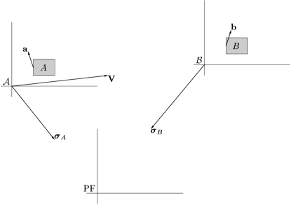
Figure 1: A schematic EPR experiment in moving frames. The detectors $A$ and $B$ are at rest in the frames $\mathcal{A}$ and $\mathcal{B}$, respectively. $\bm{\sigma}_{A}$ and $\bm{\sigma}_{B}$ denote the velocities of PF with respect to $\mathcal{A}$ and $\mathcal{B}$, respectively; while $\mathbf{V}$ denotes the velocity of $\mathcal{B}$ with respect to $\mathcal{A}$.

We remark that it is possible to express $R_{(\Lambda(\mathbf{w}),u_{A})}$, given by Eq. (37), by these velocities as well as by the corresponding velocities in the Einstein’s synchronization with the help of Eqs. (5) because it is only a reparametrization on the level of classical parameters, so it cannot affect the quantum correlations: They are still dependent on the corresponding velocities of PF with respect to the observers. Indeed, as it was discussed in Sec. II.2, the QMs built up on the different PFs are not unitary equivalent. Thus the dependence of quantum correlation functions on the velocities of PF is unremovable because it is a pure quantum phenomenon.

Now, the correlation function (36a) is

$$C(\mathbf{a},\mathbf{b})\propto\mathbf{a}\cdot B(u_{A})\Omega^{T}(\mathbf{w},u_{A})B^{-1}(u_{B})\mathbf{b},$$ (40)

where $B$ and $\Omega$ are given by the formulas (38). Note, that the correlation function given by Eq. (40) depends on the choice of PF, i.e., the two correlation functions, say $C(\mathbf{a},\mathbf{b})$ obtained for PF with the four-velocities $u_{A}$ and $u_{B}$ with respect to the observers and $\tilde{C}(\mathbf{a},\mathbf{b})$ obtained under another choice of PF with the four-velocities $\tilde{u}_{A}$ and $\tilde{u}_{B}$ with respect to the observers, do not turn into themselves when expressing $u_{A}$ and $u_{B}$ by $\tilde{u}_{A}$ and $\tilde{u}_{B}$ or vice versa. This property, related to the above mentioned nonequivalence of QMs built on different PFs, can be used to set up the experiments testing the existence and/or identification of the quantum preferred frame.

Let us discuss some special cases of Eq. (40).

1. $\mathbf{w}=\mathbf{0}$ (i.e. $\mathbf{V}=\mathbf{0}$). In this case both measurements are performed in the same inertial frame. It follows from Eq. (40), that the correlation function has the standard nonrelativistic form in this case,

   $$C(\mathbf{a},\mathbf{b})\propto\mathbf{a}\cdot\mathbf{b}=\cos\theta_{\mathbf{a}\mathbf{b}},$$ (41)

   as it should be expected. We would like to point out that the correlation function for relativistic EPR particles calculated in Refs. Czachor (1997a, b) contains corrections of the order $(\text{particle velocity}/c)^{2}$ to Eq. (41). It would be interesting to verify both the predictions experimentally.

2. $\mathbf{u}_{A}=\mathbf{0}$ or $\mathbf{u}_{B}=\mathbf{0}$. In this case one of the observers performs his/her measurement in the preferred frame. With the help of Eqs. (40) and (39) we find that

   $$C(\mathbf{a},\mathbf{b})\propto\mathbf{a}\cdot\mathbf{b},$$ (42)

   that is, we get the standard nonrelativistic formula.

3. Let us assume that the velocities $\bm{\sigma}_{A}$ and $\bm{\sigma}_{B}$ are small, i.e. $|\bm{\sigma}_{A}|\ll 1$ and $|\bm{\sigma}_{B}|\ll 1$. Such a situation occurs if the quantum-mechanical preferred frame coincides with the CBRF and the observers’ velocities are similar to the velocity of the solar system (i.e., $|\bm{\sigma}_{A}|$ and $|\bm{\sigma}_{B}|\sim 10^{-3}$). In this case

   $$\begin{split}R_{(\Lambda(\mathbf{w}),u_{A})}&\simeq I+\frac{\mathbf{V}\otimes\bm{\sigma}_{A}^{T}-\bm{\sigma}_{A}\otimes\mathbf{V}^{T}}{2}\\ &=I+\frac{\bm{\sigma}_{A}\otimes\bm{\sigma}_{B}^{T}-\bm{\sigma}_{B}\otimes\bm{\sigma}_{A}^{T}}{2},\end{split}$$

   so

   $$C(\mathbf{a},\mathbf{b})\propto\mathbf{a}\cdot\mathbf{b}+\frac{(\mathbf{a}\times\mathbf{b})\cdot(\bm{\sigma}_{A}\times\bm{\sigma}_{B})}{2}.$$ (43)

   Here $\bm{\sigma}_{A}$, $\bm{\sigma}_{B}$ and $\mathbf{V}$ are related by the approximate formula $\bm{\sigma}_{B}\simeq\bm{\sigma}_{A}-\mathbf{V}$. In the formula (43) the velocities are given in the absolute synchronization scheme but up to the fourth-order corrections they have the same form in terms of velocities $\mathbf{V}_{E},{\bm{\sigma}_{A}}_{E},{\bm{\sigma}_{B}}_{E}$ defined in the Einstein’s synchronization scheme (as it was mentioned above the reparametrization of the classical velocities cannot affect the distinguishing of the quantum preferred frame, i.e., the quantum correlation function is still dependent on the corresponding velocities of PF with respect to the observers). The deviation from the standard formula when $\mathbf{a}$ and $\mathbf{b}$ are perpendicular is shown in the Fig. 2.

   

   Figure 2: Correlation function $C(\mathbf{a},\mathbf{b})$ given by Eq. (43) for the case when $\mathbf{a}\perp\mathbf{b}$. Here $\alpha$ is the angle between $\mathbf{a}\times\mathbf{b}$ and $\bm{\sigma}_{A}\times\bm{\sigma}_{B}$, and $\beta$ is the angle between $\bm{\sigma}_{A}$ and $\bm{\sigma}_{B}$.

   Note that it follows from Eq. (43) that the corrections to the standard formula are of the order 2 in velocities. With the identification of the preferred frame with the CBRF and $\mathcal{A}$ and $\mathcal{B}$ with the solar system these corrections are of the order $10^{-6}$. Therefore, we can imagine an experiment testing this identification based on the measurement of the quantum correlations under the condition that the vectors $\mathbf{a}$ and $\mathbf{b}$ are perpendicular. In this case the standard part of the correlation function vanishes and only the effect caused by the existence of the quantum preferred frame remains [see Eq. (43) and Fig. 2]. Now, unlike in the standard EPR experiments, we should not measure the dependence of the correlation function on the angle between the vectors $\mathbf{a}$ and $\mathbf{b}$, but rather its dependence on the change of the velocities of PF, $\bm{\sigma}_{A}$ and $\bm{\sigma}_{B}$, caused by the movement of the Earth.

4. Finally we consider the case when velocities of the preferred frame are high. Denoting $\mathbf{u}_{A}/|\mathbf{u}_{A}|=\mathbf{n}_{A}$, $\mathbf{u}_{B}/|\mathbf{u}_{B}|=\mathbf{n}_{B}$ we obtain in this case

   $$R_{(\Lambda(\mathbf{w}),u_{A})}\simeq I-\left(\mathbf{n}_{A}\otimes\mathbf{n}_{A}^{T}+\mathbf{n}_{B}\otimes\mathbf{n}_{B}^{T}+\mathbf{n}_{A}\otimes\mathbf{n}_{B}^{T}\right.\\ \left.-(1+2\mathbf{n}_{A}\cdot\mathbf{n}_{B})\mathbf{n}_{B}\otimes\mathbf{n}_{A}^{T}\right)\left(1+\mathbf{n}_{A}\cdot\mathbf{n}_{B}\right)^{-1},$$

   hence,

   $$C(\mathbf{a},\mathbf{b})\propto\mathbf{a}\cdot\mathbf{b}-\frac{1}{1+\mathbf{n}_{A}\cdot\mathbf{n}_{B}}\left[(\mathbf{a}\cdot\mathbf{n}_{A})(\mathbf{b}\cdot\mathbf{n}_{A})+(\mathbf{a}\cdot\mathbf{n}_{B})(\mathbf{b}\cdot\mathbf{n}_{B})\right.\\ \left.+(\mathbf{a}\cdot\mathbf{n}_{B})(\mathbf{b}\cdot\mathbf{n}_{A})-(1+2\mathbf{n}_{A}\cdot\mathbf{n}_{B})(\mathbf{a}\cdot\mathbf{n}_{A})(\mathbf{b}\cdot\mathbf{n}_{B})\right].$$ (44)

We point out that the simultaneity of the measurements ($t_{A}=t_{B}$) is defined in the corresponding absolute synchronization scheme related to the choice of the PF .

V Conclusions

In the framework of the Lorentz-covariant quantum mechanics with the preferred frame one can build the formalism that allows to calculate correlation function in the EPR-type experiments [see Eqs. (29) and (30)] performed in moving inertial frames. We would like to point out that our results are the exact EPR correlation functions obtained for Lorentz-covariant quantum mechanical systems in moving frames under physically acceptable conditions, i.e., taking into account the localization of the particles during the detection and using the spin operator with proper transformation properties under the action of the Lorentz group.

We applied the general result to the case of simultaneous measurements of the spin component for bipartite spin-1/2 system done by the spatially bounded detectors. The resulting correlation function is proportional to $\mathbf{a}\cdot R^{T}_{(\Lambda,u_{A})}\mathbf{b}$, where $\mathbf{a}$ and $\mathbf{b}$ are the direction vectors and $R_{(\Lambda,u_{A})}$ is the Wigner rotation matrix associated with the Lorentz transformation $\Lambda$ connecting the frames of the detectors. Next we have studied the limiting cases of this particular correlation function and have shown that in the case when both measurements are performed in the same inertial frame we obtain the standard nonrelativistic result that the correlation function is proportional to the scalar product of the direction vectors. This result also holds if one of the measurements is performed in the preferred frame. We have also found the limit of the correlation function for small velocities and shown that it leads to the correction of the second order in velocities to the standard $\mathbf{a}\cdot\mathbf{b}$ relation. On the other hand, the correlation function for the very high velocities of the PF with respect to the observers depends only on the directions of movement of the PF.

It is important to stress that the exact EPR correlation function (29) depends on the PF velocity in an essential way, i.e., this dependence cannot be removed by expressing the correlation function by classical quantities (velocities) given in the Einstein’s synchronization scheme. This means that the Lorentz-covariant quantum mechanics must distinguish a preferred frame. The above results can be used to propose a realistic experiment which can answer the question of the existence of quantum-mechanical preferred frame (and its possible identification with the CBRF). A more exhaustive discussion of this problem as well as an analysis of the subtle question concerning the synchronization of clocks in the experimental setup will be given in the forthcoming paper.