ROM-based Quantum Computation: Experimental Explorations using
Nuclear Magnetic Resonance, and Future Prospects

Abstract

ROM-based quantum computation (QC) is an alternative to oracle-based QC. It has the advantages of being less “magical”, and being more suited to implementing space-efficient computation (i.e. computation using the minimum number of writable qubits). Here we consider a number of small (one and two-qubit) quantum algorithms illustrating different aspects of ROM-based QC. They are: (a) a one-qubit algorithm to solve the Deutsch problem; (b) a one-qubit binary multiplication algorithm; (c) a two-qubit controlled binary multiplication algorithm; and (d) a two-qubit ROM-based version of the Deutsch-Jozsa algorithm. For each algorithm we present experimental verification using NMR ensemble QC. The average fidelities for the implementation were in the ranges 0.9 – 0.97 for the one-qubit algorithms, and 0.84 – 0.94 for the two-qubit algorithms. We conclude with a discussion of future prospects for ROM-based quantum computation. We propose a four-qubit algorithm, using Grover’s iterate, for solving a miniature “real-world” problem relating to the lengths of paths in a network.

I Introduction

The current excitement in, and perhaps even the existence of, the field of quantum computation NieChu00 is due to the demonstration that quantum computers can solve problems in fewer steps than classical computers Deu85 ; DeuJoz92 ; Sho94 ; Gro96 ; Gro97 . An improvement is rigorously established for the Deutsch-Josza algorithm DeuJoz92 and for Grover’s search algorithm Gro97 , while Shor’s factorization algorithm Sho94 uses exponentially fewer steps than any known classical algorithm.

It is interesting that, of the above quantum algorithms, those that are provably faster (a) are not exponentially faster, and (b) make use of an oracle. An oracle is a “black-box” that defines a function

$$f:{\mathbb{Z}}_{2^{n}}\mapsto{\mathbb{Z}}_{2^{m}}.$$ (1)

Here ${\mathbb{Z}}_{N}$ is the natural numbers modulo $N$, that is, $\{0,1,\ldots,N-1\}$. The oracle ${O}_{f}$ acts on a $n$-qubit string $|{k}\rangle$, and an $m$-qubit string $|{l}\rangle$ as follows:

$$O_{f}|{k}\rangle|{l}\rangle=|{k}\rangle|{l\oplus f(k)}\rangle,$$ (2)

where $\oplus$ represents bit-wise addition modulo 2. Note that we are defining an oracle so that it can be applied to classical bit strings as well as to qubit strings.

Although the concept of an oracle is very useful in the context of complexity theory, they are, as their name suggests, somewhat “magical” in their operation. Thus they may hide a great deal of computational complexity in one step, and for this reason can be considered “unrealistic” Pap94 . In a quantum context it has been suggested that counting oracle calls may be a poor way to study the power of algorithms BenBerBraVaz97 . Finally, it seems to us that oracle-based computing is best for studying time efficiency, rather than space efficiency.

All of these factors suggest that it is worth exploring an alternative basis for computation. In this paper we explore quantum computation based on ROM (Read-Only Memory). In an earlier paper TraNieWisAmb02 two of us and co-workers showed that a ROM-based quantum computer is more space-efficient than a ROM-based classical computer. Here space efficiency is defined in terms of the number of writable qubits required. In particular, one writable qubit is sufficient to compute any binary function of an arbitrary number of ROM bits, whereas two writable bits are needed to achieve the same. Also, for a particular one-bit function (multiplication of all the ROM bits) evidence was found to support the conjecture that one qubit can solve the problem in polynomial time, whereas three bits are required for the same.

These results indicate that ROM-based computation is ideal for demonstrating space- (and possibly time-) efficiency on small scale quantum computers. Of course, at the moment small scale quantum computers are all we have experimentally. For example, in ion traps the number of qubits that can be coherently controlled is at most four Sac00 , and in Nuclear Magnetic Resonance (NMR) experiments on ensembles of molecules, the number is at most seven KniLafMarTse00 . In this paper we explore the space-efficient quantum algorithms in Ref. TraNieWisAmb02 , as well as other ROM-based quantum algorithms, in an NMR context.

The structure of this paper is as follows. In Sec. II we review ROM-based computation as defined in Ref. TraNieWisAmb02 . In Sec. III we present the simplest space-efficient one-qubit algorithm (which solves Deutsch’s problem). Sec. IV covers the one-qubit ROM-multiplication algorithm of Ref. TraNieWisAmb02 . In Sec. V we present a two-qubit version of this, the controlled-ROM-multiplication, which is also provably more space efficient than any classical algorithm (which would require three bits). In Sec. VI we explore the Deutsch-Josza algorithm using ROM rather than an oracle. In each of the sections III–VI we present experimental results following the theory, and we discuss these results in Sec. VII. We conclude in Sec. VIII with a discussion of future prospects for ROM-based quantum computation, and in particular we propose a four-qubit demonstration of quantum computing solving a “realistic” problem (i.e. a problem that can be related to the real world and that would require more than a second of human thought to solve).

II ROM-Based Computation

We consider quantum computation using qubits, the number of which remains fixed throughout the computation. The computer evolves by the operation of gates, which implement a unitary operation on one or more qubits simultaneously. It has been shown Bar95 that a single two-qubit gate, such as the controlled-NOT gate, supplemented by all one-qubit gates, is sufficient to perform all possible quantum computations in this model. Unitary gates are of course reversible. This means that in principle the computation can be carried out without dissipation of information and hence without energy cost NieChu00 ; Lan61 .

To make a fair comparison with unitary quantum computation, we must consider reversible classical computation. As is well known, universal reversible classical computation is not possible with just one-bit and two-bit gates. Rather, a three-bit gate such as the Toffoli gate or Fredkin gate is required FreTof82 . The measurement of the state of the qubits (in the computational basis) takes place only at the end of the computation. Similarly, initialization (setting a bit to a fiducial state such as $|{0}\rangle$) is allowed only at the beginning of the computation. These stipulations are necessary to keep the computation non-dissipative.

Before proceeding, let us establish some notation. We will write the $n$-bit (or qubit) representation of a number $x\in{\mathbb{Z}}_{2^{n}}$ as $|{x}\rangle$. This is equivalent to the notation $|{x}\rangle=|{x_{n-1}}\rangle|{x_{n-2}}\rangle\ldots|{x_{1}}\rangle|{x_{0}}\rangle$, where $x=\sum_{p}x_{p}2^{p}$. In a ‘circuit’ diagram, the most significant bit (MSB), $|{x_{n-1}}\rangle$, will appear at the bottom of the diagram, and the least significant bit (LSB), $|{x_{0}}\rangle$ at the top.

We used this notation already in Eq. (2) to specify the action of an oracle which implements the function $f$ defined in Eq. (1). In ROM-based computation, the function $f$ that is the subject of the computation is implemented not by an oracle, but by its values $\{f(k):k\in{\mathbb{Z}}_{N}\}$ being stored in read-only memory. Specifically, for $f$ as defined in Eq. (1), $N\times m$ ROM bits are required to store the function. For the simple case $m=1$ (a binary function), we require $N$ bits which could be allocated as $f_{0},f_{1},\cdots,f_{N-1}$, where $f_{k}\equiv f(k)$. These ROM bits are not counted in the size of the computer. That is to say, the size of the computer is taken to be the number of additional (non-ROM) (qu)bits.

To capture the essence of read-only memory, we impose the following constraints:

1. The ROM bits $\{f_{k}:k\}$ can be prepared only in a classical state.

2. For any gate involving the writable qubits, any single ROM bit, $f_{k}$ for some $k$, may act as an additional control bit.

3. No other gates involve the ROM bits.

These three conditions together imply that the ROM bits will always remain in the same state. In finite state automata models, space-bounded computation can be discussed using Turing machines with two tapes, one of which is read-only Pap94 . This is clearly very similar to the present idea of individually-accessed ROM bits. The necessity for placing a constraint on the number of ROM bits that can act as simultaneous control bits was discussed in Ref. TraNieWisAmb02 .

The restriction to single-bit ROM access leads to a simplification in the representation of ROM in circuit diagrams of reversible computation. Rather than explicitly using “wires” to represent the ROM-bits we will simply leave a space at the top of the diagram, and write in which ROM bit (if any) is acting as the extra control bit for that gate. This suggests an alternative way to conceptualize the replacement of the oracle by ROM. An oracle is like an all-knowing person who refuses to divulge information except when asked a question in a certain way. ROM is like a committee of people who each have one bit of information but who refuse to communicate with one another except by acting individually upon a device. In this way problems in ROM-based quantum computation can be seen to have some similarities to problems in quantum communication such as in Refs. BuhCelWig98 ; BraCleTap99 ; GalHar01 .

III One qubit Solution to the Deutsch problem

III.1 Theory

The smallest quantum computer is obviously one qubit. It turns out that this, plus additional ROM bits rather than an oracle, is sufficient to solve the Deutsch problem Deu85 for any $n$. The Deutsch problem can be phrased in the following way. Given a function of the form (1) with $N=2^{n}\geq 4$ and $m=1$, find a true statement from the following list:

• $f$ is not balanced.

• $f$ is not constant.

A constant function $f$ is one for which $\sum_{k}f(k)=0$ or $N$; that is, for which $f(k)=0\;\forall\;k$ or $f(k)=1\;\forall\;k$. A balanced function $f$ is one for which $\sum_{k}f(k)=N/2$. Clearly one of (A) and (B) must be true, and they both may be true in which case either can be chosen.

Deutsch and Josza found a quantum algorithm that solved this problem using $n+1$ qubits and two oracle calls DeuJoz92 . By replacing the oracle with $2^{n}$ ROM bits, we are able to solve the problem with a single qubit and with one control from each ROM bit. If we were concerned with time-efficiency, the exponential number of “ROM calls” may seem a problem. However here we are concerned only with space-efficiency.

The one-qubit algorithm to solve this problem is very simple:

$$\begin{array}[]{cccccccccccccc}\!\!&\!\!\!\!&\!\!f_{0}\!\!&\!\!\!\!&\!\!f_{1}\!\!&\!\!\!\!&\!\!\;\cdots\;\!\!&\!\!\!\!&\!\!f_{N-1}\!\!&\!\!\!\!&\!\!\!\!&\!\!\!\!&\!\!\!\!&\!\!\vspace{-0.25ex}\\ \!\!&\!\!\!\!&\!\!|\!\!&\!\!\!\!&\!\!|\!\!&\!\!\!\!&\!\!\!\!&\!\!\!\!&\!\!|\!\!&\!\!\!\!&\!\!\!\!&\!\!\!\!&\!\!\!\!&\!\!\vspace{-0.25ex}\\ |{0}\rangle\,\!\!&\!\!\!-\!\!\!-\!\!\!&\!\!\left[{\frac{2\pi}{N}}\right]_{y}\!\!\!\!&\!\!\!-\!\!\!-\!\!\!&\!\!\left[{\frac{2\pi}{N}}\right]_{y}\!\!\!\!&\!\!\!-\!\!\!-\!\!\!&\!\!\;\cdots\;\!\!&\!\!\!-\!\!\!-\!\!\!&\!\!\left[{\frac{2\pi}{N}}\right]_{y}\!\!\!\!&\!\!\!-\!\!\!-\!\!\!&\!\!\;(\!\!\!>\!\!&\!\!\!=\!\!=\!\!\!&\!\!~{}x\end{array}.$$ (3)

The computer is prepared in the fiducial state $|{0}\rangle$. Each ROM bit, $f_{k}\in\left\{{f_{0},f_{1},\cdots,f_{N-1}}\right\}$, in turn controls (indicated by the vertical line) a rotation on the qubit with unitary operator $\left[{\frac{2\pi}{N}}\right]_{y}$. That is, the gate is implemented if and only if $f_{k}=1$. Here we are using the notation

$$\left[{\theta}\right]_{\alpha}=\exp\left[{-i(\theta/2)\sigma_{\alpha}}\right],$$ (4)

where $\sigma_{\alpha}$ are the usual $2\times 2$ Pauli matrices, with $\alpha\in\left\{{x,y,z}\right\}$. For the standard representation of these matrices, the basis states are

$$|{0}\rangle=\left({\begin{array}[]{c}1\vspace{-0.25ex}\\ 0\end{array}}\right)\;,\;\;|{1}\rangle=\left({\begin{array}[]{c}0\vspace{-0.25ex}\\ 1\end{array}}\right).$$ (5)

In Eq. (3), the measurement is represented symbolically by an eye: $\;\;(\!\!\!>\;$, and yields the result $x$, a single bit. That this is a classical piece of information is represented by the double, rather than single, wire.

If the function is constant, then either it never leaves the state $|{0}\rangle$, or it is rotated by $N\times(2\pi/N)=2\pi$ around the ${y}$ axis, returning it to the state $|{0}\rangle$. If the function is balanced, it is rotated by $(N/2)\times(2\pi/N)=\pi$ around the $y$ axis, putting it into the state $|{1}\rangle$. If it is neither balanced nor constant it will end up in a superposition of $|{0}\rangle$ and $|{1}\rangle$, so a measurement will yield either result. This computation clearly solves the Deutsch problem. If the measured state $x$ of the computer is $0$, the answer returned is (B). If the measured state is $1$, the answer returned is (A).

To show the superiority of a space-bounded quantum computer over a space-bounded classical computer we simply have to prove that a one-bit classical computer cannot solve the DJ problem. Consider the simplest case, where $n=2$, so that $f$ maps $\left\{{0,1,2,3}\right\}$ to $\left\{{0,1}\right\}$. Since the only possible one-bit gate is a NOT gate $[{\rm N}]$, which obeys $[{\rm N}]^{2}=1$, the only one bit operation for this problem is

$$[{\rm N}]^{f_{0}p_{0}+f_{1}p_{1}+f_{2}p_{2}+f_{3}p_{3}},$$ (6)

where each $p_{k}\in\left\{{0,1}\right\}$. Acting on the initial state $0$, this computes the functional $\sum p_{k}f_{k}$ modulo 2. It is trivial to prove that this functional does not distinguish between balanced and constant functions for any choice of $p_{0},p_{1},p_{2},p_{3}$.

III.2 Method

The sample used for all of the following experimental demonstrations was a 0.1M solution of heavy chloroform, ¹³C¹HCl₃, dissolved in d6-acetone, CD₃COCD₃ (for locking purposes). Chlorine isotopes ³⁵Cl and ³⁷Cl have large quadrupole moments ($I=3/2$), resulting in extremely short relaxation times when covalently bonded, on the order of $10\mu s$. This has the effect of masking scalar coupling between chlorine and other nuclei HarMan78 . Thus, the chloroform molecule is effectively a two-spin system, proton and carbon-13, with $I=1/2$ for both spins.

All spectra were obtained using a Bruker DRX-500 spectrometer, for which the magnitude of $H_{0}$ was approximately $11.6T$. The resonance frequencies of the proton peaks were $\nu_{\rm H}=500.137849$MHz and $\nu_{\rm C}=125.77754749$ MHz. The scalar coupling was measured to be $J=(214.8\pm 0.5)$Hz. Clearly, $J\ll|\nu_{\rm H}-\nu_{\rm C}|$, so that the two spins can be resonantly excited independently. There is more than $1$kHz separation to the solvent lines, which thus played no part in the experiment. All experiments were performed at a temperature of $(298\pm 0.1)$K. The measured values for the longitudinal $T_{1}$ and transverse $T_{2}^{*}$ (including field inhomogeneity effects) relaxation times were $T_{1}(\mathrm{H})=(9.7\pm 0.2)$s, $T_{1}(\mathrm{C})=(11.0\pm 0.2)$s, $T_{2}^{*}(\mathrm{H})=(6.4\pm 0.3)$s, and $T_{2}^{*}(\mathrm{C})=(0.2\pm 0.01)$s. The maximum pulse program time was approximately $20$ms, significantly less than all of the above values.

For the one qubit algorithms, the H nucleus was used as it had a far narrower linewidth. The initial state is the thermal equilibrium state, which has a small excess spin in the longitudinal direction (spin up). This pseudo-pure state CorFahHav97 has observable signal proportional to that of state $|{0}\rangle$, as desired. A one-qubit gate can be implemented by an appropriately phased transverse magnetic field pulse (or short sequence of pulses), rotating at the resonant (radio) frequency of the nucleus. If a particular gate is ROM-controlled then it is implemented only when the value of the controlling ROM bit is one. Following the complete pulse sequence, a $\pi/2$ transverse pulse is used to shift longitudinal spin into the transverse plane, where its precession will induce a signal in the RF coils (the read-out). A positive spectrum indicates an excess of spin-up populations before the read-out pulse was applied. The presence of the ¹³C nucleus, with almost equal population spin up and spin down, causes a frequency splitting of $J/2$. Thus the observed spectra for the two logical states are of the form

$$|{0}\rangle:~{}\!-\!\!\!\frac{|}{}\!\!\!-\!\!\!\frac{|}{}\!\!\!-\!~{}~{},~{}~{}~{}~{}~{}~{}|{1}\rangle:~{}\!-\!\!\!\frac{}{|}\!\!\!-\!\!\!\frac{}{|}\!\!\!-\!$$ (7)

The fidelity of the transformation is calculating by dividing the area under the spectrum by that which would have arisen from a perfect transformation of the thermal signal. Since the final readout is equivalent to the average of the results of projective measurements in the $\sigma_{z}$ basis of each member of the ensemble, the area ratio $R$ can be considered to be due to a mixture of the correct result (with probability $F$) and the incorrect result (with probability $1-F$), namely $R=F-(1-F)$. Thus the fidelity is calculated as $F=(R+1)/2$.

III.3 Results

The Deutsch problem has a deterministic output if one adds the promise that the function $f$ is either balanced or constant. In this case output (A) indicates that $f$ is constant and (B) that it is balanced. With $N=4$, this means that in effect there are only three different pulse sequences arising from the algorithm in Eq. (3): that in which all values of $f$ are zero, that in which two are one, and that in which all four are one.

The results of these three different pulse sequences are shown in Fig. 1. We see that the results agree well with the theory. The first case consists of doing nothing, so its fidelity is one, by definition. The fidelity of the other cases is calculating as described above. The average fidelity (taking into account that there are six possible ways in which the function can be balanced) is $\bar{F}=0.9$.

Figure 1: Spectra for H nucleus showing the implementation of our one-qubit solution to the Deutsch problem. The values of the four ROM bits are shown above each spectrum. The fidelities (F) are also shown.

IV One qubit multiplication

IV.1 Theory

The above results demonstrate that a one-qubit quantum computer can solve problems that no one-bit classical computer can. By adding one more classical bit, the problem can be solved (this is always true, as shown in Ref. TraNieWisAmb02 ). Moreover, there is a two-bit algorithm that is just as time efficient as our quantum algorithm above. (It uses the two bits to tally the $f_{k}$s modulo 3, and is based on the fact that if $2^{n}\textrm{ mod }3=2$ then $2^{n-1}\textrm{ mod }3=1$ and vice versa.)

In this section we consider another one-qubit algorithm, which is also impossible on a one-bit computer, and which is conjectured TraNieWisAmb02 to be more time efficient than any two-bit algorithm. It also solves a more natural problem than the DJ problem, namely to find the product of $N$ ROM bits $u_{1},\cdots u_{N}$. The quantum algorithm derived in Ref. TraNieWisAmb02 requires exactly $N^{2}$ ROM-calls for $N$ a power of two, and $O(N^{2})$ otherwise. The required number of ROM-calls $r$ for a two-bit classical computer was found by numerical search to be $r=1,3,5,9$ for $N=1,2,3,4$. It is conjectured that $r(N)$ is given by the recursion relation $r(N)=r(N-1)+2^{\lfloor N/2\rfloor}$, and there is an obvious classical algorithm requiring exactly this many ROM-calls. This formula is clearly asymptotically exponential in $n$, but is actually smaller than the $N^{2}$ ROM-calls in the quantum algorithm for $N=2$, $4$, and $8$.

In the experiment we only implemented the quantum algorithm for $N=2$ and $N=4$. The one qubit algorithm which determines $u_{1}\!\times\!u_{2}$ can be constructed as follows.

$$\begin{array}[]{cccccccccccccc}\!\!&\!\!\!\!&\!\!u_{1}\!\!&\!\!\!\!&\!\!u_{2}\!\!&\!\!\!\!&\!\!u_{1}\!\!&\!\!\!\!&\!\!u_{2}\!\!&\!\!\!\!&\!\!\!\!&\!\!\!\!&\!\!&\vspace{-0.25ex}\hfil\\ \!\!&\!\!\!\!&\!\!|\!\!&\!\!\!\!&\!\!|\!\!&\!\!\!\!&\!\!|\!\!&\!\!\!\!&\!\!|\!\!&\!\!\!\!&\!\!\!\!&\!\!\!\!&\!\!&\vspace{-0.25ex}\hfil\\ |{0}\rangle\,\!\!&\!\!\!-\!\!\!-\!\!\!&\!\!\left[{\frac{\pi}{2}}\right]_{y}\!\!\!\!&\!\!\!-\!\!\!-\!\!\!&\!\!\left[{\pi}\right]_{x}\!\!\!\!&\!\!\!-\!\!\!-\!\!\!&\!\!\left[{-\frac{\pi}{2}}\right]_{y}\!\!\!\!&\!\!\!-\!\!\!-\!\!\!&\!\!\left[{\pi}\right]_{x}\!\!\!\!&\!\!\!-\!\!\!-\!\!\!&\!\!\;(\!\!\!>\!\!&\!\!\!=\!\!=\!&u_{1}\!\times\!u_{2}\end{array}.$$ (8)

In an abuse of our notation, we will indicate the above algorithm as

$$\begin{array}[]{ccccccc}\!\!&\!\!u_{1}\!\times\!u_{2}\!\!&\!\!\vspace{-0.25ex}\\ \!\!&\!\!|\!\!&\!\!\vspace{-0.25ex}\\ \!\!&\!\!\!-\!\!\!-\!\left[{\pi}\right]_{y}\!\!\!-\!\!\!-\!\!\!&\!\!\end{array}.$$ (9)

Similarly, a gate effecting the transformation $\left[{\pm\frac{\pi}{4}}\right]_{x}$, conditional on $u_{1}\!\times\!u_{2}$, is

$$\begin{array}[]{ccccccccccccc}\!\!&\!\!u_{1}\!\!&\!\!\!\!&\!\!u_{2}\!\!&\!\!\!\!&\!\!u_{1}\!\!&\!\!\!\!&\!\!u_{2}\!\!&\!\!&&\!\!&\!\!u_{1}\!\times\!u_{2}\!\!&\!\!\vspace{-0.25ex}\\ \!\!&\!\!|\!\!&\!\!\!\!&\!\!|\!\!&\!\!\!\!&\!\!|\!\!&\!\!\!\!&\!\!|\!\!&\!\!&&\!\!&\!\!|\!\!&\!\!\vspace{-0.25ex}\\ \!-\!\!\!-\!\!\!&\!\!\left[{\pm\frac{\pi}{4}}\right]_{x}\!\!\!\!&\!\!\!-\!\!\!-\!\!\!&\!\!\left[{\pi}\right]_{y}\!\!\!\!&\!\!\!-\!\!\!-\!\!\!&\!\!\left[{\mp\frac{\pi}{4}}\right]_{x}\!\!\!\!&\!\!\!-\!\!\!-\!\!\!&\!\!\left[{\pi}\right]_{y}\!\!\!\!&\!\!\!-\!\!\!-\!&\equiv&\!\!&\!\!\!-\!\!\!-\!\left[{\pm\frac{\pi}{4}}\right]_{x}\!\!\!-\!\!\!-\!\!\!&\!\!\end{array}.$$ (10)

These operations can be combined to construct an algorithm which determines the answer $a=u_{1}\!\times\!u_{2}\!\times\!u_{3}\!\times\!u_{4}$, viz.

$$\begin{array}[]{cccccccccccccc}\!\!&\!\!\!\!&\!\!u_{1}\!\times\!u_{2}\!\!&\!\!\!\!&\!\!u_{3}\!\times\!u_{4}\!\!&\!\!\!\!&\!\!u_{1}\!\times\!u_{2}\!\!&\!\!\!\!&\!\!u_{3}\!\times\!u_{4}\!\!&\!\!\!\!&\!\!\!\!&\!\!\!\!&\!\!&\vspace{-0.25ex}\hfil\\ \!\!&\!\!\!\!&\!\!|\!\!&\!\!\!\!&\!\!|\!\!&\!\!\!\!&\!\!|\!\!&\!\!\!\!&\!\!|\!\!&\!\!\!\!&\!\!\!\!&\!\!\!\!&\!\!&\vspace{-0.25ex}\hfil\\ |{0}\rangle\,\!\!&\!\!\!-\!\!\!-\!\!\!&\!\!\left[{-\frac{\pi}{4}}\right]_{x}\!\!\!\!&\!\!\!-\!\!\!-\!\!\!&\!\!\!-\!\left[{\pi}\right]_{y}\!\!\!-\!\!\!&\!\!\!-\!\!\!&\!\!\!-\!\left[{\frac{\pi}{4}}\right]_{x}\!\!\!-\!\!\!&\!\!\!-\!\!\!&\!\!\!-\!\left[{\pi}\right]_{y}\!\!\!-\!\!\!&\!\!\!-\!\!\!&\!\!\;(\!\!\!>\!\!&\!\!\!=\!\!=\!&a\end{array}.$$ (11)

IV.2 Results

The results shown in Figs. 2 and 3 were obtained by the method outlined above. Again we see good agreement with theory. The average fidelity was $\bar{F}=0.97$ in the case of multiplying two ROM bits, and $\bar{F}=0.92$ for multiplying four ROM bits.

Figure 2: Spectra for the H nucleus for the one-qubit algorithm for multiplying two ROM bits (shown as $u_{1}u_{2}$). A small systematic error is evident in the dispersive features seen in the last case. Other details are as in Fig. 1.

Figure 3: Spectra for the H nucleus for the one-qubit algorithm for multiplying four ROM bits (shown as $u_{1}u_{2}u_{3}u_{4}$). Small systematic errors are evident in the dispersive features seen in most cases. Other details are as in Fig. 1.

V Two qubit controlled-multiplication

V.1 Theory

It is simple to generalize the above single-qubit algorithm (with a space advantage of one bit compared to classical computation) to a two-qubit algorithm also with a space advantage of one bit. This is done by requiring the calculation of $u_{1}\!\times\!u_{2}\!\times\!\cdots u_{n}\!\times\!x_{1}$, where $x_{1}$ is the value of the second writable bit. The modified algorithm is identical to the one in the preceding section, except that all of the gates (which act on the first bit $|{x_{0}}\rangle$) are controlled by the second bit $x_{1}$ as well as by all of the ROM bits. That this cannot be done on a two-bit classical computer follows from the proof by Toffoli Tof80 that multi-controlled-NOTs can not be built from single controlled-NOTs without the use of an auxiliary writable bit.

For the case $n=2$, the circuit is

$$\begin{array}[]{rcccccccccccl}\!\!&\!\!\!\!&\!\!u_{1}\!\!&\!\!\!\!&\!\!u_{2}\!\!&\!\!\!\!&\!\!u_{1}\!\!&\!\!\!\!&\!\!u_{2}\!\!&\!\!\!\!&\!\!\!\!&\!\!&\vspace{-0.25ex}\\ \!\!&\!\!\!\!&\!\!|\!\!&\!\!\!\!&\!\!|\!\!&\!\!\!\!&\!\!|\!\!&\!\!\!\!&\!\!|\!\!&\!\!\!\!&\!\!\!\!&\!\!&\vspace{-0.25ex}\\ |{0}\rangle\,\!\!&\!\!\!-\!\!\!-\!\!\!&\!\!\left[{\frac{\pi}{2}}\right]_{x}\!\!\!\!&\!\!\!-\!\!\!-\!\!\!&\!\!\left[{\pi}\right]_{y}\!\!\!\!&\!\!\!-\!\!\!-\!\!\!&\!\!\left[{-\frac{\pi}{2}}\right]_{x}\!\!\!\!&\!\!\!-\!\!\!-\!\!\!&\!\!\left[{\pi}\right]_{y}\!\!\!\!&\!\!\!-\!\!\!-\!\!\!&\!\!\;(\!\!\!>\!\!&\!\!\!=\!\!=\!&x_{1}\!\times\!u_{1}\!\times\!u_{2}\vspace{-0.25ex}\\ \!\!&\!\!\!\!&\!\!|\!\!&\!\!\!\!&\!\!|\!\!&\!\!\!\!&\!\!|\!\!&\!\!\!\!&\!\!|\!\!&\!\!\!\!&\!\!\!\!&\!\!&\vspace{-0.25ex}\\ |{x_{1}}\rangle\,\!\!&\!\!\!-\!\!\!-\!\!\!&\!\!\!-\!\!\bullet\!\!-\!\!\!&\!\!\!-\!\!\!-\!\!\!&\!\!\!-\!\!\bullet\!\!-\!\!\!&\!\!\!-\!\!\!-\!\!\!&\!\!\!-\!\!-\!\!\bullet\!\!-\!\!-\!\!\!&\!\!\!-\!\!\!-\!\!\!&\!\!\!-\!\!\bullet\!\!-\!\!\!&\!\!\!-\!\!\!-\!\!\!&\!\!\;(\!\!\!>\!\!&\!\!\!=\!\!=\!&x_{1}\end{array}.$$ (12)

Here the solid circles on the wire for the second qubit indicate that it acts as a control qubit for the relevant gate.

V.2 Method

As well as selective RF pulses tuned to the H and C nuclei, the two-qubit algorithm requires an interaction between the nuclei. This occurs simply by leaving time between the (negligibly short) pulses for the spin-spin coupling Hamiltonian

$$H=hJ\sigma_{z}^{\rm H}\sigma_{z}^{\rm C}/4$$ (13)

to act. These periods of free evolution are usually of duration $1/4J$ or $1/2J$, and are simply denoted by this time. For example,

$$\left[{\frac{1}{2J}}\right]=\exp[-iH(1/2J)/\hbar]=\frac{1}{\sqrt{2}}[1-i\sigma_{z}^{\rm H}\sigma_{z}^{\rm C}].$$ (14)

The two-qubit algorithm also requires a pure initial state. A pseudo-pure state $|{00}\rangle$ of both spins (H and C) up can be prepared from the thermal equilibrium state by a sequence of RF pulses, free evolution, and gradient pulses. The last of these effectively removes the transverse spin of the sample. That is, it diagonalizes the state matrix into the logical basis. We use the pulse sequence of Cory et al. Cor99 , but change the $[\pi/6]_{y}$ pulses for both spins into a $[-\pi/6]_{y}$ pulse. This is to ensure that the signal is that for the pseudo-pure state $|{00}\rangle$, rather than the negative signal, which corresponds to a state matrix $\propto I-|{00}\rangle\langle{00}|$, where $I$ is the $4\times 4$ identity matrix. In theory, this pseudo-pure state preparation procedure results in a signal reduction by $3/8$ compared to the original thermal equilibrium state.

The readout is done identically to the one qubit case. The correspondence between the logical states and the observed spectra is more complicated. The single resonance peak for each spin is potentially split into a doublet, at $\omega\pm\pi J$. With the NMR convention of frequency increasing from right to left, the spectral shapes for the four logical states are as follows.

$$\begin{array}[]{ccc}{\rm State}&{\rm Hydrogen}&{\rm Carbon}\\ |{00}\rangle&\!-\!\!\!-\!\!\!-\!\!\!\frac{|}{}\!\!\!-\!&\!-\!\!\!-\!\!\!-\!\!\!\frac{|}{}\!\!\!-\!\\ |{01}\rangle&\!-\!\!\!-\!\!\!-\!\!\!\frac{}{|}\!\!\!-\!&\!-\!\!\!\frac{|}{}\!\!\!-\!\!\!-\!\!\!-\!\\ |{10}\rangle&\!-\!\!\!\frac{|}{}\!\!\!-\!\!\!-\!\!\!-\!&\!-\!\!\!-\!\!\!-\!\!\!\frac{}{|}\!\!\!-\!\\ |{11}\rangle&\!-\!\!\!\frac{}{|}\!\!\!-\!\!\!-\!\!\!-\!&\!-\!\!\!\frac{}{|}\!\!\!-\!\!\!-\!\!\!-\!\end{array}$$ (15)

As in the one qubit cases, for calculating the fidelity we are interested only in the occupation of the logical states, since our computation is meant to be deterministic. We integrate under the spectra at the four frequencies, and divide by 0.375 of the area of the original thermal state. The 0.375 is due to the theoretical signal loss in the pseudo-pure state preparation described above. This procedure gives a number linearly related to the occupation probabilities $p_{00}$, $p_{10}$, $p_{01}$, and $p_{11}$. For example, the area ratio $R^{\rm H}_{l}$ under the left Hydrogen peak should satisfy

$$R^{\rm H}_{l}=p_{10}-p_{11}.$$ (16)

In addition, the probabilities should sum to unity. Thus we have five equations in four unknowns, which we solve by a least-squares method to yield the probabilities. If the desired outcome is $|{11}\rangle$, for example, then the fidelity equals $p_{11}$.

The above algorithm requires four controlled gates. These can be constructed from resonant pulses on the two nuclei, plus periods of free evolution of duration $1/2J$ or $1/4J$. Specifically,

$$\begin{array}[]{ccccccccccccccccc}\!-\!\!\!-\!\!\!&\!\!\left[{\frac{\pi}{2}}\right]_{x}\!\!\!\!&\!\!\!-\!\!\!-\!&&\!-\!\!\!-\!\!\!&\!\!\left[{\frac{\pi}{2}}\right]_{y}\!\!\!\!&\!\!\!-\!\!\!-\!\!\!&\!\!\lceil\!\!&\!\!\!\!&\!\!\rceil\!\!&\!\!\!-\!\!\!-\!\!\!&\!\!\left[{\frac{\pi}{2}}\right]_{y}\!\!\!\!&\!\!\!-\!\!\!-\!\!\!&\!\!\left[{-\frac{\pi}{4}}\right]_{x}\!\!\!\!&\!\!\!-\!\!\!-\!\!\!&\!\!\left[{-\pi}\right]_{y}\!\!\!\!&\!\!\!-\!\!\!-\!\vspace{-0.5ex}\\ \!\!&\!\!|\!\!&\!\!&=&\!\!&\!\!\!\!&\!\!\!\!&\!\!\left|\right.\!\!&\!\!\frac{1}{4J}\!\!&\!\!|\!\!&\!\!\!\!&\!\!\!\!&\!\!\!\!&\!\!\!\!&\!\!\!\!&\!\!\vspace{-0.25ex}\\ \!-\!\!\!-\!\!\!&\!\!\!-\!\!\bullet\!\!-\!\!\!&\!\!\!-\!\!\!-\!&&\!-\!\!\!-\!\!\!&\!\!\!-\!\!\!-\!\!\!-\!\!\!&\!\!\!-\!\!\!-\!\!\!&\!\!\lfloor\!\!&\!\!\!\!&\!\!\rfloor\!\!&\!\!\!-\!\!\!-\!\!\!&\!\!\!-\!\!\!-\!\!\!-\!\!\!&\!\!\!-\!\!\!-\!\!\!&\!\!\!-\!\!\!-\!\!-\!\!\!-\!\!\!-\!\!\!&\!\!\!-\!\!\!-\!\!\!&\!\!\!-\!\!\!-\!\!-\!\!\!-\!\!\!&\!\!\!-\!\!\!-\!\end{array}\;,$$ (17)

$$\begin{array}[]{ccccccccccccccc}\!-\!\!\!-\!\!\!&\!\!\left[{-\frac{\pi}{2}}\right]_{x}\!\!\!\!&\!\!\!-\!\!\!-\!&&\!-\!\!\!-\!\!\!&\!\!\left[{-\frac{\pi}{2}}\right]_{y}\!\!\!\!&\!\!\!-\!\!\!-\!\!\!&\!\!\lceil\!\!&\!\!\!\!&\!\!\rceil\!\!&\!\!\!-\!\!\!-\!\!\!&\!\!\left[{\frac{\pi}{2}}\right]_{y}\!\!\!\!&\!\!\!-\!\!\!-\!\!\!&\!\!\left[{-\frac{\pi}{4}}\right]_{x}\!\!\!\!&\!\!\!-\!\!\!-\!\vspace{-0.5ex}\\ \!\!&\!\!|\!\!&\!\!&=&\!\!&\!\!\!\!&\!\!\!\!&\!\!\left|\right.\!\!&\!\!\frac{1}{4J}\!\!&\!\!|\!\!&\!\!\!\!&\!\!\!\!&\!\!\!\!&\!\!\!\!&\!\!\vspace{-0.25ex}\\ \!-\!\!\!-\!\!\!&\!\!\!-\!\!-\!\!\bullet\!\!-\!\!-\!\!\!&\!\!\!-\!\!\!-\!&&\!-\!\!\!-\!\!\!&\!\!\!-\!\!\!-\!\!-\!\!\!-\!\!\!-\!\!\!&\!\!\!-\!\!\!-\!\!\!&\!\!\lfloor\!\!&\!\!\!\!&\!\!\rfloor\!\!&\!\!\!-\!\!\!-\!\!\!&\!\!\!-\!\!\!-\!\!\!-\!\!\!&\!\!\!-\!\!\!-\!\!\!&\!\!\!-\!\!\!-\!\!-\!\!\!-\!\!\!-\!\!\!&\!\!\!-\!\!\!-\!\end{array}\;,$$ (18)

and

$$\begin{array}[]{ccccccccccccc}\!-\!\!\!-\!\!\!&\!\!\left[{\pi}\right]_{y}\!\!\!\!&\!\!\!-\!\!\!-\!&&\!-\!\!\!-\!\!\!&\!\!\left[{\frac{\pi}{2}}\right]_{y}\!\!\!\!&\!\!\!-\!\!\!-\!\!\!&\!\!\lceil\!\!&\!\!\!\!&\!\!\rceil\!\!&\!\!\!-\!\!\!-\!\!\!&\!\!\left[{\frac{2\pi}{3}}\right]_{n}\!\!\!\!&\!\!\!-\!\!\!-\!\vspace{-0.5ex}\\ \!\!&\!\!|\!\!&\!\!&=&\!\!&\!\!\!\!&\!\!\!\!&\!\!\left|\right.\!\!&\!\!\frac{1}{2J}\!\!&\!\!|\!\!&\!\!\!\!&\!\!\!\!&\!\!\vspace{-0.25ex}\\ \!-\!\!\!-\!\!\!&\!\!\!-\!\!\bullet\!\!-\!\!\!&\!\!\!-\!\!\!-\!&&\!-\!\!\!-\!\!\!&\!\!\!-\!\!\!-\!\!\!-\!\!\!&\!\!\!-\!\!\!-\!\!\!&\!\!\lfloor\!\!&\!\!\!\!&\!\!\rfloor\!\!&\!\!\!-\!\!\!-\!\!\!&\!\!\!-\!\!\!-\!\!-\!\!\!-\!\!\!&\!\!\!-\!\!\!-\!\end{array},$$ (19)

where $n$ is an axis defined by ${\bf n}=({\bf x}+{\bf y})/\sqrt{2}$.

V.3 Results

The pseudo-pure state $|{00}\rangle$ was produced with fidelity of $0.93$. This appears as the first line of Fig. 4, which is a running of the controlled-multiplication algorithm when the ROM bits are $00$ (i.e. nothing is done). The results for the other possible ROM values appear in the next three spectra. All four of these spectra are the same, as they should be since the control (Carbon) qubit being set to zero means that $x_{0}=x_{1}\times u_{1}\times u_{2}=0$. The last four spectra are repeats of the first four, but with the control (Carbon) qubit initially rotated from $|{0}\rangle$ to $|{1}\rangle$. This state, $|{10}\rangle$, was prepared with fidelity $0.89$, as shown for the case where the ROM bits are $00$. As expected, all spectra but the last also have $x_{0}=0$, and the last shows $x_{0}=1$.

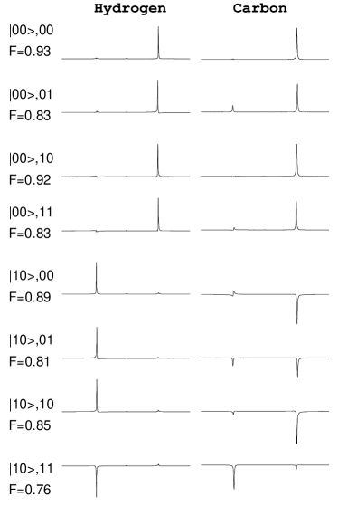
Figure 4: Spectra for the H and C nuclei for the two-qubit algorithm for multiplying two ROM bits, controlled by the first (C) bit. The initial pseudopure states of the two bits are shown with the spectra, along with the ROM bits (shown as $u_{1}u_{2}$). Small systematic errors are evident in most cases. Other details are as in Fig. 1.

The raw fidelities, calculated as discussed above, are shown on the figure. Let us scale out the fidelity of the initial state preparation (that is, divide the raw fidelities by $0.93$ for the first four spectra and $0.89$ for the second four), and take the average. Then we get a mean fidelity for the implementation of the algorithm of $\bar{F}=0.94$.

VI Two qubit ROM-based Deutsch-Josza algorithm

VI.1 Theory

We saw in Sec. III that the Deutsch Deu85 problem can be solved on a ROM-based computer with a single qubit. This algorithm was quite unlike that proposed by Deutsch Deu85 and Deutsch and Josza DeuJoz92 . In this section we investigate the implementation of the Deutsch-Josza algorithm on a ROM-based computer. This requires at least two bits to solve the Deutsch problem. Our motivations here thus do not include space efficiency. Instead, they are as follows.

First, as noted in the introduction, ROM-based computation seems more realistic, so it is interesting to see how it can be applied to an apparently quintessentially oracular algorithm.

Second, there is a question of interpretation of past experiments. Again as noted in the introduction, an oracle should be definable [see Eq. (2)] by its action on a classical computer. This is necessary in order not to give an unfair space advantage (of $m$ qubits) to a quantum computer. This requirement is met in the original theoretical proposals of Deutsch and Josza DeuJoz92 and Grover Gro97 . However, it is not met in proposals such as that in the “refined” Deutsch-Josza algorithm of Ref. ColKimHol98 , implemented in Ref. Kim99 . That is because in this algorithm the oracle directly produces phase shifts, which have no classical analogue. The requirement of Eq. (2) would also rule out the oracles implemented in other NMR experiments JonMosHan98 ; ChuGerKub98 ; Van00 (but not to those in Refs. Chu98 ; JonMos98 ; LinBarFre98 ). Our analysis here will show that these experiments can be very easily reinterpreted in terms of ROM calls rather than oracle-calls.

Third, there is a question of how quantum the Deutsch-Josza algorithm is. The use of a non-classical oracle allows the Deutsch-Josza algorithm to be implemented using one fewer qubit ($n$ rather than $n+1$). The same number ($n$) of qubits are required for the ROM-based implementation. For the minimal case $n=2$, it was shown in Ref. ColKimHol98 that with the non-classical oracle, the Deutsch-Josza algorithm does not utilize entanglement. On this basis, the authors claim that it therefore “solves the Deutsch problem in a classical way.” Leaving aside questions as to the meaning of “classical” in this context, we show that in a ROM-based implementation, entanglement necessarily occurs. This suggests that the so-called classicality noted in Ref. ColKimHol98 is due to the unrealistic nature of the oracle they use.

In the ROM-based implementation of the Deutsch-Josza algorithm, the ROM bits are the same as in Sec. III, namely the binary values $f_{0},\cdots,f_{N-1}$ of the function $f$, which is either balanced or constant. For the minimal case $N=4$ ($n=2$), the algorithm is

$$\begin{array}[]{ccccccccccccccccccccccccc}\!\!&\!\!\!\!&\!\!\!\!&\!\!\!\!&\!\!\!\!&\!\!f_{00}\!\!&\!\!\!\!&\!\!\!\!&\!\!\!\!&\!\!f_{01}\!\!&\!\!\!\!&\!\!\!\!&\!\!\!\!&\!\!f_{10}\!\!&\!\!\!\!&\!\!\!\!&\!\!\!\!&\!\!f_{11}\!\!&\!\!\!\!&\!\!\!\!&\!\!\!\!&\!\!\!\!&\!\!\!\!&\!\!&\vspace{-0.25ex}\hfil\\ \!\!&\!\!\!\!&\!\!\!\!&\!\!\!\!&\!\!\!\!&\!\!|\!\!&\!\!\!\!&\!\!\!\!&\!\!\!\!&\!\!|\!\!&\!\!\!\!&\!\!\!\!&\!\!\!\!&\!\!|\!\!&\!\!\!\!&\!\!\!\!&\!\!\!\!&\!\!|\!\!&\!\!\!\!&\!\!\!\!&\!\!\!\!&\!\!\!\!&\!\!\!\!&\!\!&\vspace{-0.25ex}\hfil\\ |{0}\rangle\,\!\!&\!\!-\!\!&\!\!\left[{\frac{\pi}{2}}\right]_{y}\!\!\!\!&\!\!\!-\!\!\!-\!\!\!&\!\!\lceil\!\!&\!\!\!\!&\!\!\rceil\!\!&\!\!\!-\!\!\!-\!\!\!&\!\!\lceil\!\!&\!\!\!\!&\!\!\rceil\!\!&\!\!\!-\!\!\!-\!\!\!&\!\!\lceil\!\!&\!\!\!\!&\!\!\rceil\!\!&\!\!\!-\!\!\!-\!\!\!&\!\!\lceil\!\!&\!\!\!\!&\!\!\rceil\!\!&\!\!\!-\!\!\!-\!\!\!&\!\!\left[{-\frac{\pi}{2}}\right]_{y}\!\!\!\!&\!\!\!-\!\!\!-\!\!\!&\!\!\;(\!\!\!>\!\!&\!\!\!=\!\!=\!&x_{0}\vspace{-0.75ex}\\ \!\!&\!\!\!\!&\!\!\!\!&\!\!\!\!&\!\!\left|\right.\!\!&\!\!\phi_{00}\!\!&\!\!|\!\!&\!\!\!\!&\!\!\left|\right.\!\!&\!\!\phi_{01}\!\!&\!\!\hskip 0.43057pt|\!\!&\!\!\!\!&\!\!\left|\right.\!\!&\!\!\phi_{10}\!\!&\!\!\hskip 0.43057pt|\!\!&\!\!\!\!&\!\!\left|\right.\!\!&\!\!\phi_{11}\!\!&\!\!|\!\!&\!\!\!\!&\!\!\!\!&\!\!\!\!&\!\!\!\!&\!\!&\vspace{-0.5ex}\hfil\\ |{0}\rangle\,\!\!&\!\!-\!\!&\!\!\left[{\frac{\pi}{2}}\right]_{y}\!\!\!\!&\!\!\!-\!\!\!-\!\!\!&\!\!\lfloor\!\!&\!\!\!\!&\!\!\rfloor\!\!&\!\!\!-\!\!\!-\!\!\!&\!\!\lfloor\!\!&\!\!\!\!&\!\!\rfloor\!\!&\!\!\!-\!\!\!-\!\!\!&\!\!\lfloor\!\!&\!\!\!\!&\!\!\rfloor\!\!&\!\!\!-\!\!\!-\!\!\!&\!\!\lfloor\!\!&\!\!\!\!&\!\!\rfloor\!\!&\!\!\!-\!\!\!-\!\!\!&\!\!\left[{-\frac{\pi}{2}}\right]_{y}\!\!\!\!&\!\!\!-\!\!\!-\!\!\!&\!\!\;(\!\!\!>\!\!&\!\!\!=\!\!=\!&x_{1}\end{array}.$$ (20)

Here the four distinct two-qubit gates, $\phi_{\alpha\beta}$ change the sign of the logical state $|{\alpha\beta}\rangle$, leaving the other three unaltered. Mathematically, the operation of these gates can be expressed as

$$\phi_{\alpha\beta}|{\gamma\delta}\rangle=(1-2\delta_{\alpha\gamma}\delta_{\beta\delta})|{\gamma\delta}\rangle$$ (21)

The result $x_{1}x_{0}=00$ indicates a constant function; any other result indicates a balanced function.

The four ROM-controlled gates together have exactly the same effect as the non-classical oracle introduced in Ref. ColKimHol98 . This is an example of how any non-classical oracle has a ROM analogue. The application of an odd number of these gates creates an entangled state, so the intermediate states of the quantum computer are entangled. It is only because the number of times the gates are applied is even (because the function is promised to be balanced or constant) that the state at the end of the four ROM-controlled gates is not entangled. Entanglement is required in all cases of this algorithm except when the function is identically zero.

VI.2 Method

We use the following realization of the two-qubit phase gates:

$$\begin{array}[]{cccccccccccccccccc}\!-\!\!\!-\!\!\!&\!\!\lceil\!\!&\!\!\!\!&\!\!\rceil\!\!&\!\!\!-\!\!\!-\!\!\!&\!\!&&\!-\!\!\!-\!\!\!&\!\!\lceil\!\!&\!\!\!\!&\!\!\rceil\!\!&\!\!\!-\!\!\!-\!\!\!&\!\!\left[{-\frac{\pi}{2}}\right]_{y}\!\!\!\!&\!\!\!-\!\!\!-\!\!\!&\!\!\left[{(-1)^{\alpha}\frac{\pi}{2}}\right]_{x}\!\!\!\!&\!\!\!-\!\!\!-\!\!\!&\!\!\left[{\frac{\pi}{2}}\right]_{y}\!\!&\!\!\!-\!\!\!-\!\vspace{-1ex}\\ \!\!&\!\!\left|\right.\!\!&\!\!\phi_{\alpha\beta}\!\!&\!\!\hskip 0.43057pt|\!\!&\!\!\!\!&\!\!&=&\!\!&\!\!\left|\right.\!\!&\!\!\frac{1}{2J}\!\!&\!\!\hskip 0.43057pt|\!\!&\!\!\!\!&\!\!\!\!&\!\!\!\!&\!\!\!\!&\!\!\!\!&\!\!\!\!&\!\!\vspace{-0.5ex}\\ \!-\!\!\!-\!\!\!&\!\!\lfloor\!\!&\!\!\!\!&\!\!\rfloor\!\!&\!\!\!-\!\!\!-\!\!\!&\!\!&&\!-\!\!\!-\!\!\!&\!\!\lfloor\!\!&\!\!\!\!&\!\!\rfloor\!\!&\!\!\!-\!\!\!-\!\!\!&\!\!\left[{-\frac{\pi}{2}}\right]_{y}\!\!\!\!&\!\!\!-\!\!\!-\!\!\!&\!\!\left[{(-1)^{\beta}\frac{\pi}{2}}\right]_{x}\!\!\!\!&\!\!\!-\!\!\!-\!\!\!&\!\!\left[{\frac{\pi}{2}}\right]_{y}\!\!\!\!&\!\!\!-\!\!\!-\!\end{array}.$$ (22)

VI.3 Results

Figure 5: Spectra for the H and C nuclei for the two-qubit ROM-based Deutsch-Josza algorithm. The ROM bits are shown as $f_{00}f_{01}f_{10}f_{11}$. Note that the order of the Carbon and Hydrogen spectra are reversed as compared to Fig. 4 and Eq. (15). Small systematic errors are evident in all cases. Other details are as in Fig. 1.

The results are shown in Fig. 5. Comparing with the table (15), we see that the result $00$ is obtained only for the case of function values $0000$ and $1111$, as expected. Results for the values $1100$, $1010$ and $0110$ were not obtained. If the algorithm implementation were perfect then the state after the four controlled phase gates in these cases would be the same as for $0011$, $0101$, and $1001$ shown in Fig. 5. There is also no reason from the pulse sequence to expect the fidelities to be very different for those cases implemented. We can thus take the cases shown as being representative, and use them to calculate an average fidelity over the eight possible functions $f$. Scaling away the fidelity of $0.93$ for the pseudo-pure state preparation (as in Sec. V), we obtain $\bar{F}=0.84$.

VII Discussion of Experimental Results

The experimental results shown clearly verify the ROM-based quantum algorithms discussed in this paper. The average fidelities of the algorithms were not unusually good for NMR experiments. They were $0.9$, $0.97$ and $0.92$ for the one qubit algorithms, and $0.94$ and $0.84$ for the two-qubit algorithms. These fidelities are definitely correlated with the length of the pulse sequence required. However, it is interesting that the lowest fidelity (0.84) was obtained for the the ROM-based Deutsch-Josza algorithm, which was not much longer than the other 2-qubit algorithm, but which differed from it in that used entangling operations.

The largest source of error was probably spatial and temporal variation in the intensity and phase of the RF pulses. The spatial variation of field strength is a direct consequence of limitations imposed by the structure of the coils, being small Helmholtz coils. Cummins and Jones CumJon00 provide a good discussion of the errors incurred in NMR computing and explain how the systematic errors due to $H_{1}$ field inhomogeneities can be greatly reduced. We did not attempt to apply these techniques.

VIII Future Prospects: A “Realistic” Problem

In this paper we have presented a number of ROM-based quantum algorithms for one- and two- qubit processors. One of these (one qubit multiplication) was derived in Ref. TraNieWisAmb02 ; the rest are new. They include a one-qubit algorithm solving the Deutsch problem, a two-qubit controlled-multiplication algorithm, and a two-qubit ROM-based Deutsch-Josza algorithm solving the Deutsch problem. For all algorithms we have also presented experimental verification, using NMR ensemble quantum computing.

All bar one of the above algorithms demonstrated space efficiency, in that a classical computer would require an extra processor bit to solve the problems. The exception is the ROM-based Deutsch-Josza algorithm. We believe that future prospects for ROM-based quantum computation lie more in the direction of this last example. There are two reasons. First, it follows from the results of Ref. TraNieWisAmb02 that the maximum space efficiency offered by ROM-based quantum computation is one bit, which could not be significant in computations of a useful scale. Second, in showing how an oracular algorithm can be implemented on a ROM-based computer, the example of Sec. VI illustrates how time-efficient quantum computing could be implemented realistically.

In the remainder of this section we will explore a future prospect for ROM-based quantum computation along these lines. We take as our basis not the Deutsch-Josza algorithm, but the other famous oracle-based algorithm, due to Grover Gro97 . We will show how the oracle in this algorithm can also be implemented using ROM-calls. We find a specific implementation with two properties of interest. First, it is experimentally feasible in the short term, requiring only four qubits. Second, it solves a problem that can be related to a read-world situation (albeit a miniaturized one), and that would require more than a second of cerebral processing time to solve.

The problem we consider relates to the lengths of paths between two vertices in a network (a set of vertices connected by edges of differing lengths). Some problems of this nature, such as finding the longest such path, are known to be NP-complete Pap94 . This is a class of problems that are almost certainly exponentially hard to solve, and are thus of great practical interest.

Consider the network below

$$\begin{array}[]{ccccc}\!\!&\!\!\!\!&\!\!U\!\!&\!\!\!\!&\!\!\vspace{-0.5ex}\\ \!\!&\!\!\nearrow\!\!&\!\!\uparrow\!\!&\!\!\searrow\!\!&\!\!\vspace{-0.5ex}\\ B\!\!&\!\!\!\!&\!\!|\!\!&\!\!\!\!&\!\!E\vspace{-0.5ex}\\ \!\!&\!\!\searrow\!\!&\!\!\downarrow\!\!&\!\!\nearrow\!\!&\!\!\vspace{-0.5ex}\\ \!\!&\!\!\!\!&\!\!L\!\!&\!\!\!\!&\!\!\end{array}~{}.$$ (23)

There are four vertices, labeled B, L, U, and E (for Begin, Lower, Upper, and End), linked by edges. These could represent cities and roads respectively. We are interested in the length of paths from B to E, as indicated by the direction of the arrows in Eq. (23). Assuming no back-tracking, there are four possible paths: BLE, BUE, BLUE, and BULE, to which we assign the numbers from 0 to 3. Each path $p$ has a length $L(p)$ associated with it, equal to the sum of the lengths $l(e)$ of each edge $e$ of the path. Six edges must be distinguished, as the edges UL and LU could well have different associated lengths. This is because “length” could represent some generalized cost, such as the time a traveler would have to wait for a lift. We discretize the problem by assuming that for all $e$, $l(e)$ is either zero or one. Thus for all $p$, $L(p)\in\{0,1,2,3\}$.

The obvious question a traveler would like to ask is, what is the shortest path? Unfortunately, this is not the sort of question that Grover’s search algorithm will answer straight away. Rather, what it can answer is questions like, what is the path of length 1? If there is exactly one path of length 1, Grover’s algorithm will find it. If there are none or two paths of length 1, Grover’s algorithm will return one of the four paths at random. If there are three paths of length 1, Grover’s algorithm will actually return the only path that is not of length 1! Thus, what Grover’s algorithm really does in our case, is to return a number $p$ which means that

path $p$, or none of the paths, is the odd-one-out with respect to having the length $L$.

Here the odd-one-out is the only one having, or the only one lacking, a property.

With a little thought it is apparent that actually we are not limited to making a demand about a specific length $L$. Rather, we can demand information about a set ${\mathbb{S}}$ of lengths $L$. Since the total length $L\in\{0,1,2,3\}$, there are seven such sets,

$${\mathbb{S}}_{1} = \{0\},$$ (24)

$${\mathbb{S}}_{2} = \{1\},$$ (25)

$${\mathbb{S}}_{3} = \{0,1\},$$ (26)

$${\mathbb{S}}_{4} = \{2\},$$ (27)

$${\mathbb{S}}_{5} = \{0,2\},$$ (28)

$${\mathbb{S}}_{6} = \{1,2\},$$ (29)

$${\mathbb{S}}_{7} = \{0,1,2\}.$$ (30)

There are other nontrivial subsets of $\{0,1,2,3\}$, but they are the complements of the above seven sets, so they would lead to demands already covered by the above seven sets. Specifically, the seven demands we could make on our computer are, with $j\in\{1,\cdots,7\}$,

What is a path $p$ such that $p$, or none of the paths, is the odd-one-out with respect to having a length $L(p)\in{\mathbb{S}}_{j}$?

In a ROM-based computation, there are six ROM bits to encode the lengths

$$l_{\rm BL},l_{\rm BU},l_{\rm LU},l_{\rm UL},l_{\rm LE},\textrm{ and }l_{\rm UE}.$$ (31)

and three to encode one of the seven sets ${\mathbb{S}}_{j}$,

$$j_{0},j_{1},\textrm{ and }j_{2},$$ (32)

where these are the bits in the binary representation of $j$. The values of the nine ROM bits thus code for 448 different instances of the general problem.

Note that the binary representation $j_{2}j_{1}j_{0}$ of $j$ is related to the set ${\mathbb{S}}_{j}$ as follows:

$${\mathbb{S}}_{j}=\{L:j_{L}=1\}$$ (33)

Using this we can construct a solution to the above problem by the following circuit:

$$\begin{array}[]{ccccccccccccccccccccccccccccccccccccccccccccccc}\!\!&\!\!\!\!&\!\!\!\!&\!\!\!\!&\!\!\!\!&\!\!l_{\rm BL}\!\!&\!\!\!\!&\!\!\!\!&\!\!\;\cdots\;\!\!&\!\!\!\!&\!\!\!\!&\!\!l_{\rm UE}\!\!&\!\!\!\!&\!\!\!\!&\!\!\!\!&\!\!j_{0}\!\!&\!\!\!\!&\!\!\!\!&\!\!\!\!&\!\!j_{1}\!\!&\!\!\!\!&\!\!\!\!&\!\!\!\!&\!\!j_{2}\!\!&\!\!\!\!&\!\!\!\!&\!\!\!\!&\!\!l_{\rm BL}\!\!&\!\!\!\!&\!\!\!\!&\!\!\;\cdots\;\!\!&\!\!\!\!&\!\!\!\!&\!\!l_{\rm UE}\!\!&\!\!\!\!&\!\!\!\!&\!\!\!\!&\!\!\!\!&\!\!\!\!&\!\!&\vspace{-0.25ex}\hfil\\ \!\!&\!\!\!\!&\!\!\!\!&\!\!\!\!&\!\!\!\!&\!\!|\!\!&\!\!\!\!&\!\!\!\!&\!\!\!\!&\!\!\!\!&\!\!\!\!&\!\!|\!\!&\!\!\!\!&\!\!\!\!&\!\!\!\!&\!\!|\!\!&\!\!\!\!&\!\!\!\!&\!\!\!\!&\!\!|\!\!&\!\!\!\!&\!\!\!\!&\!\!\!\!&\!\!|\!\!&\!\!\!\!&\!\!\!\!&\!\!\!\!&\!\!|\!\!&\!\!\!\!&\!\!\!\!&\!\!\!\!&\!\!\!\!&\!\!\!\!&\!\!|\!\!&\!\!\!\!&\!\!\!\!&\!\!\!\!&\!\!\!\!&\!\!\!\!&\!\!&\vspace{-0.25ex}\hfil\\ |{0}\rangle\,\!\!&\!\!\!-\!\!\!-\!\!\!&\!\!\!-\!\!\!-\!\!\!-\!\!\!&\!\!\!-\!\!\!-\!\!\!&\!\!\lceil\!\!&\!\!\!\!&\!\!\rceil\!\!&\!\!\!-\!\!\!-\!\!\!&\!\!\;\cdots\;\!\!&\!\!\!-\!\!\!-\!\!\!&\!\!\lceil\!\!&\!\!\!\!&\!\!\rceil\!\!&\!\!\!-\!\!\!-\!\!\!&\!\!\lceil\!\!&\!\!\!\!&\!\!\rceil\!\!&\!\!\!-\!\!\!-\!\!\!&\!\!\lceil\!\!&\!\!\!\!&\!\!\rceil\!\!&\!\!\!-\!\!\!-\!\!\!&\!\!\lceil\!\!&\!\!\!\!&\!\!\rceil\!\!&\!\!\!-\!\!\!-\!\!\!&\!\!\lceil\!\!&\!\!\!\!&\!\!\rceil\!\!&\!\!\!-\!\!\!-\!\!\!&\!\!\;\cdots\;\!\!&\!\!\!-\!\!\!-\!\!\!&\!\!\lceil\!\!&\!\!\!\!&\!\!\rceil\!\!&\!\!\!-\!\!\!-\!\!\!&\!\!|{0}\rangle\vspace{-0.5ex}\\ \!\!&\!\!\!\!&\!\!\!\!&\!\!\!\!&\!\!\left|\right.\!\!&\!\!{}\!\!&\!\!|\!\!&\!\!\!\!&\!\!\!\!&\!\!\!\!&\!\!\left|\right.\!\!&\!\!{}\!\!&\!\!|\!\!&\!\!\!\!&\!\!\left|\right.\!\!&\!\!\phi_{00}\!\!&\!\!\hskip 0.43057pt|\!\!&\!\!\!\!&\!\!\left|\right.\!\!&\!\!\phi_{01}\!\!&\!\!\hskip 0.21529pt|\!\!&\!\!\!\!&\!\!\left|\right.\!\!&\!\!\phi_{10}\!\!&\!\!\hskip 0.21529pt|\!\!&\!\!\!\!&\!\!\left|\right.\!\!&\!\!{}\!\!&\!\!|\!\!&\!\!\!\!&\!\!\!\!&\!\!\!\!&\!\!\left|\right.\!\!&\!\!{}\!\!&\!\!|\!\!&\!\!\!\!&\!\!\!\!&\!\!\!\!&\!\!&\vspace{-0.5ex}\hfil\\ |{0}\rangle\,\!\!&\!\!\!-\!\!\!-\!\!\!&\!\!\!-\!\!\!-\!\!\!-\!\!\!&\!\!\!-\!\!\!-\!\!\!&\!\!\left|\right.\!\!&\!\!\!\!&\!\!|\!\!&\!\!\!-\!\!\!-\!\!\!&\!\!\;\cdots\;\!\!&\!\!\!-\!\!\!-\!\!\!&\!\!\left|\right.\!\!&\!\!\!\!&\!\!|\!\!&\!\!\!-\!\!\!-\!\!\!&\!\!\lfloor\!\!&\!\!\!\!&\!\!\rfloor\!\!&\!\!\!-\!\!\!-\!\!\!&\!\!\lfloor\!\!&\!\!\!\!&\!\!\rfloor\!\!&\!\!\!-\!\!\!-\!\!\!&\!\!\lfloor\!\!&\!\!\!\!&\!\!\rfloor\!\!&\!\!\!-\!\!\!-\!\!\!&\!\!\left|\right.\!\!&\!\!\!\!&\!\!|\!\!&\!\!\!-\!\!\!-\!\!\!&\!\!\;\cdots\;\!\!&\!\!\!-\!\!\!-\!\!\!&\!\!\left|\right.\!\!&\!\!\!\!&\!\!|\!\!&\!\!\!-\!\!\!-\!\!\!&\!\!|{0}\rangle\vspace{-0.75ex}\\ \!\!&\!\!\!\!&\!\!\!\!&\!\!\!\!&\!\!\left|\right.\!\!&\!\!U_{\rm BL}\!\!&\!\!|\!\!&\!\!\!\!&\!\!\!\!&\!\!\!\!&\!\!\left|\right.\!\!&\!\!U_{\rm UE}\!\!&\!\!|\!\!&\!\!\!\!&\!\!\!\!&\!\!\!\!&\!\!\!\!&\!\!\!\!&\!\!\!\!&\!\!\!\!&\!\!\!\!&\!\!\!\!&\!\!\!\!&\!\!\!\!&\!\!\!\!&\!\!\!\!&\!\!\left|\right.\!\!&\!\!U^{-1}_{\rm BL}\!\!&\!\!|\!\!&\!\!\!\!&\!\!\!\!&\!\!\!\!&\!\!\left|\right.\!\!&\!\!U^{-1}_{\rm UE}\!\!&\!\!|\!\!&\!\!\!\!&\!\!\!\!&\!\!\!\!&\!\!\!\!&\!\!&\vspace{-0.5ex}\hfil\\ |{0}\rangle\,\!\!&\!\!\!-\!\!\!-\!\!\!&\!\!\left[{H}\right]\!\!&\!\!\!-\!\!\!-\!\!\!&\!\!\left|\right.\!\!&\!\!\!\!&\!\!|\!\!&\!\!\!-\!\!\!-\!\!\!&\!\!\;\cdots\;\!\!&\!\!\!-\!\!\!-\!\!\!&\!\!\left|\right.\!\!&\!\!\!\!&\!\!|\!\!&\!\!\!-\!\!\!-\!\!\!&\!\!\!-\!\!\!&\!\!\!-\!\!\!-\!\!\!-\!\!\!&\!\!\!-\!\!\!&\!\!\!-\!\!\!-\!\!\!&\!\!\!-\!\!\!&\!\!\!-\!\!\!-\!\!\!-\!\!\!&\!\!\!-\!\!\!&\!\!\!-\!\!\!-\!\!\!&\!\!\!-\!\!\!&\!\!\!-\!\!\!-\!\!\!-\!\!\!&\!\!\!-\!\!\!&\!\!\!-\!\!\!-\!\!\!&\!\!\left|\right.\!\!&\!\!\!\!&\!\!|\!\!&\!\!\!-\!\!\!-\!\!\!&\!\!\;\cdots\;\!\!&\!\!\!-\!\!\!-\!\!\!&\!\!\left|\right.\!\!&\!\!\!\!&\!\!|\!\!&\!\!\!-\!\!\!-\!\!\!&\!\!\left[{H}\right]\!\!&\!\!\!-\!\!\!-\!\!\!&\!\!\lceil\!\!&\!\!\!\!&\!\!\rceil\!\!&\!\!\!-\!\!\!-\!\!\!&\!\!\left[{H}\right]\!\!&\!\!\!-\!\!\!-\!\!\!&\!\!\;(\!\!\!>\!\!&\!\!\!=\!\!=\!&p_{0}\vspace{-0.5ex}\\ \!\!&\!\!\!\!&\!\!\!\!&\!\!\!\!&\!\!\left|\right.\!\!&\!\!\!\!&\!\!|\!\!&\!\!\!\!&\!\!\!\!&\!\!\!\!&\!\!\left|\right.\!\!&\!\!\!\!&\!\!|\!\!&\!\!\!\!&\!\!\!\!&\!\!\!\!&\!\!\!\!&\!\!\!\!&\!\!\!\!&\!\!\!\!&\!\!\!\!&\!\!\!\!&\!\!\!\!&\!\!\!\!&\!\!\!\!&\!\!\!\!&\!\!\left|\right.\!\!&\!\!\!\!&\!\!|\!\!&\!\!\!\!&\!\!\!\!&\!\!\!\!&\!\!\left|\right.\!\!&\!\!\!\!&\!\!|\!\!&\!\!\!\!&\!\!\!\!&\!\!\!\!&\!\!\left|\right.\!\!&\!\!\phi_{00}\!\!&\!\!\hskip 0.21529pt|\!\!&\!\!\!\!&\!\!\!\!&\!\!&\vspace{-0.5ex}\hfil\\ |{0}\rangle\,\!\!&\!\!\!-\!\!\!-\!\!\!&\!\!\left[{H}\right]\!\!&\!\!\!-\!\!\!-\!\!\!&\!\!\lfloor\!\!&\!\!\!\!&\!\!\rfloor\!\!&\!\!\!-\!\!\!-\!\!\!&\!\!\;\cdots\;\!\!&\!\!\!-\!\!\!-\!\!\!&\!\!\lfloor\!\!&\!\!\!\!&\!\!\rfloor\!\!&\!\!\!-\!\!\!-\!\!\!&\!\!\!-\!\!\!&\!\!\!-\!\!\!-\!\!\!-\!\!\!&\!\!\!-\!\!\!&\!\!\!-\!\!\!-\!\!\!&\!\!\!-\!\!\!&\!\!\!-\!\!\!-\!\!\!-\!\!\!&\!\!\!-\!\!\!&\!\!\!-\!\!\!-\!\!\!&\!\!\!-\!\!\!&\!\!\!-\!\!\!-\!\!\!-\!\!\!&\!\!\!-\!\!\!&\!\!\!-\!\!\!-\!\!\!&\!\!\lfloor\!\!&\!\!\!\!&\!\!\rfloor\!\!&\!\!\!-\!\!\!-\!\!\!&\!\!\;\cdots\;\!\!&\!\!\!-\!\!\!-\!\!\!&\!\!\lfloor\!\!&\!\!\!\!&\!\!\rfloor\!\!&\!\!\!-\!\!\!-\!\!\!&\!\!\left[{H}\right]\!\!&\!\!\!-\!\!\!-\!\!\!&\!\!\lfloor\!\!&\!\!\!\!&\!\!\rfloor\!\!&\!\!\!-\!\!\!-\!\!\!&\!\!\left[{H}\right]\!\!&\!\!\!-\!\!\!-\!\!\!&\!\!\;(\!\!\!>\!\!&\!\!\!=\!\!=\!&p_{1}\vspace{-0.5ex}\\ \end{array}.$$ (34)

The first pair of Hadamard gates NieChu00 puts the $|{0000}\rangle$ state into the state

$$(1/2)\sum_{p=0}^{3}|{p}\rangle|{00}\rangle,$$ (35)

where the lower two qubits, encoding the path, are in a superposition of all four possible paths. The next six gates, conditioned on the six ROM bits storing the lengths of the edges, use the upper pair of bits to count the length of each path. For example,

$$U_{\rm BL}|{p}\rangle|{L}\rangle=|{p}\rangle|{L+\chi[\textrm{BL}\sqsubset p]}\rangle.$$ (36)

Here $\chi[H]$ is the characteristic function, equal to 1 if its argument $H$ is true, and zero otherwise, while “BL $\sqsubset p$” means “BL is an edge in path number $p$”. These functions are ‘hard-wired’ in the gate construction, as they depend only of the geometry of the network in Eq. (23), not the lengths. The addition in Eq. (36) is defined modulo 4, which is reversible on 2 bits, so that this is a well-defined gate. After all six such gates have acted, the state of the processor is

$$(1/2)\sum_{p=0}^{3}|{p}\rangle|{L(p)}\rangle.$$ (37)

Upon this superposition of all paths, and their associated lengths, we now act the sign change that is at the heart of Grover’s algorithm. The three gates controlled by $j=4j_{2}+2j_{1}+j_{0}$ produce the overall phase shift

$$|{p}\rangle|{L}\rangle\to\left({1-2\chi[L\in{\mathbb{S}}_{j}]}\right)|{p}\rangle|{L}\rangle.$$ (38)

This changes the sign of the components of the superposition (37) for which the length is in the specified set ${\mathbb{S}}_{j}$. After the application of the inverse of the six controlled gates $U_{\rm BL}\cdots U_{\rm UE}$, the processor is in the state

$$(1/2)\sum_{p=0}^{3}\left\{{1-2\chi[L(p)\in{\mathbb{S}}_{j}]}\right\}|{p}\rangle|{0}\rangle.$$ (39)

Past experimental implementations of Grover’s algorithm JonMosHan98 ; ChuGerKub98 ; Van00 have relied upon a non-classical oracle that takes the processor directly from a state like Eq. (35) to one like Eq. (39). In that case, the upper pair of qubits in Eq. (34) are of course superfluous. For these experiments, where there is no real problem being solved, such an oracle seems reasonable enough. However, in the context of the present problem, which relates to a “real-world” situation — the network (23) — an oracle like this would indeed be magical. The point of the above analysis is to show that, with the help of just two additional qubits, the required oracle can nevertheless be implemented in a realistic manner, using ROM-calls.

A Grover iterate is complete with the application of Hadamard gates to the lower pair of qubits, and a phase change to the $|{00}\rangle$ state fnDJ . In this case, because the number of paths is four, a single Grover iterate suffices. The final step of the algorithm is to apply the Hadamard gates again. After this, the state of the lower pair of qubits of the processor is $|{p_{j}}\rangle$, where $p=p_{j}$ is the unique solution of $L(p)\in{\mathbb{S}}_{j}$ or $L(p)\in\bar{\mathbb{S}}_{j}$, where $\bar{\mathbb{S}}_{j}$ is the complement of ${\mathbb{S}}_{j}$. If neither of these equations have a unique solution, then the final state is a superposition of all possible paths, as in Eq. (35). Thus it is apparent that this algorithm does indeed fulfill a demand of the form above.

The above algorithm is certainly not space-efficient. From the results of Ref. TraNieWisAmb02 it follows that even a classical computer could solve this problem with a two-bit processor (although probably in more steps). Nor do we claim that it is time-efficient. A classical four-bit processor may well be able to solve the problem in fewer steps. However it would be interesting to determine what the effect would be if one stipulated that the three demand-specifying ROM-bits (the bits of $j$) only be used once, as in the above quantum algorithm. A similar ‘once-only’ constraint on information access was considered in Ref. GalHar01

A lack of both time and space efficiency for this particular algorithm would not render it worthless. Consider the one-qubit ROM-multiplication algorithm in Sec. IV. The specific instances of that algorithm we discussed and experimentally implemented were not time-efficient. However, when scaled up to larger numbers of ROM bits, the algorithm was (we conjectured) time-efficient compared to the minimal (two-bit) classical processor needed to solve this problem. Similarly, for large problems, a suitable generalization of this ROM-based Grover algorithm would, we hope, become quadratically time-efficient compared to any classical algorithm.

If Grover’s algorithm cannot be applied to “real-world” problems in this way, then it is of very limited utility. Arguments pointing to the generality of its quadratic speed up for large problems have been made by two groups. First, Brassard, Høyer and Tapp BraHoyTap98 showed how Grover’s algorithm can work even if the number of “marked” elements is unknown. Second, Cerf, Grover and Williams CerGroWil00 claimed that Grover’s algorithm can make use of the structure of a large scale problem in the same way as classical search algorithms, and thus maintain a quadratic speed up. However, serious doubts on this matter have also been expressed Zal00 , so the question remains open.

Experimentally implementing the above four-qubit algorithm is well beyond the scope of this study. We have not even compiled it into the appropriate “machine language” (NMR pulse sequences). However, this could be done along the same lines as the other algorithms presented here, by first decomposing the four-qubit gates in Eq. (34) into sequences of one and two-qubit gates. We hope that the challenge of experimental implementation on this, or some similar algorithm, is taken up. Although it would still be only a toy calculation, it would be a significant step on the way towards full-scale calculations of difficult problems pertaining to real-world situations.

- (1) M. A. Nielsen and I. L. Chuang, Quantum Computation and Quantum Information (Cambridge University Press, 2000).
- (2) D. Deutsch, Proc. R. Soc. Lond. A 400, 97 (1985).
- (3) D. Deutsch and R. Josza, Proc. R. Soc. Lond. A 439, 553 (1992).
- (4) P. W. Shor, Proc. of the 35th Annual Symposium on the Foundations of Computer Science, pp.124-134, IEEE Computer Society Press (1994).
- (5) L. K. Grover, Proc. of the 28th Annual ACM Symposium on the Theory of Computing, (Philadelphia, Penn., May 1996) pp. 212-219.
- (6) L. K. Grover, Phys. Rev. Lett. 79, 325 (1997).
- (7) C. H. Papadimitriou Computational Complexity (Addison-Wesley, Massachusetts, 1994).
- (8) C. H. Bennett, E. Bernstein, G. Brassard and U. Vazirani, SIAM J. Comput. 26, 4709 (1997).
- (9) B. C. Travaglione, M. A. Nielsen, H. M. Wiseman, and A. Ambainis, quant-ph/0109016.
- (10) C. A. Sackett et al., Nature. 404, 256 (2000).
- (11) E. Knill, R. Laflamme, R. Martinez, and C. H. Tseng, Nature. 404, 368 (2000).
- (12) A. Barenco et al., Phys. Rev. A 52, 3457 (1995).
- (13) R. Landauer, IBM J. Res. Dev. 5, 183 (1961).
- (14) E. Fredkin and T. Toffoli, Int. J. Theo. Phys. 21, 219 (1982).
- (15) H. Buhrman, R. Cleve, and A. Wigderson, Proceedings of the Thirtieth Annual ACM Symposium on Theory of Computing. (ACM, New York, NY, USA), 63-8 (1998); quant-ph/9802040
- (16) G. Brassard, R. Cleve, and A. Tapp, Phys. Rev. Lett. 83, 1874 (1999).
- (17) E. F. Galvão and L. Hardy, quantu-ph/0110166.
- (18) T. Toffoli, in Automata, Languages and Programming, ed. by J.W. de Bakker and J. can Leeuwen (1980), p.632.
- (19) R. K. Harris and B. E. Mann, NMR and the Periodic Table, (Academic Press, London, 1978).
- (20) D. Cory, A. Fahmy, and T. Havel, Proc. Nat. Acad. Sci. 94, 1634 (1997).
- (21) D. G. Cory et al., Concepts in Magnetic Resonance 111, 225 (1999).
- (22) D. Collins, K. Kim, and W. Holton Phys. Rev. A 58, R1633 (1998).
- (23) J. Kim, J-S. Lee, S. Lee, C. Cheong Phys. Rev. A 62, 022312 (2000). (2000)
- (24) J. Jones, M. Mosca, and R. Hansen Nature 393, 344 (1998).
- (25) I. Chuang, N. Gershenfeld, and M. Kubinec Phys, Rev. Lett. 80, 3408 (1998).
- (26) L. Vandersypen et al. Appl. Phys. Lett. 76, 646 (2000)
- (27) I. Chuang et al., Nature 393, 143 (1998).
- (28) J. A. Jones and M. Mosca, J. Chem. Phys. 109, 1648 (1998).
- (29) N. Linden, H. Barjat, and R. Freeman, Chem. Phys. Lett. 296, 61 (1998).
- (30) H. K. Cummins and J. A. Jones, New J. Phys. 2, 6 (2000).
- (31) It is interesting to note that if these steps are omitted, the algorithm constructed above will still answer certain questions. They are questions like that of the Deutsch-Josza problem, giving information like “the number of paths having lengths in is not two”.
- (32) G. Brassard, P. Høyer, and A. Tapp, Proceedings of Automata, Languages and Programming, 25th International Colloquium. (Springer-Verlag, Berlin, 1998), p.820-31.
- (33) N. J. Cerf, L. K. Grover, and C. P. Williams, Phys. Rev. A 61, 032303 (2000).
- (34) C. Zalka, Phys. Rev. A 62, 052305 (2000).