Squeezing and feedback

Abstract

Electro-optical feedback has many features in common with optical nonlinearities and hence is relevant to the generation of squeezing. First, I discuss theoretical and experimental results for traveling-wave feedback, emphasizing how the “in-loop” squeezing (also known as “squashing”) differs from free squeezing. Although such feedback, based on ordinary (demolition) photodetection cannot create free squeezing, it can be used to manipulate it. Then I treat feedback based on nonlinear quantum optical measurements (of which non-demolition measurements are one example). These are able to produce free squeezing, as shown in a number of experiments. Following that I discuss theories showing that intracavity squeezing can be increased using ordinary feedback, and produced using QND-based feedback. Finally, I return to “squashed” fields and present recent results showing that the reduced in-loop fluctuations can suppress atomic decay in a manner analogous to the effect for squeezed fields.

1 Introduction

In its broadest conception, feedback could be defined to be any mechanism by which a system acts upon itself, via an intermediate system. This definition would classify, for example, a nonlinear refractive index as feedback on a beam of light. The light polarizes the medium in which it is propagating, which then affects the propagation of the light in that medium. If one is interested in the light as a quantum system, then such feedback can be modeled by modifying the Hamiltonian for the field. This is a well-known mechanism for generating squeezed states of light [1].

In this chapter I am concerned with a different concept of feedback, in which the intermediate system is external to the system of interest. That is to say, the system is an open system, in constant interaction with its environment. Feedback will occur if the change in the environment due to the system is significant in affecting the system’s dynamics. Since an environment is by definition large compared to the system, it is usual for this feedback to be ignored. This is the essence of the Born, or perturbative, approach to open systems [2]. However, the system’s environment can be deliberately engineered so that the feedback is important.

One obvious way to achieve this is for the environment to include a measurement apparatus which detects the influence of the system on its surroundings, a device to amplify this measurement, and a mechanism by which this amplified signal controls the dynamics of the system. It is also possible to engineer a feedback mechanism which does not involve a measurement device, but rather some more direct form of back-coupling from the environment to the system. In classical mechanics it is a moot point whether a device is designated a “measurement apparatus”. However in quantum mechanics the special role of measurement implies that the direct back-coupling may be quite distinct from feedback via measurement [3]. This is one reason why a peculiarly quantum theory of feedback is necessary, and interesting. In this chapter I will be concerned only with measurement-based feedback.

The history of feedback in quantum optics goes back to the observation of sub-shot-noise fluctuations in an in-loop photocurrent in the mid 1980’s by two groups [4, 5]. The theory of this phenomenon was soon addressed by Yamamoto and co-workers [6, 7], and Shapiro et al [8]. The central question they were addressing was whether this feedback was producing real squeezing, a question whose answer is not as straightforward as might be thought. These treatments were based in the Heisenberg picture and used quantum Langevin equations [2] where necessary to describe the evolution of system operators. They treated the quantum noise only within a linearized approximation. Although this approximation is probably valid for all quantum optical feedback experiments performed so far, it would not be valid in the “deep quantum” regime involving few photons and non-perturbative couplings, as is being explored in the so-called “cavity quantum electrodynamics” experiments [9].

More recently an alternative approach to quantum feedback has been proposed by myself and Milburn [10, 11], and developed fully by myself [12]. This is based on the theory of quantum trajectories [13, 14, 15], which is an application of quantum measurement theory to continuously monitored open quantum systems. By treating the measurement explicitly, this theory translates the quantum noise of the bath into classical noise in the record of detections. It can be shown to be equivalent to an exact (unlinearized) quantum Langevin treatment [12]. The advantage of the quantum trajectory method is that it allows arbitrary feedback to be treated by the theory, at least numerically. A particular limit of interest is that of Markovian feedback, in which the feedback dynamics can be modeled using a master equation. This result was not obtained by the authors using the quantum Langevin treatment.

A third approach [16] to feedback in quantum optics is to use the Glauber-Sudarshan $P$ function [17, 18, 19], a quasi-probability distribution. In this theory, the fields are given an essentially classical description, but negative probabilities are allowed in order to take into account quantum correlations [16]. This theory is just as easy to use as the quantum Langevin or quantum trajectory theories when the system dynamics which can be linearized. However, like the quantum Langevin approach, it is usually intractable when the linearization approximation cannot be made. I will not discuss this theory further in this chapter.

A fourth approach is to treat the electromagnetic field as a stream of point-like particles (photons) traveling at the speed of light. This is essentially a classical approach, which cannot describe phase properties of the fields, but which is adequate if one is interested only in intensity statistics. Formally, the in-loop photon arrivals become a self-excited classical point process. This theory was used by Shapiro et al.[8] in addition to their quantum operator theory. Similar ideas have subsequently been used by other authors [20, 21]. Like the other three approaches mentioned above this approach is easily applicable to linearized systems, but unlike them it does not give a full quantum description of the in-loop field. Again, I will not discuss this theory further in this chapter.

In the remainder of this chapter I have alternated ‘theory’ sections, which introduce the mathematical apparatus necessary for describing quantum feedback, with ‘application’ sections, which use the theory to investigate squeezing, and, where appropriate, discuss experimental results. In both of these parallel streams the material is presented in roughly the order in which it was developed, but the two streams are not synchronous.

First I introduce continuum fields, and then show how linearization allows feedback onto those fields to be treated analytically, yielding noise spectra for in-loop and out-of-loop measurements. Next I discuss the interaction of continuum fields with a localized quantum system, giving rise to quantum Langevin equations for system operators. This theory is used to describe nonlinear measurements (such as QND measurements) of continuum fields, and feedback based on the results of these measurements. An alternative to the quantum Langevin description is one based on quantum trajectories. This is most useful for illuminating feedback onto the localized systems, and I use it to investigate intracavity squeezing. In the Markovian limit the quantum trajectory picture of feedback allows one to derive a feedback master equation. This is of most use for describing dynamics which cannot be linearized, such as that of a strongly driven two-level atom. This turns out to be precisely what is needed to revisit the question of in-loop squeezing in terms of what the atom ‘sees’.

2 Continuum Fields

2.1 Canonical Quantization

Let the fundamental field be the vector potential ${\bf A}({\bf r},t)$ in the Coulomb gauge

$$\nabla\cdot{\bf A}({\bf r},t)=0.$$ (1)

The free Lagrangian density for this field is [22]

$$\pounds=\frac{\varepsilon_{0}}{2}\left({\bf E}^{2}-c^{2}{\bf B}^{2}\right),$$ (2)

where $\varepsilon_{0}$ is the permittivity of free space and $c$ is the speed of light. The electric ${\bf E}$ and magnetic ${\bf B}$ fields are defined by

$${\bf E}=-\dot{\bf A}\;;\;\;{\bf B}=\nabla\times{\bf A}.$$ (3)

From (2), the canonical field to ${\bf A}$ is $-\varepsilon_{0}{\bf E}$. Thus, in quantizing the field, these obey the canonical commutation relations

$$[A_{j}({\bf r},t),E_{k}({\bf r}^{\prime},t)]=-{i}\frac{\hbar}{\varepsilon_{0}}\delta_{jk}\delta^{3}_{\perp}({\bf r}-{\bf r}^{\prime}).$$ (4)

Here $\delta^{3}_{\perp}$ denotes a three-dimensional transverse Dirac delta-function, which is necessary to be compatible with the constraint of (1) [22]. Note that the Heisenberg picture operators in the canonical commutation relations are at equal times. In the Schrödinger picture, the same relations hold, but the time argument is omitted. The Euler-Lagrange (which is also the Heisenberg) equation of motion from (2) is the wave equation

$$\ddot{\bf A}=c^{2}\nabla^{2}{\bf A}.$$ (5)

Now consider the case of a beam of polarized light. That is to say, consider only one component $A$ of ${\bf A}$ and let its spatial variation be confined to one direction, say $z$. This simplifies the analysis, and is also appropriate for determining the inputs and outputs of a quantum optical cavity. In reality, the transverse spatial extent of the beam would be confined to some area $\Lambda$ which is determined by the area of the optical components involved [2]. However, as long as the $x$ and $y$ extensions are much greater than a wavelength, the beam can be approximated by plane waves. The appropriate wave equation is

$$\ddot{A}=c^{2}\partial_{z}^{2}{A},$$ (6)

of which I am interested only in the forward propagating solutions

$$A(z,t+t^{\prime})=A(z-ct^{\prime},t).$$ (7)

If the field is reflected off a cavity mirror (say at $z=0$) then the direction of $z$ will change at the point of reflection. This is why only one direction of propagation need be considered. The field for $z<0$ is incoming and that for $z>0$ is outgoing. The canonical commutation relation is now

$$[A(z,t),E(z^{\prime},t)]=-{i}\frac{\hbar}{\varepsilon_{0}\Lambda}\delta(z-z^{\prime}).$$ (8)

Solutions for $A$ and $E$ satisfying the wave equation (6) can be constructed using the annihilation and creation operators for the modes of frequency $\omega$, which satisfy

$$[a(\omega),a^{\dagger}(\omega^{\prime})]=\delta(\omega-\omega^{\prime}).$$ (9)

They are

$$A(z) = \sqrt{\frac{\hbar}{\varepsilon_{0}\Lambda 2\pi c}}\int_{0}^{\infty}d\omega\frac{1}{\sqrt{2\omega}}\left\{a(\omega)\exp[-{i}\omega(t-z/c)]+{\rm H.c.}\right\},$$ (10)

$$E(z) = \sqrt{\frac{\hbar}{\varepsilon_{0}\Lambda 2\pi c}}\int_{0}^{\infty}d\omega\sqrt{\frac{\omega}{2}}\left\{{i}a(\omega)\exp[-{\rm i}\omega(t-z/c)]+{\rm H.c.}\right\}.$$ (11)

This expression for the fields in terms of annihilation and creation operators for a continuum of modes defines the sense in which they are composed of photons of definite frequency. However, this sense is quite unlike the naive picture of a beam of light made up of (possibly different frequencies of) photons, hurtling through space at the speed of light. Each mode is spread over all space, so there is no way in which a photon, as an excitation of such a mode, can move at all. To define an annihilation operator $b(z,t)$ for a localized photon of a particular frequency, it would be necessary to sum many different mode operators. Such operators can be defined, with slight variations in the details of the definition [14, 23]. The various definitions are effectively equivalent in application to quantum optical problems. The authors of [14, 23] construct the localized annihilation operator from the mode annihilation operators $a(\omega)$. Here, just for variation, I am introducing a different definition for $b(z,t)$, constructed from the original fields in space-time, $A(z,t)$ and $E(z,t)$.

As established above, $A$ and $-\varepsilon_{0}E$ are canonically conjugate variables at each point in space-time. Motivated by the analogy with position and momentum, a local annihilation operator for an oscillator of angular frequency $\omega_{0}$ can be defined as

$$b(z,t)=\exp[{i}\omega_{0}(t-z/c)]\sqrt{\frac{\Lambda c}{\hbar}}\left[\sqrt{\frac{\omega_{0}\varepsilon_{0}}{2}}A(z,t)-\frac{i\varepsilon_{0}}{\sqrt{2\omega_{0}\varepsilon_{0}}}E(z,t)\right].$$ (12)

In terms of the mode operators, $b(z,t)$ is given by

$$b(z,t) = \frac{1}{\sqrt{2\pi}}\int_{0}^{\infty}d\omega\left\{\frac{\omega_{0}+\omega}{2\sqrt{\omega_{0}\omega}}a(\omega)\exp[{i}(\omega_{0}-\omega)(t-z/c)]\right.$$ (13)

$$+\left.\frac{\omega_{0}-\omega}{2\sqrt{\omega_{0}\omega}}a^{\dagger}(\omega)\exp[{i}(\omega_{0}+\omega)(t-z/c)]\right\}.$$

If the beam contains only photons of a frequency near $\omega_{0}$ then it is apparent from (13) that we can approximate $b(z,t)$ by

$$b(z,t)\approx\frac{1}{\sqrt{2\pi}}\int_{0}^{\infty}d\omega\,a(\omega)\exp[{i}(\omega_{0}-\omega)(t-z/c)].$$ (14)

From this we can calculate

$$[b(z,t),b^{\dagger}(z^{\prime},t)] \approx \frac{1}{2\pi}\int_{0}^{\infty}d\omega\exp[{i}(\omega_{0}-\omega)(z^{\prime}-z)/c]$$ (15)

$$\approx c\delta(z-z^{\prime}),$$ (16)

which explains the choice of normalization in (12). Note that the approximations involved here apply only if all of the light is at a frequency close to $\omega_{0}$. Thus, the width of the Dirac $\delta$ function in (16) should be understood to be much greater than a wavelength of light $2\pi c/\omega_{0}$.

The rotating exponential $\exp[{i}\omega_{0}(t-z/c)]$ means that a “localized photon” of frequency $\omega_{0}$ has a slowly varying annihilation operator $b(z,t)$. This operator also has the same property as the vector potential (7), obeying

$$b(z,t+t^{\prime})=b(z-ct^{\prime},t)$$ (17)

in free space. If only frequencies near $\omega_{0}$ are significantly excited, then the time-flux of energy can be easily seen to be

$$W(z,t)\simeq\hbar\omega_{0}b^{\dagger}(z,t)b(z,t).$$ (18)

Thus, the annihilation operator $b(z,t)$ conforms to one’s naive expectations, with $b^{\dagger}(z,t)b(z,t)$ being the photon flux (photons per unit time) passing $z$ at time $t$.

2.2 Photodetection

From the above discussion it should be apparent that it is not sensible to talk about a photodetector for photons of frequency $\omega_{0}$ which has a response time comparable to or smaller than $\omega_{0}^{-1}$. Therefore for practical purposes a photodetector is equivalent to an energy flux meter. In either case, as long as we are not interested in times comparable to $\omega_{0}^{-1}$, we can assume that the signal produced by an ideal photodetector at position $z_{1}$ is given by the operator

$$I(t)=b^{\dagger}_{1}(t)b_{1}(t),$$ (19)

where $b_{1}(t)\equiv b(z_{1},t)$. Here I have ignored any factors of electric charge etc. which are sometimes included but which are actually nominal.

In experiments involving lasers, it is often the case (or at least it is harmless to assume [24]) that $b_{1}(t)$ has a mean amplitude $\beta=\langle{b_{1}(t)}\rangle$. Without loss of generality, I will take $\beta$ to be real. In all that follows I will also assume that we are considering stationary statistics. That is, we are taking the long time limit of a system with a stationary state. In that case, only if the correlations of interest in the intensity of the beam of light have a characteristic time satisfying

$$\tau_{\rm cor}\gg|\beta|^{-2},$$ (20)

is it permissible to linearize (19). This means approximating it by

$$I(t)=\beta^{2}+\delta I(t)=\beta^{2}+\beta X_{1}(t),$$ (21)

where

$$X_{1}(t)=b_{1}(t)+b_{1}^{\dagger}(t)-2\beta$$ (22)

is the amplitude quadrature fluctuation operator for the continuum field. For the linearization to be valid the fluctuations must be small as well as slow:

$$\langle{X_{1}(t+\tau)X_{1}(t)}\rangle\ll\beta^{2}\textrm{ for }\tau\sim\tau_{\rm corr}.$$ (23)

It is useful also to define the phase quadrature fluctuation operator

$$Y_{1}(t)=-ib_{1}(t)+ib_{1}^{\dagger}(t).$$ (24)

For free fields, which obey (17), these obey the commutation relations

$$[X_{1}(t),Y_{1}(t^{\prime})]=2i\delta(t-t^{\prime}).$$ (25)

If we define the Fourier transformed operator

$$\tilde{X}_{1}(\omega)=\int_{-\infty}^{\infty}dtX_{1}(t)e^{-i\omega t}$$ (26)

and similarly for $\tilde{Y}_{1}(\omega)$ then

$$[\tilde{X}_{1}(\omega),\tilde{Y}_{1}(\omega^{\prime})]=4\pi i\delta(\omega+\omega^{\prime}).$$ (27)

For stationary statistics as we are considering, $\langle{X_{1}(t)X_{1}(t^{\prime})}\rangle$ is a function of $t-t^{\prime}$ only. From this it follows that

$$\langle{\tilde{X}_{1}(\omega)\tilde{X}_{1}(\omega^{\prime})}\rangle\propto\delta(\omega+\omega^{\prime}).$$ (28)

Because of the singularities in equations (27) and (28), to obtain a finite uncertainty relation it is more useful to consider the spectrum

$$S_{1}^{X}(\omega) = \frac{1}{2\pi}\int_{-\infty}^{\infty}\langle{\tilde{X}_{1}(\omega)\tilde{X}_{1}(-\omega^{\prime})}\rangle d\omega^{\prime}$$ (29)

$$= \int_{-\infty}^{\infty}e^{-i\omega t}\langle{X(t)X(0)}\rangle dt\,=\,\langle{\tilde{X}_{1}(\omega)X_{1}(0)}\rangle.$$ (30)

Then it can be shown that for a stationary free field [8],

$$S_{1}^{X}(\omega)S_{1}^{Y}(\omega)\geq 1.$$ (31)

From this it is obvious that a coherent continuum field [17, 18, 19] is one such that for all $\omega$

$$S_{1}^{Q}(\omega)=1,$$ (32)

where $Q=X$ or $Y$ (or any intermediate quadrature). This is known as the standard quantum limit or shot-noise limit. A squeezed continuum field is one such that, for some $\omega$ and some $Q$,

$$S_{1}^{Q}(\omega)<1.$$ (33)

The physical significance of $S_{1}^{X}(\omega)$ is apparent from (21): it can be experimentally determined as

$$S_{1}^{X}(\omega)=\langle{I(t)}\rangle^{-1}\int_{-\infty}^{\infty}e^{-i\omega t}\langle{I(t),I(0)}\rangle dt,$$ (34)

where $\langle{A,B}\rangle=\langle{AB}\rangle-\langle{A}\rangle\langle{B}\rangle$. In fact it is possible to determine $S_{1}^{Q}(\omega)$ for any quadrature $Q$ in a similar way. Putting the field of interest through a low-reflectivity beam splitter, while reflecting another field with a large coherent amplitude off the same beam splitter, a coherent amplitude can be added to the beam of interest. If this contribution is sufficiently large it will dominate the total coherent amplitude of the beam. Since the added component can have any chosen phase with respect to the original beam, the new linearized intensity fluctuation operator will be proportional to any chosen quadrature fluctuation operator. This technique is known as homodyne detection. In practice, balanced homodyne detection using a 50–50 beam splitter and two photodetectors is preferable, but the principle is the same [25].

3 In-loop “Squeezing”

3.1 Description of the Device

The simplest form of quantum optical feedback is shown in Fig. 1. This was the scheme considered by Shapiro et al.. In our notation, we begin with a field $b_{0}=b(z_{0},t)$ as shown in the diagram.

Figure 1: Diagram for a traveling-wave feedback experiment. Traveling fields are denoted $b$ and photocurrent fluctuations $\delta I$. The first beam splitter transmittance $\eta_{1}$ is variable, the second $\eta_{2}$ fixed. The two vacuum field inputs are denoted $\nu$ and $\mu$

We will take this field to have stationary statistics with mean amplitude $\beta$ and fluctuations

$$\mbox{$\frac{1}{2}$}[X_{0}(t)+iY_{0}(t)]=b_{0}(t)-\beta$$ (35)

characterized by arbitrary spectra $S_{0}^{X}(\omega),S_{0}^{Y}(\omega)$. This field is then passed through a beam splitter of transmittance $\eta_{1}(t)$. By unitarity, the diminution in the transmitted field by a factor $\sqrt{\eta_{1}(t)}$ must be accompanied by the addition of vacuum noise from the other port of the beam splitter [1]. The transmitted field is

$$b_{1}(t)=\sqrt{\eta_{1}(t-\tau_{1})}\,b_{0}(t-\tau_{1})+\sqrt{\bar{\eta}_{1}(t-\tau_{1})}\,\nu(t-\tau_{1}).$$ (36)

Here $\tau_{1}=(z_{1}-z_{0})/c$ and I am using the notation

$$\bar{\eta}\equiv 1-\eta.$$ (37)

The operator $\nu(t)$ represents the vacuum fluctuations. The vacuum is special case of a coherent continuum field of vanishing amplitude $\langle{\nu(t)}\rangle=0$, and so is completely characterized by its spectrum

$$S_{\nu}^{Q}(\omega)=1.$$ (38)

Since the vacuum fluctuations are uncorrelated with any other field, and have stationary statistics, the phase and time arguments for $\nu(t)$ are arbitrary.

The beam-splitter transmittance $\eta_{1}(t)$ in (36) is time-dependent. This time-dependence can be achieved experimentally by a number of means. For example, if the incoming beam is elliptically polarized then an electro-optic modulator (a device with a refractive index controlled by a current) will alter the orientation of the ellipse. A polarization-sensitive beam splitter will then control the amount of the light which is transmitted, as done, for example, in [26]. As the reader will no doubt have anticipated, the current used to control the electro-optic modulator can be derived from a later detection of the light beam, giving rise to feedback. Writing $\eta_{1}(t)=\bar{\eta}_{1}+\delta\eta_{1}(t)$, and assuming that the modulation of the transmittance is small ($\delta\eta_{1}(t)\ll\eta_{1},\bar{\eta}_{1}$), one can write

$$\sqrt{\eta_{1}(t)}=\sqrt{\eta_{1}}+(1/\sqrt{\eta_{1}})\mbox{$\frac{1}{2}$}\delta\eta_{1}(t).$$ (39)

Continuing to follow the path of the beam in Fig. 1, it now enters a second beam-splitter of constant transmittance $\eta_{2}$. The transmitted beam annihilation operator

$$b_{2}(t)=\sqrt{\eta_{2}}\,b_{1}(t-\tau_{2})+\sqrt{\bar{\eta}_{2}}\,\mu(t-\tau_{2}),$$ (40)

where $\tau_{2}=(z_{2}-z_{1})/c$ and $\mu(t)$ represents vacuum fluctuations like $\nu(t)$. The reflected beam operator is

$$b_{3}(t)=\sqrt{\bar{\eta}_{2}}\,b_{1}(t-\tau_{2})-\sqrt{\eta_{2}}\,\mu(t-\tau_{2}).$$ (41)

Using the approximation (39), the linearized quadrature fluctuation operators for $b_{2}$ are

$$X_{2}(t) = \sqrt{\eta_{2}\eta_{1}}\,X_{0}(t-T_{2})+\sqrt{\eta_{2}/\eta_{1}}\,\beta\delta\eta_{1}(t-T_{2})$$ (42)

$$+\,\sqrt{\eta_{2}\bar{\eta}_{1}}\,X_{\nu}(t-T_{2})+\sqrt{\bar{\eta}_{2}}\,X_{\mu}(t-T_{2}),$$

$$Y_{2}(t) = \sqrt{\eta_{2}\eta_{1}}\,Y_{0}(t-T_{2})+\sqrt{\eta_{2}\bar{\eta}_{1}}\,Y_{\nu}(t-T_{2})+\sqrt{\bar{\eta}_{2}}\,Y_{\mu}(t-T_{2}),$$ (43)

where $T_{2}=\tau_{2}+\tau_{1}$. Similarly for $b_{3}$ we have

$$X_{3}(t) = \sqrt{\bar{\eta}_{2}\eta_{1}}\,X_{0}(t-T_{2})+\sqrt{\bar{\eta}_{2}/\eta_{1}}\,\beta\delta\eta_{1}(t-T_{2})$$ (44)

$$+\,\sqrt{\bar{\eta}_{2}\bar{\eta}_{1}}\,X_{\nu}(t-T_{2})-\sqrt{\eta_{2}}\,X_{\mu}(t-T_{2}),$$

$$Y_{3}(t) = \sqrt{\bar{\eta}_{2}\eta_{1}}\,Y_{0}(t-T_{2})+\sqrt{\bar{\eta}_{2}\bar{\eta}_{1}}\,Y_{\nu}(t-T_{2})-\sqrt{\eta_{2}}\,Y_{\mu}(t-T_{2}).$$ (45)

The mean fields for $b_{2}$ and $b_{3}$ are $\sqrt{\eta_{1}\eta_{2}}\,\beta$ and $\sqrt{\eta_{1}\bar{\eta}_{2}}\,\beta$ respectively. Thus, if these fields are incident upon photodetectors, the respective linearized photocurrent fluctuations are, as explained in Sec. 34,

$$\delta I_{2}(t) = \sqrt{\eta_{1}\eta_{2}}\,\beta\,X_{2}(t),$$ (46)

$$\delta I_{3}(t) = \sqrt{\eta_{1}\bar{\eta}_{2}}\,\beta\,X_{3}(t).$$ (47)

Here I have assumed perfect efficiency detectors. To model inefficient detectors it is necessary to add further beam splitters, with transmittance equal to the detection efficiency, in front of the detectors. The effect of this has been considered in detail in [26, 27].

Having obtained an expression for $\delta I_{2}(t)$ we are now in a position to follow the next stage in Fig. 1 and complete the feedback loop. We set the modulation in the transmittance of the first beam-splitter to be

$$\delta\eta_{1}(t)=\frac{{g}}{\eta_{2}\beta^{2}}\int_{0}^{\infty}h(t^{\prime})\delta I_{2}(t-\tau_{0}-t^{\prime})dt^{\prime},$$ (48)

where ${g}$ is a dimensionless parameter representing the low-frequency gain of the feedback loop. The response of the feedback loop, including the electro-optic elements, is assumed to be linear for small fluctuations and is characterized by the electronic delay time $\tau_{0}$ and the response function $h(t^{\prime})$, which satisfies $h(t)=0$ for $t<0$, $h(t)\geq 0$ for $t>0$ and $\int_{0}^{\infty}h(t^{\prime})dt^{\prime}=1$.

3.2 Stability

Clearly the feedback can only affect the amplitude quadrature $X$. Putting (48) into (42) yields

$$X_{2}(t) = \sqrt{\eta_{2}\eta_{1}}\,X_{0}(t-T_{2})+{g}\int_{0}^{\infty}h(t^{\prime})X_{2}(t-T-t^{\prime})dt^{\prime}$$ (49)

$$+\,\sqrt{\eta_{2}\bar{\eta}_{1}}\,X_{\nu}(t-T_{2})+\sqrt{\bar{\eta}_{2}}\,X_{\mu}(t-T_{2}),$$

where $T=\tau_{0}+T_{2}=\tau_{0}+\tau_{1}+\tau_{2}$. This is easy to solve in Fourier space, providing that $X_{2}$ is a stationary stochastic process. This will only be the case if the feedback is stable. Using standard feedback and control theory [28], the Nyquist stability criterion is

$${\rm Re}[s]<0,$$ (50)

where $s$ is any solution of the characteristic equation

$$1-{g}H(s)\exp(-sT)=0,$$ (51)

where $H(s)$ denotes the Laplace transform $H(s)=\int_{0}^{\infty}dte^{-st}h(t)$.

First I show that a sufficient condition for stability is $|g|<1$. Looking for instability, assume that ${\rm Re}[s]>0$. Then

$$\left|H(s)e^{-sT}\right|=\left|\int_{0}^{\infty}dte^{-s(t+T)}h(t)\right|\leq\int_{0}^{\infty}dth(t)=1.$$ (52)

Thus under this assumption the characteristic equation cannot be satisfied for $|{g}|<1$, so this regime will always be stable. If ${g}>1$ then it is not difficult to show that there is a positive ${s}$ which will solve (51). Thus it is a necessary condition to have ${g}<1$. If ${g}<-1$, the stability of the feedback depends on $T$ and the shape of $h(t)$. However, it turns out that it is possible to have arbitrarily large negative low-frequency feedback (that is, ${g}\to-\infty$), for any feedback loop delay $T$, provided that $h(t)$ is broad enough. The price to be paid for strong low-frequency negative feedback is a reduction in the bandwidth of the feedback, the width of $|\tilde{h}(\omega)|^{2}$.

To see this, consider the simplest smoothing function $h(t)=\gamma e^{-\gamma t}$. The condition for marginal stability is that there is a solution to (51) for $s=i\omega$. That is,

$$1={g}\exp({-i\omega T})\frac{\gamma}{\gamma+i\omega}.$$ (53)

For the imaginary part of the right-hand side to vanish we require

$$\tan\omega T=-\omega/\gamma.$$ (54)

As we will see, for large $|{g}|$ we will require $\gamma\ll T^{-1}$ in which case the solutions on (54) can be approximated by $\omega_{n}=(2n+1)\pi/2T$. Under the same approximation we can ignore $\gamma$ compared to $\omega$ in (53) to get

$$1=-|{g}|(-i)^{2n+1}\frac{2\gamma T}{i(2n+1)\pi}.$$ (55)

Clearly for $n$ odd this cannot be satisfied and so the system will be stable. However for $n$ even we have

$$1=|{g}|\frac{2\gamma T}{(2n+1)\pi},$$ (56)

which can be satisfied (indicating marginal stability). In order to avoid this for all $n$ we require

$$\gamma<\frac{\pi}{2T|{g}|}\ll\frac{1}{T},$$ (57)

where here we see that $\gamma\ll T^{-1}$ for large negative ${g}$. Now the bandwidth of the feedback is $B\simeq 2\gamma$. Thus we have finally the approximate inequality

$$B\leq\frac{\pi}{T|{g}|},$$ (58)

which shows how a finite delay time $T$ and large negative feedback $-{g}\gg 1$ reduces the possible bandwidth of the feedback.

3.3 In-loop and Out-of-loop Spectra

Assuming then that the feedback is stable we can solve (49) for $X_{2}$ in the Fourier domain:

$$\tilde{X}_{2}(\omega)=\exp({-i\omega T_{2}})\frac{\sqrt{\eta_{2}\eta_{1}}\,\tilde{X}_{0}(\omega)+\sqrt{\eta_{2}\bar{\eta}_{1}}\,\tilde{X}_{\nu}(\omega)+\sqrt{\bar{\eta}_{2}}\,\tilde{X}_{\mu}(\omega)}{1-{g}\tilde{h}(\omega)\exp(-i\omega T)}.$$ (59)

From this the amplitude quadrature spectrum is easily found from (28) and (29) to be

$$S_{2}^{X}(\omega) = \frac{\eta_{1}\eta_{2}S_{0}^{X}(\omega)+\eta_{2}\bar{\eta}_{1}S_{\nu}^{X}(\omega)+\bar{\eta}_{2}S_{\mu}^{X}(\omega)}{|1-{g}\tilde{h}(\omega)\exp(-i\omega T)|^{2}}$$ (60)

$$= \frac{1+\eta_{1}\eta_{2}[S_{0}^{X}(\omega)-1]}{|1-{g}\tilde{h}(\omega)\exp(-i\omega T)|^{2}}.$$

From these formulae the effect of feedback is obvious: it multiplies the amplitude quadrature spectrum at a given frequency by the factor $|1-{g}\tilde{h}(\omega)\exp(-i\omega T)|^{-2}$. At low frequencies, this factor is simply $(1-{g})^{-2}$, which is why the feedback was classified on this basis into positive (${g}>0$) and negative (${g}<0$) feedback. The former will increase the noise at low frequency and the latter will decrease it. However at higher frequencies, and in particular at multiples of $\pi/T$, the sign of the feedback will reverse and ${g}<0$ will result in an increase in noise and vice-versa. This is shown clearly in the theoretical investigations of Shapiro et al.. All of these results make perfect sense in the context of classical light signals, except that in that case we would not worry about vacuum noise. This is equivalent to assuming that the original noise is far above the shot-noise limit, so that one can replace $1+\eta_{1}\eta_{2}[S_{0}^{X}(\omega)-1]$ by $\eta_{1}\eta_{2}S_{0}^{X}(\omega)$. This gives the result expected from classical signal processing: the signal is attenuated by the beam splitters and either amplified or suppressed by the feedback.

The most dramatic effect is of course for large negative feedback. For sufficiently large $-{g}$ it is clear that one can make

$$S_{2}^{X}(\omega)<1$$ (61)

for some $\omega$. This effect has been observed experimentally many times with different systems involving feedback [4, 5, 7, 29, 26, 27, 30]. Without a feedback loop this sub-shot-noise photocurrent would be seen as evidence for squeezing. However, there are a number of reasons to be very cautious about applying the word squeezing to this phenomenon. Two of these reasons are theoretical, and are discussed in the following two sub-sections. The more practical reason relates to the out-of-loop beam $b_{3}$, which I will now discuss.

From (44), the $X$ quadrature of the beam $b_{3}$ is, in the Fourier domain,

$$\tilde{X}_{3}(\omega) = \exp({-i\omega T_{2}})\left[\sqrt{\bar{\eta}_{2}\eta_{1}}\,\tilde{X}_{0}(\omega)+\sqrt{\bar{\eta}_{2}\bar{\eta}_{1}}\,\tilde{X}_{\nu}(\omega)-\sqrt{\eta_{2}}\,\tilde{X}_{\mu}(\omega)\right]$$ (62)

$$+\,\sqrt{\bar{\eta}_{2}/\eta_{2}}{g}\tilde{h}(\omega)\exp(-i\omega T)\tilde{X}_{2}(\omega).$$

Here I have substituted for $\delta\eta_{1}$ in terms of $X_{2}$. Now using the above expression (59) gives

$$\tilde{X}_{3}(\omega) = \exp({-i\omega T_{2}})\left\{\frac{\sqrt{\bar{\eta}_{2}\eta_{1}}\,\tilde{X}_{0}(\omega)+\sqrt{\bar{\eta}_{2}\bar{\eta}_{1}}\,\tilde{X}_{\nu}(\omega)}{1-{g}\tilde{h}(\omega)\exp(-i\omega T)}\right.$$ (63)

$$-\,\left.\frac{\sqrt{\eta_{2}}[1-{g}\tilde{h}(\omega)\exp(-i\omega T)/\eta_{2}]\tilde{X}_{\mu}(\omega)}{1-{g}\tilde{h}(\omega)\exp(-i\omega T)}\right\}.$$

This yields the spectrum

$$S_{3}^{X}(\omega) = \frac{1+\bar{\eta}_{2}{\eta}_{1}(S_{0}^{X}-1)}{|1-{g}\tilde{h}(\omega)\exp(-i\omega T)|^{2}}$$ (64)

$$-\frac{2{\rm Re}[{g}\tilde{h}(\omega)\exp(-i\omega T)]+{g}^{2}|\tilde{h}(\omega)|^{2}/\eta_{2}}{|1-{g}\tilde{h}(\omega)\exp(-i\omega T)|^{2}}.$$

The denominator is identical to that in the in-loop case, as are the first two terms in the numerator. But there are additional terms in the numerator which indicate that there is extra noise in the out-of-loop signal.

The expression (64) can be rewritten as

$$S_{3}^{X}(\omega)=1+\frac{\bar{\eta}_{2}{\eta}_{1}(S_{0}^{X}-1)+{g}^{2}|\tilde{h}(\omega)|^{2}\bar{\eta}_{2}/\eta_{2}}{|1-{g}\tilde{h}(\omega)\exp(-i\omega T)|^{2}}.$$ (65)

From this it is apparent that, unless the initial beam is amplitude squeezed (that is, unless $S_{0}^{X}(\omega)<1$ for some $\omega$) the out-of-loop spectrum will always be greater than the shot-noise-limit of unity. In other words, it is not possible to extract the apparent squeezing in the feedback loop by using a beam splitter. In fact, in the limit of large negative feedback (which gives the greatest noise reduction in the in-loop signal), the out-of-loop amplitude spectrum approaches a constant. Considering a frequency $\omega$ such that $\tilde{h}(\omega)\exp(-i\omega T)$ is real and positive, one finds that

$$\lim_{{g}\to-\infty}S_{3}^{X}(\omega)=\eta_{2}^{-1}.$$ (66)

Thus the more light one attempts to extract from the feedback loop, the higher above shot-noise the spectrum becomes.

This result is counter to an intuition based on classical light signals, where the effect of a beam splitter is simply to split a beam so that both outputs would have the same statistics. The reason this intuition fails is precisely because this is not all that a beam splitter does; it also introduces vacuum noise which is anticorrelated at the two output ports. The detector for beam $b_{2}$ measures the amplitude fluctuations $X_{2}$, which are a combination of the initial fluctuations $X_{0}$, and the two vacuum fluctuations $X_{\nu}$ and $X_{\mu}$. The first two of these are common to the beam $b_{3}$, but the last, $X_{\mu}$, appears with opposite sign in $X_{3}$. As the negative feedback is turned up, the first two components are successfully suppressed, but the last is actually amplified. Note that the result in (66) holds no matter how large $S_{0}(\omega)$ is compared to unity.

3.4 Commutation Relations

Under normal circumstances (without a feedback loop) one would expect a sub-shot noise amplitude spectrum to imply a super-shot-noise phase spectrum. However that is not what is found from the theory presented here. Rather, the in-loop phase quadrature spectrum is unaffected by the feedback, being equal to

$$S_{2}^{Y}(\omega)=1+\eta_{1}\eta_{2}[S_{0}^{Y}(\omega)-1].$$ (67)

It is impossible to measure this spectrum without disturbing the feedback loop because all of the light in the $b_{2}$ beam must be incident upon the photodetector in order to measure $X_{2}$. However, it is possible to measure the phase-quadrature of the out-of-loop beam by homodyne detection. This was done in [26], which verified that this quadrature is also unaffected by the feedback, with

$$S_{3}^{Y}(\omega)=1+\eta_{1}\bar{\eta}_{2}[S_{0}^{Y}(\omega)-1].$$ (68)

For simplicity, consider the case where the initial beam is coherent with $S_{0}^{X}(\omega)=S_{0}^{Y}(\omega)=1$. Then $S_{2}^{Y}(\omega)=1$ and

$$S_{2}^{Y}(\omega)S_{2}^{X}(\omega)=|1-{g}\tilde{h}(\omega)\exp(-i\omega T)|^{-2}.$$ (69)

This can clearly be less than unity. This represents a violation of the uncertainty relation (31) which follows from the commutation relations (27). In fact it is easy to show (as done first by Shapiro et al. [8]) from the solution (59) that the commutation relations (27) are false for the field $b_{2}$ and must be replaced by

$$[\tilde{X}_{2}(\omega),\tilde{Y}_{2}(\omega^{\prime})]=\frac{4\pi i\delta(\omega+\omega^{\prime})}{1-{g}\tilde{h}(\omega)\exp(-i\omega T)},$$ (70)

which explains how (69) is possible.

At first sight, this apparent violation of the canonical commutation relations would seem to be a major problem of this theory. In fact, there are no violations of the canonical commutation relations. As emphasized in Sec. 2.1, the canonical commutation relations (8) are between fields at different points in space, at the same time. It is only for free fields (traveling forward in space for an indefinite time) that one can replace the space difference $z$ with a time difference $t=z/c$. Field $b_{3}$ is such a free field, as it can be detected an arbitrarily large distance away from the apparatus. Thus its quadratures at a particular point do obey the time-difference commutation relations (25), and the corresponding Fourier domain relations (27). But the field $b_{2}$ cannot travel an indefinite distance before being detected. The time from the second beam splitter to the detector $\tau_{2}$ is a physical parameter in the feedback system.

For times shorter than the total feedback loop delay $T$ it can be shown that

$$[X_{2}(t),Y_{2}(t^{\prime})]=2i\delta(t-t^{\prime})\;\;\;{\rm for}\;\;|t-t^{\prime}|<T.$$ (71)

Now the field $b_{2}$ is only in existence for a time $\tau_{2}$ before it is detected. Because $\tau_{2}<T$, this means that the time-difference commutation relations between different parts of field $b_{2}$ are actually preserved for any time such that those parts of the field are in existence, traveling through space towards the detector. It is only at times greater than the feedback loop delay time $T$ that non-standard commutation relations hold. To summarize, the commutation relations between any of the fields at different spatial points always holds, but there is no reason to expect the time or frequency commutation relations to hold for an in-loop field. Without these relations, it is not clear how “squeezing” should be defined. Indeed, it has been suggested [31] that “squashed light” would be a more appropriate term for in-loop “squeezing” because the uncertainty has actually been squashed, rather than squeezed out of one quadrature and into another.

3.5 Semiclassical Theory

A second theoretical reason against the use of the word squeezing to describe the sub-shot-noise in-loop amplitude quadrature is that (providing beam $b_{0}$ is not squeezed), the entire apparatus can be described semiclassically. In a semiclassical description there is no noise except classical noise in the field amplitudes, and shot noise is a result of a quantum detector being driven by a classical beam of light. That such a description exists might seem surprising, given the importance of vacuum fluctuations in the explanation of the spectra in Sec. 3.3. However, the semiclassical explanation, as explored in [8, 26, 32], is even simpler.

For the fields, let us use the same symbols as before, but with a cl superscript to remind us that these are classical variables rather than operators. Then the only irreducible source of noise in the system is the shot noise at the two detectors $k=2,3$. This arises from the assumption that a classical light field of frequency $\omega_{0}$ and time-flux of energy $W^{\rm cl}$ induces photo-electron emissions as a random process at rate $W^{\rm cl}/\hbar\omega_{0}$. Here $\hbar$ appears as a universal phenomenological constant relating the output of photodetectors to the incoming light. In addition to this irreducible noise, the light field itself may have (classical) noise which is represented by the amplitude fluctuation variable $X^{\rm cl}(t)$, which is scaled in the same way as the quantum operator $X(t)$ has been.

In the linearized approximation we have been working in, the Poissonian shot-noise fluctuations can be approximated by Gaussian fluctuations, giving

$$\delta I_{k}(t)=\sqrt{I_{k}}\,[X_{k}^{\rm cl}(t)+\xi_{k}(t)],$$ (72)

where $I_{k}$ is the mean value of the photocurrent and $\xi_{k}(t)$ represents independent white-noise sources obeying

$$\langle{\xi_{k}(t^{\prime})\xi_{j}(t)}\rangle=\delta_{jk}\delta(t-t^{\prime}).$$ (73)

In our case we have $\sqrt{I_{2}}=\beta\sqrt{\eta_{1}\eta_{2}}$ and $\sqrt{I_{3}}=\beta\sqrt{\eta_{1}\bar{\eta}_{2}}$

Using the above expression (48) for $\delta\eta$, the fluctuation in the field incident on detector 2 is

$$X_{2}^{\rm cl}(t) = \sqrt{\eta_{1}\eta_{2}}\,X_{0}^{\rm cl}(t-T_{2})$$ (74)

$$+\,{g}\int_{0}^{\infty}h(t^{\prime})[X_{2}^{\rm cl}(t-T-t^{\prime})+\xi_{2}(t-T-t^{\prime})]dt^{\prime}.$$

Assuming stable feedback (the conditions are the same as before) and solving this in Fourier domain we get

$$\tilde{X}_{2}^{\rm cl}(\omega)=\frac{\exp(-i\omega T_{2})\sqrt{\eta_{2}\eta_{1}}\,\tilde{X}_{0}^{\rm cl}(\omega)+{g}\tilde{h}(\omega)\exp(-i\omega T)\tilde{\xi}_{2}(\omega)}{1-{g}\tilde{h}(\omega)\exp(-i\omega T)}.$$ (75)

But the photocurrent noise itself is proportional to

$$\tilde{X}_{2}^{\rm cl}(\omega)+\tilde{\xi}_{2}(\omega)=\frac{\exp(-i\omega T_{2})\sqrt{\eta_{2}\eta_{1}}\,\tilde{X}_{0}^{\rm cl}(\omega)+\tilde{\xi}_{2}(\omega)}{1-{g}\tilde{h}(\omega)\exp(-i\omega T)}.$$ (76)

From (34) we find the spectrum

$$S_{2}^{X}(\omega)=\frac{1+\eta_{2}\eta_{1}[S^{X}_{0}(\omega)-1]}{|1-{g}\tilde{h}(\omega)\exp(-i\omega T)|^{2}},$$ (77)

where I have defined

$$S_{0}^{X}(\omega)=1+\langle{X^{\rm cl}_{0}(0)\tilde{X}^{\rm cl}_{0}(\omega)}\rangle$$ (78)

as the spectrum which would be observed with no feedback and no beam splitters. With this identification, the expression (77) is identical with (60) derived using a quantized field.

In this formulation, the sub-shot noise of the in-loop current is no surprise at all. It is simply a result of feeding back an amplified negative version of the shot noise randomly produced at the detector so that the current at a later time will be anticorrelated with itself. The low noise is in the photocurrent only, not in the light beams which here are all completely classical. This explains why the out-of-loop detector does not produce a sub-shot noise signal. The photocurrent noise at that detector is proportional to

$$\xi_{3}(t)+X_{3}^{\rm cl}(t) = \xi_{3}(t)+\sqrt{\eta_{1}\bar{\eta}_{2}}\,X_{0}^{\rm cl}(t-T_{2})+{g}\sqrt{\bar{\eta}_{2}/\eta_{2}}$$ (79)

$$\times\,\int_{0}^{\infty}h(t^{\prime})[X_{2}^{\rm cl}(t-T-t^{\prime})+\xi_{2}(t-T-t^{\prime})]dt^{\prime}.$$

Since $\xi_{3}$ is independent of everything else, it is noise which cannot be reduced by the feedback. Only the classical noise $X_{0}^{\rm cl}$ can be reduced, and that at the expense of introducing the extra uncorrelated noise $\xi_{2}$. Calculating the spectrum $S_{X}^{3}(\omega)$ again gives the same answer as the quantum theory.

3.6 QND Measurements of In-loop Beams

On the basis of the above semiclassical theory it might be thought that all of the calculations of noise spectra made in this section relate only to the noise of photocurrents and say nothing about the noise properties of the light beams themselves. While this appears to be the case from the semiclassical theory, it is not really true, as can be seen from considering quantum non-demolition (QND) measurements [1]. In this context, a QND detector is one which can measure the intensity of light without absorbing it. Such devices cannot be described by semiclassical theory, which shows that this theory is not complete and hence cannot be expected to provide the correct intuition about the state of the light itself.

A specific model for a QND device will be considered in Sec. 5.1. Here we simply assume that a perfect QND device can measure the amplitude quadrature $X$ of a continuum field without disturbing it beyond the necessary back-action from the Heisenberg uncertainty principle. In other words, the QND device should give a read-out at time $t$ which can be represented by the operator $X(t)$. The correlations of this read-out will thus reproduce the correlations of $X(t)$. For a perfect QND measurement of $X_{2}$ and $X_{3}$, the spectrum will reproduce those of the conventional (demolition) photodetectors which measure these beams. This confirms that these detectors (assumed perfect) are indeed recording the true quantum fluctuations of the light impinging upon them.

What is more interesting is to consider a QND measurement on $X_{1}$. That is because the set up in Fig. 1 is equivalent (as mentioned above) to a set up without the second beam splitter, but instead with an in-loop photodetector with efficiency $\eta_{2}$. In this version, the beams $b_{2}$ and $b_{3}$ do not physically exist. Rather, $b_{1}$ is the in-loop beam and $X_{2}$ is the operator for the noise in the photocurrent produced by the detector. As shown above, this operator can have vanishing noise at low frequencies for ${g}\to-\infty$. However, this is not reflected in the noise in the in-loop beam, as recorded by our hypothetical QND device. Following the methods of Sec. 3.3, the spectrum of $X_{1}$ is

$$S_{1}^{X}(\omega)=\frac{1+\eta_{1}[S_{0}(\omega)-1]+{g}^{2}|\tilde{h}(\omega)|^{2}\bar{\eta}_{2}/\eta_{2}}{|1-{g}\tilde{h}(\omega)\exp(-i\omega T)|^{2}}.$$ (80)

In the limit ${g}\to-\infty$, this becomes at low frequencies

$$S_{1}^{X}(0)\to\frac{1-{\eta}_{2}}{\eta_{2}},$$ (81)

which is not zero for any detection efficiency $\eta_{2}$ finitely less than one. Indeed, for $\eta_{2}<0.5$ it is above shot-noise.

The reason that the in-loop amplitude quadrature spectrum is not reduced to zero for large negative feedback is that the feedback loop is feeding back noise $X_{\mu}(t)$ in the photocurrent fluctuation operator $X_{2}(t)$ which is independent of the fluctuations in the amplitude quadrature $X_{1}(t)$ of the in-loop light. The smaller $\eta_{2}$ is, the larger the amount of extraneous noise in the photocurrent and the larger the noise introduced into the in-loop light. In order to minimize the low-frequency noise in the in-loop light, there is an optimal feedback gain. In the case $S_{0}(\omega)=1$ (a coherent input), this is given by

$${g}_{\rm opt}=-\frac{\eta_{2}}{1-\eta_{2}},$$ (82)

giving a minimum in-loop low-frequency noise spectrum

$$S_{1}^{X}(0)_{\rm min}=1-\eta_{2}.$$ (83)

The fact that the detection efficiency does matter in the attainable in-loop squeezing shows that these are true quantum fluctuations.

3.7 A Squeezed Input

Although the feedback device discussed in this section cannot produce a free squeezed beam, it is nevertheless useful for reducing classical noise in the output beam $b_{3}$. It is easy to verify the result of [26] that if one wishes to reduce classical noise $S_{0}^{X}(\omega)-1$ at a particular frequency $\omega$, then the optimum feedback is such that

$${g}\tilde{h}(\omega)\exp(-i\omega T)=-\eta_{1}\eta_{2}[S_{0}^{X}(\omega)-1].$$ (84)

This gives the lowest noise level in the amplitude of $b_{3}$ at that frequency

$$S_{3}^{X}(\omega)_{\rm opt}=1+\frac{\bar{\eta}_{2}\eta_{1}[S_{0}^{X}(\omega)-1]}{1+\eta_{2}\eta_{1}[S_{0}^{X}(\omega)-1]}.$$ (85)

For large classical noise we have feedback proportional to $S_{0}^{X}(\omega)$ and an optimal noise value of $1/\eta_{2}$, as this approaches the limit of (66). The interesting regime [26] is the opposite one, where $S_{0}^{X}(\omega)-1$ is small, or even negative. This last case corresponds to to a squeezed input beam. Putting squeezing through a beam splitter reduces the squeezing in both output beams. In this case, with no feedback the residual squeezing in beam $b_{3}$ would be

$$S_{3}^{X}(\omega)_{\rm no}=1+\bar{\eta}_{2}\eta_{1}[S_{0}^{X}(\omega)-1],$$ (86)

which is closer to unity than $S_{0}^{X}(\omega)$. The optimal feedback (the purpose of which is to reduce noise) is, according to (84), positive. That is to say, destabilizing feedback actually puts back in beam $b_{3}$ some of the squeezing lost through the beam splitter. Since the required round-loop gain (84) is less than unity, the feedback loop remains stable.

This result highlights the nonclassical nature of squeezed fluctuations. When an amplitude squeezed beam strikes a beam splitter, the intensity at one output port is anticorrelated with that at the other, hence the need for positive feedback. Preliminary observations of this effect were reported in [33]. Of course the feedback can never put more squeezing into the beam than was present at the start. That is, $S_{3}^{X}(\omega)_{\rm opt}$ always lies between $S_{0}^{X}(\omega)$ and $S_{3}^{X}(\omega)_{\rm no}$. However, if we take the limit $\eta_{1}\to 1$ and $S_{0}^{X}(\omega)\to 0$ (perfect squeezing to begin with) then all of this squeezing can be recovered, for any $\eta_{2}$. This effect might even be of practical use for attenuating highly squeezed sources, such as those produced by laser diodes, while retaining most of the squeezing [33].

4 Quantum Langevin Equations

In the preceding section, only continuum fields were considered, with all optical and electro-optical devices being treated as classical (i.e. deterministic) systems. Often one wishes to consider feedback onto quantum systems which may introduce extra noise terms into the equations. To do this one needs a theory for describing the dynamics of localized quantum systems interacting with continuum fields. In the optical regime this theory was put on a rigorous foundation by Gardiner and Collett [23]. This theory is based on an electric-dipole coupling, and involves key approximations which rely on a rapid oscillation (at optical frequency $\omega_{0}$) of the system dipole due to the system Hamiltonian $H_{0}$. Let that dipole, in the interaction picture of $H_{0}$, be proportional to

$$c(t)\exp(-i\omega_{0}t)+c^{\dagger}(t)\exp(i\omega_{0}t).$$ (87)

Here $c$ and $c^{\dagger}$ are dimensionless Heisenberg-picture system operators, normalized so that $cc^{\dagger}|{0}\rangle=|{0}\rangle$, where $|{0}\rangle$ is the ground state of $H_{0}$.

Let the system be located at $z=0$ and consider an incoming ($z<0$) and outgoing ($z>0$) continuum field with operator $b(z,t)$ as defined previously. Then, under the rotating wave approximation [2], the dipole coupling to the field at $z=0$ can be modeled by the Hamiltonian

$$V(t)=i\sqrt{\gamma}[c(t)b^{\dagger}(0,t)-b(0,t)c^{\dagger}(t)].$$ (88)

Here $\hbar=1$ and $\gamma\ll\omega_{0}$ is the characteristic decay rate of the system. For a general interaction one would have to use both space and time arguments for the continuum field. However, the coupling considered here is strictly local. Both before ($z<0$) and after ($z>0$) the interaction, the field still freely propagates. This means that, although it is necessary to use a spatial as well as a temporal argument, the spatial argument need only have two values: before and after. In order to conform with pre-established usage [23], these values will be called in and out. The input field is defined (in the Heisenberg picture) as

$$b_{\rm in}(t)=b(0^{-},t),$$ (89)

and the output field as

$$b_{\rm out}(t)=b(0^{+},t).$$ (90)

Both of these fields obey the commutation relations

$$[b(t),b^{\dagger}(t^{\prime})]=\delta(t-t^{\prime}),$$ (91)

at least for time differences shorter than the delay time in any feedback loop.

The interaction of the external field with the system at time $t$ is described by the Hamiltonian (88). It is necessary to be careful in dealing with this because of the singular commutation relations (91). A convenient way is to use the quantum Itô stochastic calculus [23]. In the Heisenberg picture, the infinitesimal unitary transformation pertaining to the interaction at time $t$ is

$$U(t,t+dt)=\exp\left[\sqrt{\gamma}c(t)dB_{\rm in}^{\dagger}(t)-\sqrt{\gamma}c(t)^{\dagger}dB_{\rm in}(t)-iH(t)dt\right],$$ (92)

where $H$ is a system Hamiltonian representing any small perturbation on top of the free energy (such as classical driving), and

$$dB_{\rm in}(t)=b_{\rm in}(t)dt$$ (93)

is the quantum analogue of the Wiener increment [23]. Note that the field operator in the unitary transformation (92) is the bath immediately before it interacts with the system, rather than the bath at the instant it is interacting with the system. This is the appropriate operator if one treats the stochastic increment $dB_{\rm in}(t)$ in the Itô sense. This means that (92) must be expanded to second order in the increment. For an input in the vacuum state, the operator $dB_{\rm in}$ has a vanishing first order moment, and a single nonvanishing second-order moment [23]

$$dB_{\rm in}(t)dB_{\rm in}^{\dagger}(t)=dt.$$ (94)

This could be thought of as vacuum noise.

Applying the unitary transformation (92) to an arbitrary system operator $s(t)$ yields

$$s(t+dt) = U^{\dagger}(t,t+dt)s(t)U(t,t+dt)$$ (95)

$$= s+\gamma\left(c^{\dagger}sc-\mbox{$\frac{1}{2}$}c^{\dagger}cs-\mbox{$\frac{1}{2}$}sc^{\dagger}c\right)dt$$

$$-\,[-iHdt+\sqrt{\gamma}dB_{\rm in}^{\dagger}(t)c-\sqrt{\gamma}c^{\dagger}dB_{\rm in}(t),s],$$

where all system operators in (95) have the time argument $t$. This is what I will refer to as a quantum Langevin equation (QLE) for $s$. Because $dB_{\rm in}(t)$ is the bath operator before it interacts with the system, it is independent of the system operator $s(t)$. Hence one can derive

$$\langle{\dot{s}}\rangle=\left\langle\left[\gamma\left(c^{\dagger}sc-\mbox{$\frac{1}{2}$}c^{\dagger}cs-\mbox{$\frac{1}{2}$}sc^{\dagger}c\right)+i[H,s]\right]\right\rangle.$$ (96)

From this it apparent that there is a Schrödinger picture representation of the system dynamics. In this picture

$$\langle{\dot{s}(t)}\rangle={\rm Tr}[\dot{\rho}(t)s],$$ (97)

where $\rho(t)$ is the state matrix for the system which evidently obeys

$$\dot{\rho}=\gamma{\cal D}[c]\rho-i[H,\rho],$$ (98)

where for arbitrary operators $A$ and $B$

$${\cal D}[A]B=ABA^{\dagger}-\mbox{$\frac{1}{2}$}A^{\dagger}AB-\mbox{$\frac{1}{2}$}BA^{\dagger}A.$$ (99)

An equation of the form (98) is known as a master equation. I will discuss the master equation further in Sec. 6.1.

Although the noise terms in (95) do not contribute to (96), they are necessary in order for (95) to be a valid Heisenberg equation of motion. If they are omitted then the commutation relations of the system will not be preserved. As well as giving the evolution of the system, (92) transforms the input field operator into the output field operator:

$$b_{\rm out}(t)=U^{\dagger}(t,t+dt)b_{\rm in}(t)U(t,t+dt)=b_{\rm in}(t)+\sqrt{\gamma}c(t).$$ (100)

Assuming that $b_{\rm out}(t)$ has a large coherent amplitude then one can then derive an expression for its linearized intensity fluctuations, which are proportional to

$$X_{\rm out}(t)=X_{\rm in}(t)+\sqrt{\gamma}\delta x(t),$$ (101)

where $X_{\rm out}(t)$ is the fluctuation quadrature operator for the output field as usual, and where $\delta x=x-\langle{x}\rangle_{\rm ss}$, where $x=c+c^{\dagger}$ is a system quadrature with mean steady-state value $\langle{x}\rangle_{\rm ss}$.

5 Feedback based on Nonlinear Measurements

5.1 QND Measurements

Section 3 showed that it was not possible to create squeezed light in the conventional sense using ordinary photodetection and linear feedback. Although the quantum theory appeared to show that the light which fell on the detector in the feedback loop was sub-shot noise, this could not be extracted because it was demolished by the detector. An obvious way around this would be to use a quantum non-demolition quadrature (QND) detector. One way to achieve this is for two fields of different frequency to interact via a nonlinear refractive index. In order to obtain a large nonlinearity, large intensities are required. It is easiest to build up large intensities by using a resonant cavity. To describe this requires the theory of quantum Langevin equations just presented.

Consider the apparatus shown in Fig. 2. The purpose of the detector in the feedback loop is to make a QND measurement of the quadrature $X^{b}_{\rm in}$ of the field $b_{\rm in}$. This fields drives a cavity mode with decay rate $\kappa$ described by annihilation operator $a$. This mode is coupled to a second mode with annihilation operator $c$ and decay rate $\gamma$.

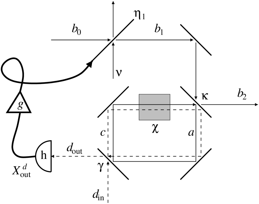
Figure 2: Diagram for a traveling-wave feedback experiment based on a QND measurement. Traveling fields are denoted $b$ and $d$. The first beam splitter transmittance $\eta_{1}$ is variable. A cavity (drawn as a ring cavity for convenience) supports two modes, $a$ (solid line) and $c$ (dashed line). The decay rates for these two modes are $\kappa$ and $\gamma$ respectively. They are coupled by a nonlinear optical process indicated by the crystal labeled $\chi$. The perfect homodyne detection at the detector labeled h yields a photocurrent proportional to $X^{d}_{\rm out}=d_{\rm out}+d_{\rm out}^{\dagger}$

Ignoring practicalities, I will take the coupling between the two modes to be the ideal QND coupling, as considered initially by Hillery and Scully [34] and Yurke [35], namely

$$H=\frac{\chi}{2}x^{a}y^{c},$$ (102)

where

$$x^{a}=a+a^{\dagger}\;;\;\;\;y^{c}=-ic+ic^{\dagger}.$$ (103)

As described in [36], this Hamiltonian could in principle be realized by a crystal with a $\chi^{(2)}$ nonlinearity, combined with other processes. This Hamiltonian commutes with the $x^{a}$ quadrature of mode $a$, and causes this to drive the $x^{c}$ quadrature of mode $c$. Thus measuring the $X^{d}_{\rm out}$ quadrature of the output field $d_{\rm out}$ from mode $c$ will give a QND measurement of $a+a^{\dagger}$, which is approximately a QND measurement of $X^{b}_{\rm in}$.

Following the analysis of [36], the quantum Langevin equations for the quadrature operators are

$$\dot{x}^{a} = -\frac{\kappa}{2}x^{a}-\sqrt{\kappa}\,X^{b}_{\rm in},$$ (104)

$$\dot{x}^{c} = -\frac{\gamma}{2}x^{c}-\sqrt{\gamma}\,X^{d}_{\rm in}+\chi x^{a}.$$ (105)

These can be solved in the frequency domain as

$$\tilde{x}^{a}(\omega) = -\frac{\sqrt{\kappa}\,\tilde{X}_{\rm in}^{b}(\omega)}{\kappa/2+i\omega}$$ (106)

$$\tilde{x}^{c}(\omega) = -\frac{\sqrt{\gamma}\,\tilde{X}_{\rm in}^{d}(\omega)+\sqrt{\kappa}\chi\tilde{X}_{\rm in}^{b}(\omega)/(\kappa/2+i\omega)}{\gamma/2+i\omega}.$$ (107)

The quadrature of the output field $d_{\rm out}=d_{\rm in}+\sqrt{\gamma}c$ is therefore

$$\tilde{X}^{d}_{\rm out}(\omega)=-\frac{\gamma\kappa Q\,\tilde{X}_{\rm in}^{b}(\omega)/(\kappa+2i\omega)+(\gamma-2i\omega)\tilde{X}_{\rm in}^{d}(\omega)}{\gamma+2i\omega},$$ (108)

where I have defined a quality factor for the measurement

$$Q=4\chi/\sqrt{\gamma\kappa}.$$ (109)

In the limits $\omega\ll\kappa,\gamma$ and $Q\gg 1$ we have

$$\tilde{X}^{d}_{\rm out}(\omega)\simeq-Q\tilde{X}_{\rm in}^{b}(\omega),$$ (110)

which shows that a measurement (by homodyne detection) of the $X$ quadrature of $d_{\rm out}$ does indeed effect a measurement of the low frequency variation in $X_{\rm in}^{b}$.

To see that this measurement is a QND measurement we have to calculate the statistics of the output field from mode $a$, that is $b_{\rm out}$. From the solution (106) we find

$$\tilde{X}^{b}_{\rm out}(\omega)=-\frac{\kappa/2-i\omega}{\kappa/2+i\omega}\tilde{X}^{b}_{\rm in}(\omega).$$ (111)

That is, apart from an irrelevant phase factor the output field is identical to the input field, as required for a QND measurement. Of course we cannot expect the other quadrature to remain unaffected, because of the uncertainty principle. Indeed we find

$$\tilde{Y}^{b}_{\rm out}(\omega)=-\frac{(\kappa-2i\omega)}{\kappa+2i\omega}\tilde{Y}_{\rm in}^{b}(\omega)+\frac{Q\gamma\kappa\,\tilde{Y}_{\rm in}^{d}(\omega)/(\gamma+2i\omega)}{\kappa+2i\omega},$$ (112)

which shows that noise has been added to $Y_{\rm in}$. Indeed, in the good measurement limit which gave the result (110) we find the phase quadrature output to be dominated by noise:

$$\tilde{Y}^{b}_{\rm out}(\omega)\simeq Q\tilde{Y}_{\rm in}^{d}(\omega).$$ (113)

5.2 QND-based Feedback

We know wish to show how a QND measurement, such as that just considered, can be used to produce squeezing via feedback. The physical details of how the feedback can be achieved are as outlined in Sec. 3.1 In particular, in the limit that the transmittance $\eta_{1}$ of the modulated beam splitter goes to unity, the effect of the modulation is simply to add an arbitrary signal to the amplitude quadrature of the controlled beam. That is, the modulated beam can be taken to be

$$b_{1}(t)=b_{0}(t-\tau_{1})+\beta\delta\eta_{1}(t-\tau_{1}),$$ (114)

where $b_{0}$ is the beam incident on the modulated beam splitter, as in Sec. 3.1. In the present case, $b_{1}(t)$ is then fed into the QND device, as shown in Fig. 2, so

$$b_{\rm in}(t)=b_{1}(t),$$ (115)

and the modulation is controlled by the photocurrent from a (assumed perfect) homodyne measurement of $X^{d}_{\rm out}$:

$$\delta\eta_{1}(t)=\frac{{g}}{-Q\beta}\int_{0}^{\infty}h(s)X^{d}_{\rm out}(t-\tau_{0}-s)ds.$$ (116)

Here $\tau_{0}$ is the delay time in the feedback loop, including the time of flight from the cavity for mode $c$ to the homodyne detector, and $h(s)$ is as before.

Substituting (114)-(116) into the results of the preceding subsection we find

$$\tilde{X}_{\rm out}^{b}(\omega)=-\frac{\kappa-2i\omega}{\kappa+2i\omega}\frac{\tilde{X}_{\rm in}^{b}(\omega)+\tilde{X}_{\rm in}^{d}(\omega){g}\tilde{h}(\omega)Q^{-1}\frac{\gamma-2i\omega}{\gamma+2i\omega}}{1-{g}\tilde{p}(\omega)\tilde{h}(\omega)\exp(-i\omega T)},$$ (117)

where $T=\tau_{1}+\tau_{0}$ is the total round-trip delay time, and

$$\tilde{p}(\omega)=\frac{\gamma\kappa}{(\kappa+2i\omega)(\gamma+2i\omega)}$$ (118)

represents the frequency response of the two cavities. If we assume that the field $d_{\rm in}$ is in the vacuum state then we can evaluate the spectrum of amplitude fluctuations in $X_{\rm out}^{b}$ to be

$$S_{\rm out}^{X}(\omega)=\frac{S_{\rm in}^{X}(\omega)+{g}^{2}Q^{-2}}{|1-{g}\tilde{p}(\omega)\tilde{h}(\omega)\exp(-i\omega T)|^{2}}.$$ (119)

Clearly in the limit $Q\to\infty$, the added noise term in the amplitude spectrum can be ignored. Then for sufficiently large negative ${g}$ the feedback will produce a sub-shot noise spectrum. Note the difference between this case and that of Sec. 3. Here the squeezed light is not part of the feedback loop; it is a free beam. The ultimate limit to how squeezed the beam can be is caused by the noise in the measurement. In the limit ${g}\to-\infty$ we find

$$S_{\rm out}^{X}(\omega)_{\rm min}=|Q\tilde{p}(\omega)\tilde{h}(\omega)|^{-2}.$$ (120)

Since $b_{\rm out}$ is a free field, not part of any feedback loop, it should obey the standard commutation relations. This is the case, as can be verified from the expression (112) for $Y_{\rm out}^{b}$ (which is unaffected by the feedback). Consequently, the spectrum for the phase quadrature

$$S_{\rm out}^{Y}(\omega)=S_{\rm in}^{Y}(\omega)+|Q\tilde{p}(\omega)|^{2}$$ (121)

shows the expected increase in noise. It is not difficult to show that the uncertainty product $S_{\rm out}^{Y}(\omega)S_{\rm out}^{X}(\omega)$ is greater than or equal to unity, as required.

5.3 Parametric Down Conversion

The preceding section showed that feedback based on a perfect QND measurement can produce squeezing. This has never been done experimentally because of the difficulty of building a perfect QND measurement apparatus. However, it turns out that QND measurements are not the only way to produce squeezing via feedback. Any mechanism which produces correlations between the beam of interest and another beam which are more “quantum” than the correlations between the two outputs of a linear beam splitter can be the basis for producing squeezing via feedback. Such a mechanism must involve some sort of optical nonlinearity, which is why this section V is entitled “Feedback based on Nonlinear Measurements”.

The production of amplitude squeezing by feeding back a quantum - correlated signal was predicted [37] and observed [38] by Walker and Jakeman in 1985, using the process of parametric down-conversion. An improved feedback scheme for the same system was later used by Tapster, Rarity and Satchell [39] to obtain an inferred amplitude spectrum $S_{1}^{X}(\omega)_{\rm min}=0.72$ over a limited frequency range.

The essential idea is as follows. A non-degenerate optical parametric oscillator (NDOPO) can be realized by pumping a crystal with a $\chi^{(2)}$ nonlinearity by a laser of frequency $\omega_{1}$ and momentum ${\bf k}_{1}$. For particular choices of $\omega_{1}$ the crystal can be aligned so that a pump photon can be transformed into a pair of photons each with frequencies $\omega_{2},\omega_{3}$ and momenta ${\bf k}_{2},{\bf k}_{3}$ with $\omega_{1}=\omega_{2}+\omega_{3}$ and ${\bf k}_{1}={\bf k}_{2}+{\bf k}_{3}$. A pair of down-converted photons will thus be correlated in time because they are produced from a single pump photon. On a more macroscopic level, this means that the amplitude quadrature fluctuations in the two down-converted beams are positively correlated, and the coefficient of correlation can in principle be very close to unity. In this ideal limit, measuring the intensity of beam 2 should give a readout identical to that obtained from measuring beam 3.In effect, the measurement of beam 2 is like a QND measurement of beam 3. Thus, feeding back the photocurrent from beam 2 with an negative gain should be able to reduce the noise in beam 3 below the shot-noise limit. In the limit of perfect detection, the optimum gain becomes arbitrarily large.

In  [37, 39] the negative feedback was effected by controlling the power of the pump laser (which controls the rate at which photon pairs are produced). This maintains the symmetry of the experiment so that the fed-back photocurrent from beam $2$ has the same statistics as the photocurrent from the free beam $3$. In other words, they will both be below the shot-noise, whereas without feedback they are both at best shot-noise limited. However, it is not necessary to preserve the symmetry in this way. The measured photocurrent from beam $2$ can be fed forward to control the amplitude fluctuations in beam $3$ (for example by using an electro-optic modulator as described in Sec. 3.1). This feedforward was realized experimentally by Mertz et al. in 1990 [40] achieving similar results to that obtained by feedback [41]. The lesson is that unless one is concerned with light inside a feedback loop, there is no essential difference between feedback and feedforward. Indeed, the squeezing produced by QND-based feedback discussed in Sec. 121 could equally well have been produced by QND-based feedforward.

5.4 Second Harmonic Generation

A third example of using quantum correlations between two beams to good effect in a feedback (or feedforward) loop is that of second-harmonic generation. Like parametric down conversion, this involves a $\chi^{(2)}$ crystal, but here the two low frequency modes are assumed to be degenerate, so that $\omega_{2}=\omega_{3}$ and ${\bf k}_{2}={\bf k}_{3}$, and the polarizations are the same also. For simplicity, I will call the low frequency mode the red mode and the high frequency mode with frequency $\omega_{1}=2\omega_{2}$ the green mode. For second harmonic generation, it is the red mode which is pumped (that is, the reverse of parametric down-conversion). In this case, the pumped mode (red) is also treated as a quantum system so that the two beams are the red and green beams. The system is easily treated using quantum Langevin equations [42].

The proposal made in [43] is as follows. The first harmonic (red) resides in a good cavity and is driven by a laser at the end with very high reflectivity. The second harmonic (green), which is generated in the red cavity, is reflected at one end only (giving two passes) so that it forms a single output beam. By itself (that is, in the absence of feedback) this system produces amplitude squeezing in both the first and second harmonic [44]. The amplitude squeezing in the red can be understood to be due to two-photon absorption, which is the effect of the adiabatically eliminated green mode. Such nonlinear absorption preferentially damps large fluctuations and so reduces the variance. The antibunching in the green mode can be attributed to the fact that the creation of a green photon requires the loss of two red photons, which reduces the chances of this event re-occurring.

Without feedback, the optimum low frequency squeezing in the red mode output is

$$S^{X}_{r}(0)=\frac{2}{3}\;\;\;{\rm for}\;\;\chi=\frac{1}{3},$$ (122)

and that in the green mode is

$$S_{g}^{X}(0)=\frac{1}{9}\;\;\;{\rm for}\;\;\chi\to\infty.$$ (123)

Here $\chi$ is the ratio of the nonlinear intensity loss rate to the linear intensity loss rate for the red mode. Now there are two possible ways to feed back onto the driving of the system. The first is to use the green photocurrent to control the amplitude of the red driving, in order to try to reduce the noise in the red output light. A linearized treatment gives a new minimum of

$$S^{X}_{r}(0)=\frac{1}{2}\;\;\;{\rm for}\;\;\chi=1,\;\;g=\frac{1}{2},$$ (124)

which is significantly less than the no-feedback value (122). Here, $g$ is the low frequency loop transfer function, equal to the round-loop gain of the feedback [28]. Note that it is positive, corresponding to destabilizing feedback. This is different from the cases of QND-based feedback and down-conversion-based feedback.

The other sort of feedback is to control the driving of the red mode using the detected red photocurrent, looking to enhance the squeezing in the green output. It turns out that the minimum $S_{g}^{X}(0)$ of (123) as $\chi\to\infty$ cannot be lowered by feedback. However, for finite values of $\chi$, the feedback can give a definite improvement. For example, with no feedback

$$S_{g}^{X}(0)=\frac{1}{2}\;\;\;{\rm for}\;\;\chi=1,$$ (125)

whereas the optimal feedback gives

$$S_{g}^{X}(0)=\frac{1}{3}\;\;\;{\rm for}\;\;\chi=1,\;\;g=\frac{1}{4}.$$ (126)

All of these results are calculated for the case of unit efficiency photodetectors. The effect of non-unit efficiency is to reduce the effectiveness of the feedback, and to alter the conditions of optimality. The general solution, including the full spectrum with an arbitrary transfer function $g\tilde{h}(\omega)$, is contained in [43].

6 Quantum Trajectories

6.1 The Master Equation

The Quantum Langevin Equation (QLE) considered in Sec. 4 are Heisenberg picture equations which detail the effect of the bath on the system. They also, through the input-output relations, specify the effect of the system on the bath, and hence the relation between the system evolution and the measured photocurrents. For systems which have linear QLEs, this is the easiest method to analyze their evolution. However, even some simple systems (such as a two-level atom) do not have linear QLEs. Also, sometimes a better intuition about feedback can be gained by working in the Schrödinger picture rather than the Heisenberg picture.

If one is interested only in the evolution of the system then there is a simple Schrödinger picture equivalent to the QLE. This is the quantum master equation, an example of which was already derived as (98) from the corresponding QLE. Unlike a QLE, a master equation is always a linear equation. It is possible to derive the master equation directly from the system-bath coupling without deriving the QLE, simply by tracing over the bath. I present this derivation below, because it shows clearly that this step (ignoring the bath) is not an essential one. If instead of ignoring the bath, one measures it, then one obtains a quantum trajectory equation. This is a different sort of Schrödinger picture equivalent to the QLE which is more general than the master equation, as it can also relate the system evolution to the measured photocurrents. This is necessary if one is to consider feeding back the photocurrent to alter the dynamics of the system.

For convenience, I will work in the interaction picture, rather than the Schrödinger picture, so that the free evolution causing the oscillation of the dipole can be ignored. The interaction between the system and the bath is now given by

$$V(t)={i}\hbar\sqrt{\gamma}\,[b^{\dagger}(t)c-c^{\dagger}b(t)],$$ (127)

where $c$ is a slowly-varying interaction picture operator, and $b(t)$ is also a slowly-varying interaction picture bath operator. The time-dependence is maintained for the bath operator, because the free Hamiltonian of the bath causes propagation at the speed of light, so a new part of the bath interacts with the system at each new point in time. These parts are labeled by the time of interaction $t$. Thus, $b(t)$ is an operator in the Hilbert space for a particular part of the bath. Each part has its own state matrix $\mu(t)$. For the incoming field to be a bath requires that its total state matrix be the direct product of the state matrices of the parts [14]. That is to say, the temporally separate parts of the bath must be unentangled.

Let the system at time $t$ be known to be $\rho(t)$. Thus the initial state of the system and (relevant part of the) bath at time $t$ is

$$R(t)=\mu(t)\otimes\rho(t).$$ (128)

The infinitesimally evolved state is

$$R(t+dt)=U(t,t+dt)[\mu(t)\otimes\rho(t)]U^{\dagger}(t,t+dt),$$ (129)

where

$$U(t,t+dt)=\exp\left[\sqrt{\gamma}\,dB^{\dagger}(t)c-c^{\dagger}\sqrt{\gamma}\,dB(t)-iHdt\right],$$ (130)

where $H$ is the system Hamiltonian in the interaction picture. If the input bath is in the vacuum state then all of the first and second order moments of $dB(t)$ vanish except, as in (94),

$${\rm Tr}[dB(t)dB^{\dagger}(t)\mu(t)]=dt.$$ (131)

Thus, it is necessary to expand some of the terms in $U(t,t+dt)$ to second order. The result for $R(t+dt)$ is

$$\mu(t)\otimes\rho(t)+\sqrt{\gamma}\,\left[dB^{\dagger}(t)c-c^{\dagger}dB(t),\mu(t)\otimes\rho(t)\right]$$ (132)

$$+\gamma\left\{dB^{\dagger}(t)\mu(t)dB(t)\otimes c\rho(t)c^{\dagger}-\mbox{$\frac{1}{2}$}dB(t)dB^{\dagger}(t)\mu(t)\otimes c^{\dagger}c\rho\right.$$

$$-\left.\mbox{$\frac{1}{2}$}\mu(t)dB(t)dB^{\dagger}(t)\otimes\rho c^{\dagger}c\right\}-i[Hdt,\mu(t)\otimes\rho(t)].$$

The infinitesimally evolved reduced state matrix for the system is given by

$$\rho(t+dt)={\rm Tr}_{\mu}[R(t+dt)].$$ (133)

Taking the trace over the bath state in (132) yields the master equation (98):

$$\dot{\rho}=\gamma{\cal D}[c]\rho-i[H,\rho].$$ (134)

The first term here represents irreversible evolution (damping in this case), and is of the unique form for such evolution as proved by Lindblad [45]. The second term represents unitary evolution which is of course reversible.

6.2 Photon Counting

To consider measuring the output bath it is useful to explicitly write down its state. Before interacting with the system, the input bath state is $\mu(t)=|{0}\rangle\langle{0}|$ for all time $t$, where $|{0}\rangle$ is the lowest eigenstate for $a^{\dagger}a$. Here, $a=\sqrt{dt}\,b_{0}(t)=dB_{0}(t)/\sqrt{dt}$, so that $a^{\dagger}a$ has integer eigenvalues representing the number of photons arriving in the interval of time $[t,t+dt)$. Let the state of the system at time $t$ be $\rho(t)$, independent of $\mu(t)$. The entangled state after the interaction of duration $dt$ is, from (132)

$$R(t+dt) = |{0}\rangle\langle{0}|\otimes\rho(t)+\sqrt{\gamma dt}\left[|{1}\rangle\langle{0}|\otimes c\rho(t)+|{0}\rangle\langle{1}|\otimes\rho(t)c^{\dagger}\right]$$ (135)

$$-{i}dt|{0}\rangle\langle{0}|\otimes[H,\rho(t)]+\;\gamma dt\left\{|{1}\rangle\langle{1}|\otimes c\rho(t)c^{\dagger}\right.$$

$$-\left.\mbox{$\frac{1}{2}$}|{0}\rangle\langle{0}|\otimes\left[c^{\dagger}c\rho(t)+\rho(t)c^{\dagger}c\right]\right\}.$$

The free dynamics of the electromagnetic field will now remove the bath state from the system, so that the entanglement in (135) will be maintained. If the outgoing bath is ignored, then the system obeys the master equation (134).

To obtain information about the system, the outgoing field must be measured. The obvious measurement to consider is photon counting. This I will model by projecting the field states onto eigenstates of $a^{\dagger}a$. It is possible to consider specific models for photon detectors, usually based on atomic systems [2]. However, these simply remove the measurement step, where possibilities become actualities, one step further along the von Neumann chain [46]. There is little which results from such models which cannot be achieved by including losses and convolving the classical photocurrent with an empirically derived detector response function. Therefore, I will simply use projection measurement operators

$$P_{0}=|{0}\rangle\langle{0}|\;;\;\;P_{1}=|{1}\rangle\langle{1}|.$$ (136)

If there is a null count then the unnormalized state matrix of the system and bath (whose norm gives the probability of this outcome) is given by

$$\tilde{R}_{0}(t+dt)=P_{0}R(t+dt)P_{0}=P_{0}\otimes\tilde{\rho}_{0}(t+dt),$$ (137)

where

$$\tilde{\rho}_{0}(t+dt)=\rho(t)-\gamma\mbox{$\frac{1}{2}$}\{c^{\dagger}c,\rho(t)\}dt-{i}[H,\rho(t)]dt.$$ (138)

This has a norm only infinitesimally different from one, so for almost all time intervals no photons are detected in the output.

If a photon is detected, then $\tilde{R}_{1}(t+dt)=P_{1}\otimes\tilde{\rho}_{1}(t+dt)$. That is, the system jumps into the unnormalized conditioned state

$$\tilde{\rho}_{1}(t+dt)=\gamma c\rho(t)c^{\dagger}dt.$$ (139)

The norm of this state matrix is equal to the probability of a detection occurring in the interval $[t,t+dt)$, and is equal to $\gamma\langle c^{\dagger}c\rangle dt$. Clearly, the unconditioned master equation evolution (134) is retrieved by averaging over the two possible results

$$\rho(t+dt)=\tilde{\rho}_{0}(t+dt)+\tilde{\rho}_{1}(t+dt).$$ (140)

It is useful and elegant to reformulate this evolution in the form of an explicitly stochastic evolution equation. This equation of motion specifies the quantum trajectory of the system. Since the measurement result is a point process, it can be represented by a random variable $dN_{\rm c}(t)$ representing the increment (either zero or one) in the photon count in the interval $[t,t+dt)$. It is formally defined by

$${\rm E}[dN_{\rm c}(t)] = {\rm Tr}[c^{\dagger}c\rho_{\rm c}(t)]\gamma dt,$$ (141)

$$dN_{\rm c}(t)^{2} = dN_{\rm c}(t).$$ (142)

Here the subscript ${\rm c}$ indicates that the quantity to which it is attached is conditioned on previous measurement results, arbitrarily far back in time. The conditioned state matrix obeys the stochastic master equation (SME)

$$d\rho_{\rm c}(t)=\left\{dN_{\rm c}(t){\cal G}[c]-dt{\cal H}\left[{i}H+\mbox{$\frac{1}{2}$}\gamma c^{\dagger}c\right]\right\}\rho_{\rm c}(t).$$ (143)

Here, the nonlinear (in $\rho$) superoperators ${\cal G}$ and ${\cal H}$ are defined by

$${\cal G}[r]\rho = \frac{r\rho r^{\dagger}}{{\rm Tr}[r\rho r^{\dagger}]}-\rho,$$ (144)

$${\cal H}[r]\rho = r\rho+\rho r^{\dagger}-{\rm Tr}[r\rho+\rho r^{\dagger}]\rho.$$ (145)

The nonlinearity of the SME (143) is indicative of the fundamental nonlinearity of quantum measurements. The original master equation for $\rho(t)={\rm E}[\rho_{\rm c}(t)]$ can be restored simply by replacing $dN_{\rm c}(t)$ in (143) by its ensemble average value (141).

Because of the assumed perfect detection, the stochastic equation for the state matrix is equivalent to a stochastic equation for the state vector. The unraveling of the master equation into a stochastic Schrödinger equation representing photon counting is the most commonly used quantum trajectory for numerical simulations [47, 48, 49, 50, 51, 52]. From the point of view of measurement theory, the stochastic master equation is of more use than the stochastic Schrödinger equation because it is more transparently related to the unconditioned master equation and because it can be generalized to cope with inefficient detectors. This will be dealt with explicitly for the case of homodyne detection.

6.3 Homodyne Detection Theory

The unraveling of the master equation (134) as a quantum trajectory is not unique. Different detection schemes will result in different quantum trajectory equations. For squeezing, the most useful detection technique is homodyne detection. In the simplest configuration, the output field of the cavity, $b_{\rm out}=\nu+\sqrt{\gamma}c$, is sent through a beam splitter of transmittance $\eta$ very close to one. Into the other input port of the beam splitter is injected a very strong coherent field. This has the same frequency as the system dipole, and is known as the local oscillator. The transmitted field is then represented by the operator

$$b_{1}=\nu+\sqrt{\gamma}c+\beta,$$ (146)

where $\beta$ is a complex number representing a coherent amplitude, such that $|\beta|^{2}/(1-\eta)$ is equal to the input photon flux of the local oscillator. The photodetection operators are then applied as above, with the annihilation operator defined as $a=b_{1}\sqrt{dt}$.

Let the coherent field $\beta$ be real, so that the homodyne detection leads to a measurement of the $x$ quadrature of the system dipole. Also, let us measure time in units of $\gamma^{-1}$ so that this parameter disappears from our equations. Then the rate of photodetections at the (perfect) detector

$${\rm E}[dN_{\rm c}(t)]={\rm Tr}[(\beta^{2}+\beta x+c^{\dagger}c)\rho_{\rm c}(t)]dt.$$ (147)

where $x=c+c^{\dagger}$ as previously. In the limit that $\beta$ is much larger than $c$, this rate consists of a large constant term plus a term proportional to $x$, plus a small term. It is not difficult to show that the SME for the conditioned state matrix is altered from (143) to

$$d\rho_{\rm c}(t)=\left\{dN_{\rm c}(t){\cal G}[c+\beta]+dt{\cal H}\left[-{i}H-\beta c-\mbox{$\frac{1}{2}$}c^{\dagger}c\right]\right\}\rho_{\rm c}(t).$$ (148)

The ideal limit of homodyne detection is when the local oscillator amplitude goes to infinity. In this limit, the rate of photodetections goes to infinity, but the effect of each on the system goes to zero, because the field being detected is almost entirely due to the local oscillator. Thus, it should be possible to approximate the photocurrent by a continuous function of time, and also to derive a smooth evolution equation for the system. This was done first by Carmichael [13]. A more rigorous working of the derivation is found in [53]. The result is that over a time much longer than $\beta^{-3/2}$, but much smaller than unity, the system evolution can be approximated by the SME

$$d\rho_{\rm c}(t)=-{i}[H,\rho_{\rm c}(t)]dt+{\cal D}[c]\rho_{\rm c}(t)dt+dW(t){\cal H}[c]\rho_{\rm c}(t).$$ (149)

Here $dW(t)$ is an infinitesimal Wiener increment [54] satisfying

$${\rm E}[dW(t)] = 0,$$ (150)

$$dW(t)^{2} = dt.$$ (151)

Thus, the jump evolution of (148) has been replaced by diffusive evolution. Equation (149) is, by its derivation, an Itô stochastic master equation, where the equal-time stochastic increment $dW(t)$ is independent of the state of the system $\rho_{\rm c}(t)$. It is trivial to see that the ensemble average evolution reproduces the nonselective master equation (134) by eliminating the noise term.

Just as the $\beta\to\infty$ leads to continuous evolution for the state, it also changes the point process photocount into a continuous photocurrent with white noise. Removing the constant local-oscillator contribution and scaling appropriately gives

$$I_{\rm c}^{\rm hom}(t)\equiv\lim_{\delta t\to 0}\lim_{\beta\to\infty}\frac{\delta N_{\rm c}(t)-\beta^{2}\delta t}{\beta\delta t}=\langle{x}\rangle_{\rm c}(t)+\xi(t),$$ (152)

where $\xi(t)=dW(t)/dt$. It is not difficult to see that if the detector efficiency is $\eta$, the homodyne photocurrent becomes

$$I_{\rm c}^{\rm hom}(t)\equiv\lim_{\delta t\to 0}\lim_{\beta\to\infty}\frac{\delta N_{\rm c}(t)-\eta\beta^{2}\delta t}{\sqrt{\eta}\,\beta\delta t}=\sqrt{\eta}\,\langle{x}\rangle_{\rm c}(t)+\xi(t),$$ (153)

and the SME (149) is modified to

$$d{\rho}=-{i}[H,\rho_{\rm c}(t)]dt+{\cal D}[c]\rho_{\rm c}(t)dt+\sqrt{\eta}dW(t){\cal H}[c]\rho_{\rm c}(t).$$ (154)

6.4 Homodyne-mediated Feedback

In the following section I will consider the use of feedback to produce or enhance squeezing in intracavity fields. Since squeezing is the reduction in fluctuations of one quadrature of a field, the obvious sort of feedback to consider is one using the homodyne photocurrent obtained from measuring the output field. Here I will develop the theory for describing this sort of feedback. As well as being more relevant for our purposes than feedback using the direct detection photocurrent [12], it is also somewhat easier to treat theoretically, which is why it was derived first [10, 11].

In principle, the homodyne photocurrent could be subject to any sort of filtering prior to being fed back, including nonlinear filtering. However it turns out that for the applications we wish to consider, only linear filtering is desired. Also, rather than using a response function $h(t)$ I will simply take the feedback to be delayed by a time $T$. That means that the evolution due to the feedback can simply be written as

$$[\dot{\rho}_{\rm c}(t)]_{\rm fb}=I_{\rm c}^{\rm hom}(t-T){\cal K}\rho_{\rm c}(t)/\sqrt{\eta},$$ (155)

where ${\cal K}$ is a superoperator. Since $I_{\rm c}^{\rm hom}(t)$ may be negative, ${\cal K}$ must be such as to give valid evolution irrespective of the sign of time. That is to say, it must give reversible evolution with

$${\cal K}\rho\equiv-{i}[F,\rho]$$ (156)

for some Hermitian operator $F$. In other words, we can represent the effect of the feedback by the Hamiltonian

$$H_{\rm fb}=F\left[\langle{c+c^{\dagger}}\rangle_{\rm c}(t-T)+\xi(t-T)/\sqrt{\eta}\right].$$ (157)

Because the stochasticity in the measurement (154) and the feedback (155) is Gaussian white noise, it is relatively simple to determine the effect of the feedback. Bearing in mind that the feedback must act after the measurement, and that (155) must be interpreted as a Stratonovich equation [11], the result for the total conditioned evolution of the system is

$$\rho_{\rm c}(t+dt) = \left\{1+{\cal K}[\langle c+c^{\dagger}\rangle_{\rm c}(t-T)dt+dW(t-T)/\sqrt{\eta}\,]+\frac{1}{2\eta}{\cal K}^{2}dt\right\}$$ (158)

$$\times\bigl{\{}1+{\cal H}[-{i}H]dt+{\cal D}[c]dt+\sqrt{\eta}dW(t){\cal H}[c]\bigr{\}}\rho_{\rm c}(t).$$

For $T$ finite, this becomes

$$d\rho_{\rm c}(t) = dt\left\{{\cal H}[-{i}H]+{\cal D}[c]+\langle{c+c^{\dagger}}\rangle_{\rm c}(t-T){\cal K}+\frac{1}{2\eta}{\cal K}^{2}\right\}\rho_{\rm c}(t)$$ (159)

$$+\,dW(t-T){\cal K}\rho_{\rm c}(t)/\sqrt{\eta}+\sqrt{\eta}dW(t){\cal H}[c]\rho_{\rm c}(t).$$

On the other hand, putting $T=0$ in (158) gives

$$d\rho_{\rm c}(t) = dt\left\{-{i}[H,\rho_{\rm c}(t)]+{\cal D}[c]\rho_{\rm c}(t)-{i}[F,c\rho_{\rm c}(t)+\rho_{\rm c}(t)c^{\dagger}]\right.$$ (160)

$$+\,\left.{\cal D}[F]\rho_{\rm c}(t)/\eta\right\}+dW(t){\cal H}[\sqrt{\eta}c-{i}F/\sqrt{\eta}\,]\rho_{\rm c}(t).$$

7 Intracavity Squeezing

7.1 The Linear System

In order to understand the effect of quantum limited feedback on intracavity squeezing, it is useful to consider an exactly solvable system. In this section, I will mainly be following [11] in considering the case of a linear optical system, with linear feedback based on homodyne (or QND) detection. By a linear system, I mean that the equation of motion for the two quadrature operators are linear. This is approximately the case for many quantum optical systems, in the limit of large photon numbers. For specificity, I will chose a system which is exactly linear. If, as in the remainder of this chapter, one is interested in the behaviour of one quadrature only (here the $x$ quadrature), then all linear dynamics can be composed of damping, driving, and parametric driving. Damping will be assumed to be always present (as necessary to do feedback or obtain an output from the cavity) and will have rate $1$. Constant linear driving simply shifts the origin away from $x=0$, and will be ignored. Stochastic linear driving in the white noise approximation causes diffusion in the $x$ quadrature, at a rate $l$. Finally, if the strength of the parametric driving ($H\sim xy$) is $\theta$ (where $\theta=1$ would represent a degenerate parametric oscillator at threshold), then the master equation for the system is

$$\dot{\rho}={\cal D}[a]\rho+\mbox{$\frac{1}{4}$}l{\cal D}[a^{\dagger}-a]\rho+\mbox{$\frac{1}{4}$}\theta[a^{2}-a^{\dagger}{}^{2},\rho]\equiv{\cal L}_{0}\rho,$$ (161)

where $a$ is the annihilation operator for the cavity mode.

An alternative definition for the linearity of the $x$ quadrature dynamics is that the marginal distribution of the Wigner function for $x$ (which is the true probability distribution for $x$) obeys an Ornstein-Uhlenbeck equation. That is to say,

$$\dot{P}(x)=\left(\partial_{x}kx+\mbox{$\frac{1}{2}$}D\partial_{x}^{2}\right)P(x),$$ (162)

where $k$ and $D$ are constants. The solution of this equation is a Gaussian with variance

$$V=\frac{D}{2k}.$$ (163)

For the particular master equation above (the properties of which will be denoted by the subscript $0$), the drift and diffusion constants are

$$k_{0} = \mbox{$\frac{1}{2}$}(1+\theta),$$ (164)

$$D_{0} = 1+l.$$ (165)

In this case, $V_{0}=(1+l)/(1+\theta)$. If this is less than unity, the system exhibits squeezing of $x$. It is more useful to work with the normally ordered variance, which becomes negative if the $x$ quadrature is squeezed. Here, I will denote it

$$U=V-1,$$ (166)

which for this system takes the value

$$U_{0}=\frac{l-\theta}{1+\theta}.$$ (167)

If the system is to stay below threshold (so that the $y$ quadrature does not become unbounded), then the maximum value for $\theta$ is one. At this value, $U_{0}=-1/2$ when the $x$ diffusion rate $l=0$. Therefore the minimum value of squeezing which this linear system can attain as a stationary value is half of the theoretical minimum of $U=-1$.

7.2 Homodyne-Mediated Feedback

We now wish to consider the effect of homodyne-mediated feedback on the intracavity light. This is most easily understood using the quantum trajectory picture in the Markovian limit. Thus we want the stochastic master equation for the conditioned state matrix $\rho_{\rm c}(t)$ (160)

$$d{\rho}_{\rm c}(t) = dt\left({\cal L}_{0}\rho_{\rm c}(t)+{\cal K}[a\rho_{\rm c}(t)+\rho_{\rm c}(t)a^{\dagger}]+\frac{1}{2\eta}{\cal K}^{2}\rho_{\rm c}(t)\right)$$ (168)

$$+\,dW(t)\left(\sqrt{\eta}{\cal H}[a]+{\cal K}/\sqrt{\eta}\right)\rho_{\rm c}(t).$$

Here, ${\cal L}_{0}$ is as defined in (161).

The question now arises as to what to choose for the ${\cal K}$. Seeking to reduce the fluctuations in $x$ suggests the feedback operator, which is related to ${\cal K}$ by (156), should be

$$F=-\lambda y/2.$$ (169)

As a separate Hamiltonian, this translates a state in the negative $x$ direction for $\lambda$ positive. By controlling this Hamiltonian by the homodyne photocurrent one thus has the ability to change the statistics for $x$ and perhaps achieve better squeezing. This Hamiltonian can be effected by driving the cavity (at a second mirror which can be assumed to have a negligible loss rate compared to the first mirror). Using this choice and changing (168) into a stochastic Liouville equation for the conditioned Wigner function gives

$$d{P}_{\rm c}(x) = dt\left[\partial_{x}(k_{0}+\lambda)x+\frac{1}{2}\partial_{x}^{2}\left(D_{0}+2\lambda+\lambda^{2}/\eta\right)\right]P_{\rm c}(x)$$ (170)

$$+\;dW(t)\left[\sqrt{\eta}\left(x-\bar{x}_{\rm c}(t)+\partial_{x}\right)+(\lambda/\sqrt{\eta})\partial_{x}\right]P_{\rm c}(x),$$

where $\bar{x}_{\rm c}(t)$ is the mean of the distribution $P_{\rm c}(x)$ and $dW(t)$ is as usual.

This equation is obviously no longer a simple Ornstein-Uhlenbeck equation. Nevertheless, it still has a Gaussian as an exact solution, as can be shown by direct substitution. The mean $\bar{x}_{\rm c}$ and variance $V_{\rm c}$ of the conditioned Gaussian distribution are found to obey

$$\dot{\bar{x}}_{\rm c} = -(k_{0}+\lambda)\bar{x}_{\rm c}+\xi(t)\left[\sqrt{\eta}\left(V_{\rm c}-1\right)-(\lambda/\sqrt{\eta})\right],$$ (171)

$$\dot{V}_{\rm c} = -2k_{0}V_{\rm c}+D_{0}-\eta\left(V_{\rm c}-1\right)^{2}.$$ (172)

Two points about the evolution equation for $V_{\rm c}$ are worth noting. It is completely deterministic (no noise terms), and it is not influenced by the presence of feedback. Furthermore, for this linear system, it is independent of $\bar{x}_{\rm c}$. Thus, the stochasticity and feedback terms in the equation for the mean do not even enter that for the variance indirectly.

The equation for the conditioned variance is more simply written in terms of the conditioned normally ordered variance $U_{\rm c}=V_{\rm c}-1$

$$\dot{U_{\rm c}}=-2k_{0}U_{\rm c}-2k_{0}+D_{0}-\eta U_{\rm c}^{2}.$$ (173)

On a time scale as short as a cavity lifetime, $U_{\rm c}$ will approach its stable steady-state value of

$$U_{\rm c}=\eta^{-1}\left(-k_{0}+\sqrt{k_{0}^{2}+\eta(-2k_{0}+D_{0})}.\right)$$ (174)

Substituting the steady-state conditioned variance into (171) gives

$$\dot{\bar{x}}_{\rm c}=-(k_{0}+\lambda)\bar{x}_{\rm c}+\xi(t)\frac{1}{\sqrt{\eta}}\left[-k_{0}+\sqrt{k_{0}^{2}+\eta(-2k_{0}+D_{0})}-\lambda\right].$$ (175)

If one were to choose

$$\lambda=-k_{0}+\sqrt{k_{0}^{2}+\eta(-2k_{0}+D_{0})}=-k_{0}+\sqrt{k_{0}^{2}+2\eta k_{0}U_{0}}$$ (176)

then there would be no noise at all in the conditioned mean and so one could set $\bar{x}_{\rm c}=0$. In other words, this value of $\lambda$ is precisely the value required to minimize the unconditioned variance under feedback. When all fluctuations in the mean are suppressed, the unconditioned variance is equal to the conditioned variance.

In general, the unconditioned variance will consist of two terms, the conditioned quantum variance in $x$ plus the classical (ensemble) average variance in the conditioned mean of $x$:

$$U_{\lambda}=U_{\rm c}+{\rm E}[\bar{x}_{\rm c}^{2}].$$ (177)

The latter term is found from (175) to be

$${\rm E}[\bar{x}_{\rm c}^{2}]=\eta^{-1}\frac{1}{2(k_{0}+\lambda)}\left[-(k_{0}+\lambda)+\sqrt{k_{0}^{2}+\eta(-2k_{0}+D_{0})}\right]^{2}.$$ (178)

Adding (174) gives

$$U_{\lambda}=\eta^{-1}\frac{\lambda^{2}+\eta(-2k_{0}+D_{0})}{2(k_{0}+\lambda)}=(k_{0}+\lambda)^{-1}\left(k_{0}U_{0}+\frac{\lambda^{2}}{2\eta}\right).$$ (179)

An immediate consequence of this expression is that $U_{\lambda}$ can only be negative if $U_{0}$ is. That is to say, classical feedback based on homodyne detection cannot produce intracavity squeezing. However, this does not mean that the feedback cannot enhance squeezing. Obviously, the best intracavity squeezing will be when $\eta=1$, in which case the intracavity squeezing can be simply expressed as

$$U_{\rm min}=k_{0}\left(-1+\sqrt{1+R_{0}}\right),$$ (180)

where $R_{0}=(-2k_{0}+D_{0})/k_{0}^{2}\geq-1$. It can be proven that that $U_{\rm min}\leq U_{0}$, with equality only if $\eta=0$ or $U_{0}=0$. This result implies that the intracavity variance in $x$ can always be reduced by classical homodyne-mediated feedback, unless it is at the classical minimum. In particular, intracavity squeezing can always be enhanced. For the parametric oscillator defined originally in (161), with $l=0$, $U_{\rm min}=-\theta/\eta$. For $\eta=1$, the (symmetrically ordered) $x$ variance is $V_{\rm min}=1-\theta$. The $y$ variance, which is unaffected by feedback, is seen from (161) to be $(1-\theta)^{-1}$. Thus, with perfect detection, it is possible to produce a minimum uncertainty squeezed state with arbitrarily high squeezing as $\theta\rightarrow 1$. This is not unexpected as a parametric amplifier (in an undamped cavity) also produces minimum uncertainty squeezed states. The feedback removes the noise which was added by the damping which is necessary to do the measurement used in the feedback.

The reason that this feedback cannot produce squeezing is that the conditioning of the variance according to (173) cannot change the sign of the normally-ordered variance $U$. The homodyne measurement does reduces the conditioned variance, except when it is equal to the classical minimum of 1. The more efficient the measurement, the greater the reduction. Ordinarily, this reduced variance is not evident because the measurement gives a random shift to the conditional mean of $x$, with the randomness arising from the shot noise of the photocurrent. By appropriately feeding back this photocurrent, it is possible to precisely counteract this shift and thus observe the conditioned variance.

If the time delay $T$ in the feedback loop is not negligible then the counteraction will be less than perfect. It is possible to calculate this effect exactly for an arbitrary linear feedback response using the quantum trajectory theory [11]. However, it would generally be easier to return to the approach based on quantum Langevin equations [55]. For short delay $T\ll 1$, there is a simple expression for the modified normally ordered variance:

$$U_{\lambda;T}=U_{\lambda}(1+\lambda T).$$ (181)

For squeezed systems, with $U_{0}<0$, the optimum value of $U_{\lambda}$ occurs for $\lambda$ negative, as shown above. Thus, the time delay reduces the total squeezing by the factor $(1+\lambda T)$. On the other hand, classical noise is reduced to $U_{\lambda}>0$ with $\lambda$ positive, so that the total noise is increased by the factor $(1+\lambda T)$. Overall, the time delay degrades the effectiveness of the feedback, as expected.

Note that the optimal $\lambda$ of (176) has the same sign as $U_{0}$. That is to say, if the system produces squeezed light, then the best way to enhance the squeezing is to add a force which displaces the state in the direction of the difference between the measured photocurrent and the desired mean photocurrent. This is the opposite of what would be expected classically, and can be attributed to the effect of homodyne measurement on squeezed states. For classical statistics ($U\geq 0$) , a higher than average photocurrent reading [$\xi(t)>0$] leads to the conditioned mean $\bar{x}_{\rm c}$ increasing (except if $U=0$ in which case the measurement has no effect). However, for nonclassical states with $U<0$, the classical intuition fails as a positive photocurrent fluctuation causes $\bar{x}_{\rm c}$ to decrease. This explains the counterintuitive negative value of $\lambda$ required in squeezed systems, which naively would be thought to destabilize the system and increase fluctuations. The value of the positive feedback required (176) is such that the overall restoring force $k_{0}+\lambda$ is still positive.

Succinctly, one can state that conditioning can be made practical by feedback. The intracavity noise reduction produced by classical feedback can be precisely as good as that produced by conditioning. This reinforces the simple explanation as to why homodyne-mediated classical feedback cannot produce nonclassical states: because homodyne detection cannot. Nonclassical feedback (such as using the photocurrent to influence nonlinear intracavity elements) may produce nonclassical states, but such elements can produce nonclassical states without feedback, so this is hardly surprising. In order to produce nonclassical states by classical feedback, it would be necessary to have a nonclassical measurement scheme. That is to say, one which does not rely on measurement of the extracavity light to procure information about the intracavity state. Intracavity measurements (in particular, quantum non-demolition measurements) are not limited by the random process of damping to the external continuum. The extra term which the measurement introduces into the nonselective master equation will not produce nonclassical states, but may allow the measurement to produce nonclassical conditioned states. One would thus expect that intracavity QND measurements would enable feedback to overcomes the classical limit, and I will now show that this is indeed the case.

7.3 QND-Mediated Feedback

The natural choice of quantum non-demolition variable is the quadrature to be squeezed, say $x$ as before. I use the same model for a QND measurement as in Sec. 5.1. Mode $a$ is coupled to mode $c$ by the Hamiltonian in (102). The other dynamics of mode $a$ are defined as before by its Liouville superoperator ${\cal L}_{0}$. The density operator for both modes thus obeys the following master equation:

$$\dot{R}={\cal L}_{0}R-\frac{\chi}{2}[x(c-c^{\dagger}),R]+\gamma{\cal D}[c]R.$$ (182)

In order to treat mode $c$ as part of the apparatus rather than part of the system, it is necessary to eliminate its dynamics. This can be done by assuming that it is heavily damped, with $\gamma$ much larger than all other rates. Then, apart from initial transients, it will have few photons and will be slaved to mode $a$. Following standard techniques for adiabatic elimination [53] gives the master equation for $\rho$, the density operator for mode $a$ alone, as

$$\dot{\rho}={\cal L}_{0}\rho+\Gamma{\cal D}[x/2]\rho,$$ (183)

where the measurement strength parameter is $\Gamma=4\chi^{2}/\gamma.$

Now add homodyne measurement of the $b$ mode with efficiency $\eta$. Starting from the conditioned state matrix $R_{\rm c}$ before the adiabatic elimination and following it through gives the conditioning master equation for $\rho_{\rm c}$ [11]

$$d{\rho}_{\rm c}=dt{\cal L}_{0}\rho_{\rm c}+dt\Gamma{\cal D}[x/2]\rho_{\rm c}+\sqrt{\rm\eta\Gamma}dW(t){\cal H}[x/2]\rho_{\rm c}.$$ (184)

Normalizing the homodyne photocurrent so that the noise is the same as in preceding sections gives

$$I_{\rm c}(t)=\sqrt{\rm H}\langle{x}\rangle_{\rm c}(t)+\xi(t).$$ (185)

Here I am using H (a capital $\eta$) for $\eta\Gamma$ as the effective efficiency of the measurement. This is related to the parameter $Q$ in Sec. 5.1 by ${\rm H}=\eta Q^{2}/4$. Note that this is not bounded above by unity, since it is possible for $\chi^{2}/\gamma$ to be much greater than one even with $\chi$ much less than $\gamma$. Recall that all rates are measured in units of the $a$ mode linewidth (which was $\kappa$ in Sec. 5.1).

The photocurrent (185) can be used in feedback onto the $a$ mode just as in preceding sections. A feedback term of the form

$$[\dot{\rho}_{\rm c}]_{\rm fb}=I_{\rm c}(t-T){\cal K}\rho_{\rm c}/\sqrt{\rm H}$$ (186)

gives, in the limit $T\rightarrow 0$, the conditioned evolution

$$d{\rho}_{\rm c} = dt\left({\cal L}_{0}\rho_{\rm c}+\Gamma{\cal D}[x/2]\rho_{\rm c}+{\cal K}\mbox{$\frac{1}{2}$}[x\rho_{\rm c}+\rho_{\rm c}x]+\frac{1}{2{\rm H}}{\cal K}^{2}\rho_{\rm c}\right)$$ (187)

$$+\;dW(t)\left(\sqrt{\rm H}{\cal H}[x/2]+{\cal K}/\sqrt{\rm H}\right)\rho_{\rm c}.$$

Using the same expressions as in Sec. 7.2 implies that the probability distribution for the $x$ quadrature obeys

$$d{P}_{\rm c}(x) = dt\left[\partial_{x}(k_{0}+\lambda)x+\frac{1}{2}\partial_{x}^{2}\left(D_{0}+\lambda^{2}/{\rm H}\right)\right]P_{\rm c}(x)$$ (188)

$$+\;dW(t)\left[\sqrt{\rm H}[x-\bar{x}_{\rm c}(t)]+(\lambda/\sqrt{H})\partial_{x}\right]P_{\rm c}(x).$$

The mean and variance of this conditioned distribution obey

$$\dot{\bar{x}}_{\rm c} = -(k_{0}+\lambda)\bar{x}_{\rm c}+\xi(t)\left(\sqrt{\rm H}V_{\rm c}-\lambda/\sqrt{\rm H}\right),$$ (189)

$$\dot{V}_{\rm c} = -2k_{0}V_{\rm c}+D_{0}-{\rm H}V_{\rm c}^{2}.$$ (190)

These equations are identical to the corresponding equations for homodyne mediated feedback (171) and (172) apart from the replacement of $(V_{\rm c}-1)$ by $V_{\rm c}$ and $\eta$ by ${\rm H}$ in the measurement terms. In the limit ${\rm H}\rightarrow\infty$, (190) predicts an arbitrarily small steady-state conditioned variance. This is characteristic of a good QND measurement. Of course, the quantum noise has not been eliminated but rather redistributed. For ${\rm H}$ to be large requires $\Gamma$ to be large also, so that the variance in the unsqueezed quadrature is greatly increased by the measurement term in (183). This ensures that Heisenberg’s uncertainty principle is not violated.

For this QND measurement the stationary value for $V$ from (190) is

$$V_{\rm c}={\rm H}^{-1}\left(-k_{0}+\sqrt{k_{0}^{2}+{\rm H}D_{0}}\right).$$ (191)

Thus choosing the feedback strength to be

$$\lambda=-k_{0}+\sqrt{k_{0}^{2}+{\rm H}D_{0}}.$$ (192)

eliminates the stochastic element in (189). In this case, the stationary conditioned variance (191) is the minimum achievable variance. In the limit ${\rm H}\rightarrow\infty$, it is easy to see that $V_{\rm min}=V_{\rm c}$ approaches the theoretical minimum value of $0$. That is, perfect squeezing can be produced inside the cavity by QND mediated feedback. In this limit, one requires the feedback to be very strong, with $\lambda\simeq\sqrt{{\rm H}D_{0}}$. Unlike the homodyne mediated feedback case, $\lambda$ should always be positive, as in accord with classical intuition. Indeed, all of the features of QND mediated feedback conform to a classical theory of feedback with measurements of finite accuracy (related to ${\rm H}$). The quantum nature of the feedback is manifest only in the increased fluctuations in $y$ due to the measurement back-action not present classically.

7.4 Mimicking a Squeezed Bath

The application of feedback based on a QND homodyne measurement to a cavity state has also been considered by Tombesi and Vitali [56]. However, rather than directly trying to minimize the $x$ quadrature variance of the field mode, as I have discussed above, their goal was to mimic the dynamics produced by shining a broad-band squeezed vacuum onto the cavity mirror. Being broad-band compared to the cavity mode, a squeezed vacuum input is parametrized by two numbers, $N,M$ which change the single nonzero second-order moments of (94) to

$$dB_{\rm in}^{\dagger}dB_{\rm in} = Ndt\;;\;\;dB_{\rm in}dB_{\rm in}^{\dagger}=(N+1)dt\;;\;\;$$

$$dB_{\rm in}dB_{\rm in} = (dB_{\rm in}^{\dagger}dB_{\rm in}^{\dagger})^{*}=Mdt.$$ (193)

Positivity of the bath state matrix requires $|M|^{2}\leq N(N+1)$ [2]. The master equation resulting from such bath correlations is [2]

$$\dot{\rho} = -i[H,\rho]+(N+1){\cal D}[a]+N{\cal D}[a^{\dagger}]$$ (194)

$$-M\mbox{$\frac{1}{2}$}[a^{\dagger},[a^{\dagger},\rho]]-M^{*}\mbox{$\frac{1}{2}$}[a,[a,\rho]].$$

Tombesi and Vitali show that an equation of this form can be produced using feedback based on a QND homodyne measurement and that, not surprisingly, it can can produce intracavity squeezing.

7.5 The Micromaser

A final example of feedback onto an intracavity state which can give nonclassical noise reduction is that of the micromaser [57]. This consists of a small microwave cavity through which a monochromatic beam of resonant two-level atoms is passed. The atomic state upon exit can be measured and the result used in feedback. The case of modifying the cavity quality factor has been considered by Liebman and Milburn [58]. Because of the nature of the Jaynes-Cummings Hamiltonian, the micromaser dynamics are complicated without feedback, and even more complicated with. However, one result is easy to explain. In the limit of short transit time the atoms (assumed all to enter in the upper state) act simply as a linear amplifier of the cavity mode. In the absence of feedback the stationary state is thermal, with a photon number variance much greater than the mean. With weak feedback, increasing the cavity damping rate whenever an outgoing atom is detected in the lower state, the photon distribution can be made sub-Poissonian, with a variance equal to half the mean. For longer transit times, the no-feedback dynamics show the effects of trapping states (where the atom undergoes an integer number of Rabi cycles in transit [57]), and the minimum stationary variance is typically as low as one quarter of the mean. Feedback can produce an arbitrary small minimum variance near a trapping state. However, this result is very sensitive to the transit time and so may be washed out by a realistic atomic velocity profile.

8 Feedback Master Equation

In (160) we have the stochastic master equation for a system undergoing homodyne measurement, with instantaneous linear feedback of the homodyne photocurrent. This is a Markovian Itô stochastic equation, so that is possible to take the ensemble average simply by removing the stochastic term. This removes all nonlinear terms from the stochastic master equation, and gives the deterministic master equation

$$\dot{\rho}=-{i}[H,\rho]+{\cal D}[c]\rho-{i}[F,c\rho+\rho c^{\dagger}]+\frac{1}{\eta}{\cal D}[F]\rho.$$ (195)

I will call this the homodyne feedback master equation. The first feedback term, linear in $F$, is the desired effect of the feedback which would dominate in the classical regime. The second feedback term causes diffusion in the variable conjugate to $F$. It can be attributed to the inevitable introduction of noise by the measurement step in the quantum-limited feedback loop. The lower the efficiency, the more noise introduced.

The homodyne feedback master equation can be rewritten in the Lindblad form [45] as

$$\dot{\rho}=-{i}\left[H+\mbox{$\frac{1}{2}$}(c^{\dagger}F+Fc),\rho\right]+{\cal D}[c-{i}F]\rho+\frac{1-\eta}{\eta}{\cal D}[F]\rho\equiv{\cal L}\rho.$$ (196)

In this arrangement, the effect of the feedback is seen to replace $c$ by $c-{i}F$, and to add an extra term to the Hamiltonian, plus an extra diffusion term which vanishes for perfect detection. It is possible to derive an analogous feedback master equation for direct detection, but this is not needed for squeezing. In the limit where intensity fluctuations can be linearized as amplitude quadrature fluctuations, direct detection is essentially equivalent to homodyne detection of the amplitude quadrature.

It is very important to note that although (196) has the appearance of a normal master equation, one cannot simply use it in the customary way for calculating the spectrum of the photocurrent used in the feedback loop. For example the two-time correlation function of the in-loop photocurrent is not given by the standard expression:

$${\rm E}[I_{\rm c}^{\rm hom}(t+\tau)I_{\rm c}^{\rm hom}(t)]\neq\eta\langle{:x(t+\tau)x(t):}\rangle+\delta(\tau),$$ (197)

where the normally ordered two-time correlation function for $x$ is defined as

$$\langle{:x(t+\tau)x(t):}\rangle={\rm Tr}\left\{(c+c^{\dagger})e^{{\cal L}\tau}[c\rho(t)+\rho(t)c^{\dagger}]\right\}.$$ (198)

That is because the photocurrent at time $t$ changes the system through the feedback as well as through the conditioning. Taking this into account, it is not difficult to show [12] that the correct expression is

$${\rm E}[I_{\rm c}^{\rm hom}(t+\tau)I_{\rm c}^{\rm hom}(t)] = \eta{\rm Tr}\left\{(c+c^{\dagger})e^{{\cal L}\tau}[(c-{i}F/\eta)\rho(t)\right.$$ (199)

$$+ \left.\rho(t)(c^{\dagger}+{i}F/\eta)]\right\}+\delta(\tau).$$

Note that the feedback is present in both the term in square brackets and the evolution by ${\cal L}$ for the time $\tau$. The former presence means that the in-loop photocurrent may have a sub-shot-noise spectrum, even if the system dynamics are classical. That is to say, for an optical system it may be possible to use an a semiclassical analysis (with classical light fields and detector shot noise) which nevertheless correctly predicts a sub-shot noise photocurrent spectrum. This is not surprising given the analogous result for free squeezing in Sec. 3.5.

9 In-loop Squeezing Revisited

9.1 In-Loop Squeezing

In Sec. 3 it was shown that a sub-shot-noise in-loop photocurrent is not evidence for squeezing of the in-loop light in the usual sense, not least because the usual two-time commutation relations do not apply to an in-loop field. Also, a linear optical element (a beam splitter) fails to extract any squeezing from the loop, and in fact produces an above-shot-noise output. Nevertheless it was also shown that an in-loop nonlinear optical element (a QND intensity meter) agrees with the intensity statistics seen by the in-loop detector. This means that it is an open question as to whether the effect of the in-loop “squashed” [31] light on other nonlinear optical elements is more akin to that of squeezed light or light with classical fluctuations.

The simplest nonlinear optical element is a two-level atom. Shortly after the first observation of squeezing, Gardiner [59] made a seminal prediction regarding its effects on such an atom [60], namely that immersing an atom in broad-band squeezed light would break the equality between the transverse decay rates for the two quadratures of the atomic dipole. In particular, one decay rate could be made arbitrarily small, producing an arbitrarily narrow line in the power spectrum of the atom’s fluorescence. This was seen, as the title of [59] proclaims, as a “direct effect of squeezing”.

In this section I present work published recently [61], which considers the question of whether this atomic line-narrowing is characteristic only of squeezing in the conventional sense (‘real squeezing’), or whether it can be produced by light which gives rise to a below shot-noise photocurrent by virtue of being part of a feedback loop (‘in-loop squeezing’). The answer is that in-loop squeezing can do the job. In fact, the inhibition of the decay of one quadrature depends on the amount of squeezing and the quality of mode-matching to the atom in exactly the same way for in-loop squeezing as for free-field squeezing. Thus in-loop squeezing appears likely to be an important tool for future experimental investigation of the effect of low-noise light on atoms, as it is usually easier to generate than free squeezing.

Consider the apparatus shown in Fig. 3, but for the moment without the fluorescent atom.

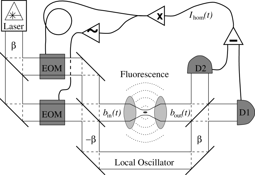
Figure 3: Diagram of the experimental configuration discussed in the text. All beam splitters are 50:50. The atom is represented by the small ellipse at the focus of $b_{\rm in}(t)$. The difference $I_{\rm hom}(t)$ between the photocurrents at detectors D1 and D2 is amplified and split. The two signals (with opposite sign) are fed back to the two electro-optic modulators (EOM)

The Mach-Zehnder interferometer on the left hand side has two functions. First it produces a weak beam ($b_{\rm in}$) which is given by

$$b_{\rm in}(t)=\nu(t)-(i/2)(\beta e^{i\phi}-\beta e^{-i\phi})\approx\nu(t)+\beta\phi.$$ (200)

Here $\beta$, assumed real, is the coherent amplitude of the laser, and $\pm\phi$, assumed small, are the phase shifts imposed by the electro-optic modulators. The operator $\nu(t)$ represents vacuum fluctuations as in Sec. 3. The second function of the interferometer is to produce a local oscillator beam with mean amplitude

$$-(1/2)(\beta e^{i\phi}+\beta e^{-i\phi})=-\beta[1+O(\phi^{2})].$$ (201)

With appropriate phase shifts assumed, this local oscillator is then used for making a homodyne measurement of the $X=b+b^{\dagger}$ quadrature of $b_{\rm out}$ (which, in the absence of the atom, is identical with $b_{\rm in}$). If the efficiency of the detectors is $\varepsilon$ then the homodyne photocurrent is represented by the operator [2]

$$I_{\rm hom}(t)=\sqrt{\varepsilon}\,X_{\rm out}(t)+\sqrt{1-\varepsilon}\,\xi_{\varepsilon}(t),$$ (202)

where $\xi_{\varepsilon}(t)$ is a unit-norm real white noise process.

Although $S^{X}_{\rm out}(\omega)$ is shot-noise limited for high frequencies, it need not be for lower frequencies. In particular, the feedback loop shown can produce a spectrum below the shot-noise as shown in Sec. 3. The current $I_{\rm hom}(t)$ is amplified and used to control $\phi$. If we set

$$\phi(t)=\frac{g}{2\beta\sqrt{\varepsilon}}\int_{0}^{\tau}h(t^{\prime})I_{\rm hom}(t-T-t^{\prime})dt^{\prime},$$ (203)

then we have a feedback loop with a low-frequency round-loop gain of $g$ which is stable under the conditions given in Sec. 3.2. Solving in the Fourier domain,

$$\tilde{X}_{\rm out}(\omega)=\left[{\tilde{\xi}_{\nu}(\omega)+g\tilde{h}(\omega)e^{-i\omega T}\sqrt{\frac{1-\varepsilon}{\varepsilon}}\,\tilde{\xi_{\varepsilon}}(\omega)}\right]\frac{1}{1-g\tilde{h}(\omega)e^{-i\omega T}}.$$ (204)

Thus $X_{\rm in}$ (which here equals $X_{\rm out}$) has a spectrum

$$S^{X}_{\rm in}(\omega)=[{1+g^{2}|\tilde{h}(\omega)|^{2}(\varepsilon^{-1}-1)}]/{|1-g\tilde{h}(\omega)e^{-i\omega T}|^{2}}.$$ (205)

At a frequency $\bar{\omega}$ much less than the feedback bandwidth $\sim\tau^{-1}$, and much less than the reciprocal of the delay time $T^{-1}$, $\tilde{h}(\bar{\omega})e^{-i\omega T}\simeq 1$ and the minimum noise is

$$S^{X}_{\rm in}(\bar{\omega})_{\rm min}=1-\varepsilon\;,\;\;{\rm for}\;g=-\varepsilon/(1-\varepsilon),$$ (206)

which is clearly below the standard quantum limit. These results reproduces those of (83), where here $\varepsilon$ is playing the same role as $\eta_{2}$.

9.2 An In-Loop Atom

Returning to Fig. 3, we now include the two-level atom, which is assumed to be resonant to the laser. It couples strongly only to modes of the radiation field having the appropriate dipole spatial distribution [1]. However, by focusing a beam as shown in Fig. 3, it is possible to mode-match a significant proportion, say $\eta$, of $b_{\rm in}$ into the atom’s input. Recent numerical calculations indicate that practical schemes for focusing light in free space have a limit on $\eta$ of order $0.1$ [62]. This suggests that in practice, a more efficient way to increase the effective $\eta$ would be to couple the light into a microcavity, as in [63]. However, it is conceptually simpler to consider the free-space set up in Fig. 3.

The Hamiltonian of the atom in the interaction picture at time $t$ is

$$H(t)=-i[\sqrt{\eta}\,b_{\rm in}(t)+\sqrt{1-\eta}\,\mu(t)]\sigma^{\dagger}(t)+{\rm H.c.}$$ (207)

Here $\sigma=|{g}\rangle\langle{e}|$ is the atomic lowering operator and I have set the longitudinal atomic decay rate to unity. The operator $\mu(t)$ represents an independent vacuum input. Under this coupling, the output field is found from the techniques of Sec. 4 to be

$$b_{\rm out}(t)=b_{\rm in}(t)+\sqrt{\eta}\,\sigma(t).$$ (208)

Although it would be possible to give a description of the entire feedback loop in terms of atomic and radiation field operators [61], it is simpler to use the quantum trajectory theory of homodyne measurement as outlined in Sec. 6. In this theory, only the atom is treated as a quantum mechanical system with state matrix $\rho(t)$; the rest of the apparatus is considered as a complicated measurement and feedback device for the atom. The photocurrent $I_{\rm c}^{\rm hom}(t)$ is therefore a classical quantity. From (153) it is given by

$$I_{\rm c}^{\rm hom}(t)=\bar{I}_{\rm c}^{\rm hom}(t)+\xi^{\rm hom}(t),$$ (209)

where $\xi^{\rm hom}(t)$ is local-oscillator shot noise, which in this case is the only source of noise in the whole system. From (202) and (208), the expected value $\bar{I}_{\rm c}^{\rm hom}(t)$ conditioned upon the prior photocurrent record is

$$\bar{I}_{\rm c}^{\rm hom}(t)=\sqrt{\eta\varepsilon}\,{\rm Tr}[\rho_{\rm c}(t)\sigma_{x}]+\sqrt{\varepsilon}\,2\beta\phi_{\rm c}(t).$$ (210)

Here $\phi_{\rm c}(t)$ is not set to its average value of zero because it is determined by the prior classical photocurrent via (203).

From the theory of Sec. 6, the atom will obey the following nonlinear stochastic master equation

$$d\rho_{\rm c}=dt{\cal D}[\sigma]\rho_{\rm c}+\sqrt{\eta\varepsilon}\,dW^{\rm hom}(t){\cal H}[\sigma]\rho_{\rm c}-idt[H_{\rm fb},\rho_{\rm c}].$$ (211)

The final Hamiltonian is due to the feedback. It is identical to the term due to feedback in the fundamental atomic Hamiltonian (207), namely

$$H_{\rm fb}(t)=\sqrt{\eta}\,\beta\phi(t)\sigma_{y}.$$ (212)

So far, it is not a singular quantity because of the smoothing of the photocurrent in (203).

Now consider the limit of instantaneous feedback on the atomic time-scale, $\tau,T\ll 1$. In this limit

$$2\beta\phi(t)=gI_{\rm c}^{\rm hom}(t)/\sqrt{\varepsilon}$$ (213)

and thus we can derive

$$I_{\rm c}^{\rm hom}(t)=(1-g)^{-1}\{\xi(t)+\sqrt{\eta\varepsilon}\,{\rm Tr}[\rho_{\rm c}(t)\sigma_{x}]\}.$$ (214)

Hence from (212) and (213),

$$H_{\rm fb}(t)=\lambda\mbox{$\frac{1}{2}$}\sigma_{y}\{{\rm Tr}[\rho_{\rm c}(t)\sigma_{x}]+\xi(t)/\sqrt{\eta\varepsilon}\,\},$$ (215)

where it is to be understood that $t$ on the right-hand side of this equation actually stands for $t-0^{+}$. Since $-\infty<g<1$, the feedback parameter $\lambda$ is given by

$$\lambda={g\eta}/({1-g})\;\in(-\eta,\infty).$$ (216)

Taking the Markovian limit allows us to derive a deterministic master equation for the atom. Equation (211) no longer applies, because $H_{\rm fb}(t)$ in (215) is singular. However, by comparison of (215) with (157) we see that we can follow the methods of Sec. 6.4 and Sec 8 to obtain

$$\dot{\rho}={\cal D}[\sigma]\rho-i\lambda[\mbox{$\frac{1}{2}$}\sigma_{y},\sigma\rho+\rho\sigma^{\dagger}]+\frac{\lambda^{2}}{\eta\varepsilon}{\cal D}[\mbox{$\frac{1}{2}$}\sigma_{y}]\rho.$$ (217)

This equation, and the following relation between $\lambda$ and the in-loop squeezing

$$S^{X}_{\rm in}(\bar{\omega})=\frac{1+g^{2}(\varepsilon^{-1}-1)}{(1-g)^{2}}=1+\frac{2\lambda}{\eta}+\frac{\lambda^{2}}{\eta^{2}\varepsilon},$$ (218)

are the central results of this section. In (218), we still have $\bar{\omega}\ll\tau^{-1}$, but now also $\bar{\omega}\gg 1$. This ensures that the atomic variables (with characteristic time scale of unity) do not contribute significantly to the spectrum at $\bar{\omega}$, so that (205) is still valid.

From the master equation (217) it is easy to derive the following dynamical equations:

$${\rm Tr}[\dot{\rho}\sigma_{x}] = -\gamma_{x}{\rm Tr}[\rho\sigma_{x}]$$ (219)

$${\rm Tr}[\dot{\rho}\sigma_{y}] = -\gamma_{y}{\rm Tr}[\rho\sigma_{y}]$$ (220)

$${\rm Tr}[\dot{\rho}\sigma_{z}] = -\gamma_{z}{\rm Tr}[\rho\sigma_{z}]-C$$ (221)

Only the equation for $\sigma_{y}$ is unaffected by the feedback, with $\gamma_{y}=1/2.$ The new decay rate for $\sigma_{x}$ is

$$\gamma_{x}=\frac{1}{2}\left[1+2\lambda+\frac{\lambda^{2}}{\eta\varepsilon}\right],$$ (222)

and the modified parameters for $\sigma_{z}$ are

$$\gamma_{z}=\gamma_{y}+\gamma_{x}\;,\;\;C=1+\lambda.$$ (223)

In steady state

$${\rm Tr}[\rho_{\rm ss}\sigma_{x}] = {\rm Tr}[\rho_{\rm ss}\sigma_{y}]=0,$$ (224)

$${\rm Tr}[\rho_{\rm ss}\sigma_{z}] = -1+{\lambda^{2}}/[{2\eta\varepsilon(1+\lambda)+\lambda^{2}}].$$ (225)

The most interesting of these results is that negative feedback can reduce the decay rate of the $x$ component of the atomic dipole below its natural value of $1/2$. From (218) it can be re-expressed as

$$\gamma_{x}=\mbox{$\frac{1}{2}$}\left[(1-\eta)+\eta S^{X}_{\rm in}(\bar{\omega})\right].$$ (226)

This clearly shows that $\gamma_{x}$ has two contributions: $\mbox{$\frac{1}{2}$}(1-\eta)$ from the vacuum input and $\mbox{$\frac{1}{2}$}\eta S^{X}_{\rm in}(\bar{\omega})$ from the in-loop squeezed light. The greatest reduction occurs for minimum in-loop fluctuations as in (206), for which

$$(\gamma_{x})_{\rm min}=\mbox{$\frac{1}{2}$}\left(1-\eta\varepsilon\right)\;,\;\;{\rm for}\;\lambda=-\eta\varepsilon.$$ (227)

The slower decay of $\sigma_{x}$ can be directly observed in the power spectrum of the fluorescence of the atom into the vacuum modes. This measures the photon flux per unit frequency into these modes and is defined by

$$P(\omega)=\frac{1-\eta}{2\pi}\langle{\tilde{\sigma}^{\dagger}(-\omega)\sigma(0)}\rangle_{\rm ss}.$$ (228)

From (219)–(221) this is easily evaluated to be

$$P(\omega)=\frac{(1-\eta)(\gamma_{z}-C)}{8\pi\gamma_{z}}\left[\frac{\gamma_{x}}{\gamma_{x}^{2}+\omega^{2}}+\frac{\gamma_{y}}{\gamma_{y}^{2}+\omega^{2}}\right].$$ (229)

For the optimal squeezing ($\lambda=-\eta\varepsilon$) we have

$$P(\omega)=\frac{(1-\eta)\eta\varepsilon}{4\pi(2-\eta\varepsilon)}\left[\frac{1-\eta\varepsilon}{(1-\eta\varepsilon)^{2}+4\omega^{2}}+\frac{1}{1+4\omega^{2}}\right].$$ (230)

This is plotted in Fig. 4 for $\eta=0.8$ and $\varepsilon=0.95$.

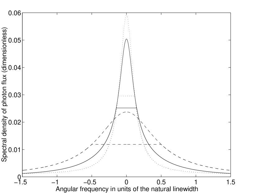
Figure 4: Plot of the Power Spectrum $P(\omega)$ of the fluorescence into the vacuum modes, for in-loop squeezing (solid) and free squeezing (dotted), with mode-matching $\eta=0.8$ and squeezing $S^{X}_{\rm in}(\bar{\omega})=0.05$. The linewidth for in-loop squeezing is slightly broader because the contribution from $\sigma_{y}$ is not broadened in this case. The natural-width spectrum from weak thermal driving (dashed) is scaled up for comparison

9.3 Comparison with Free Squeezing.

To compare the above results with those produced by free squeezing we again assume that the mode-matching of the squeezed modes into the atom is $\eta$, and that the squeezing is broad-band compared to the atom. Assuming also that the input light is in a minimum-uncertainty state for the $X$ and $Y$ quadratures [1], it can be characterized by a single real number $L$, with

$$S_{\rm in}^{X}(\omega)=L=1/S_{\rm in}^{Y}(\omega).$$ (231)

This parameter is related to those of Sec. 7.4 by $L=2N+2M+1$, where $M^{2}=N(N+1)$ and $M$ is assumed real. This yields the master equation

$$\dot{\rho}=(1-\eta){\cal D}[\sigma]\rho+\frac{\eta}{4L}{\cal D}[(L+1)\sigma-(L-1)\sigma^{\dagger}]\rho,$$ (232)

which leads again to (219)–(221), but with

$$\gamma_{x} = \mbox{$\frac{1}{2}$}\left[(1-\eta)+\eta L\right],$$ (233)

$$\gamma_{y} = \mbox{$\frac{1}{2}$}\left[(1-\eta)+\eta L^{-1}\right],$$ (234)

$$\gamma_{z} = \gamma_{x}+\gamma_{y}\;,\;\;C=1.$$ (235)

For $L<1$ the decay of $\sigma_{x}$ is again inhibited. The crucial observation to be made is that the dependence of $\gamma_{x}$ on the degree of $X$ quadrature squeezing of the input light is exactly the same as for in-loop squeezing, as is seen by comparing (231) and (233) with (226). The only difference between the two cases is that $C$ is unaffected by the free squeezing and that $\gamma_{y}$ is not increased by the in-loop squeezing. The latter is a direct consequence of the fact that an in-loop field is not bound by the usual two-time uncertainty relations. The free squeezing fluorescence spectrum is again given by (229). This is also plotted in Fig. 4 for $\eta=0.8$ and $L=0.05$. As this figure shows, the spectra are certainly not identical, but the sub-natural linewidth is much the same in both.

To conclude, line-narrowing of an atom is not a diagnostic of free squeezing. Rather, it requires only temporal anticorrelations of one quadrature of the input field (for times much shorter than the atomic lifetime) such as can be produced by a negative electro-optic feedback loop. The dependence of the line-narrowing on the input squeezing and the degree of mode-matching is the same for in-loop squeezing as for free squeezing. Because the quadrature operators of an in-loop field do not obey the usual two-time commutation relations, the reduction in noise in one quadrature does not imply an increase in noise in the other. Hence the line-narrowing of one quadrature of the atomic dipole by in-loop squeezing does not entail the line-broadening of the other quadrature. What significance this difference has in the physics of more complex atomic interactions with squeezed light [60] is a question requiring much investigation.

In-loop squeezing is generally easier to produce than free squeezing for a number of reasons. First, in-loop squeezing does not require expensive and delicate sources such as nonlinear crystals, but rather off-the-shelf electronic and electro-optical equipment. Second, the amount of squeezing is limited only by the efficiency of the photodetection. For homodyne detection, as required here, an efficiency of 95% is readily obtainable [64] and would enable in-loop squeezing of 95%. Third, in-loop squeezing can be produced at any frequency for which a coherent source is available, so experiments could be conducted on any atomic transition. The one difficulty with in-loop squeezing is that it requires a feedback loop response time much shorter than an atomic lifetime, but this would not be a problem for metastable transitions. Thus as well as giving us a better theoretical understanding of the effects on matter of light with fluctuations below the standard quantum limit, in-loop squeezing should be a practical alternative to free squeezing in the experimental investigation of these effects.

9.4 Other Uses of “Squashed light”

The analysis given above is probably the most interesting application for squashed light proposed so far. However, it is worth pointing out that another conceivable application was suggested in [26]. This was in the context of a QND measurement of an the squashed in-loop quadrature. For a perfect QND device, such a measurement does not disturb the feedback loop. Now because the in-loop fluctuations are squashed, the readout from the QND device will have less noise than it would have without feedback. This is useful if the measurement is being made with the aim not of determining the in-loop intensity, but of determining the coupling constant between the in-loop light and the QND meter. For a given detector bandwidth, the squashing of intensity fluctuations would thus enable this parameter to be estimated more accurately. The improvement in accuracy would be limited only by the efficiency of the photodetectors used in the feedback loop, as in (206).

Another potential application for squashed light was proposed recently in [31]. Here the idea is to reduce radiation pressure fluctuations on a mirror by squashing the amplitude fluctuations. The feedback involves standard photodetection and an amplitude modulator. The point of reducing the radiation pressure fluctuations is again to allow a more accurate estimation of other parameters, namely the spectrum of the thermal noise in the mirror. In this case it turns out that in the optimal regime the fluctuations can at most be reduced by a factor of one half.

10 Conclusion

What then, can we say in conclusion about squeezing and feedback? The first and foremost fact is that, in the absence of any nonlinear optical elements, feedback cannot produce free squeezing. A nonlinear optical element is any element whose effect cannot be modeled by a displacement, rotation, or damping of the amplitude of the light. By free squeezing I mean squeezing whose existence can be verified by detection in a conventional (demolition) detector which is not part of the feedback loop. This includes both continuum squeezing and intracavity squeezing (which can be measured by dumping the light out of the cavity).

If there are nonlinear optical elements present then there are many interesting things one can achieve with feedback involving squeezing. First, if those elements are used to generate a squeezed beam which is split, then feedback (or indeed feedforward) onto an intensity modulator can effectively transfer amplitude squeezing electronically from the beam which is detected to the free beam. This was discussed in Sec. 3.7. Second, nonlinear optical elements can create quantum correlations between two beams. Then, even if the beams separately are not squeezed, feedback (or, equally effectively, feedforward) of the light from one beam can make the other beam squeezed. If they are squeezed, then feedback or feedforward can enhance this squeezing. A number of scenarios were discussed in Sec. 5. Third, if the nonlinear element creates squeezing within a cavity then controlling the driving of the cavity by a photocurrent derived from a homodyne measurement of the output can enhance the squeezing, as discussed in Sec. 7. This could be seen as a generalization of the first case discussed above, where the cavity mirror is acting as a beam splitter and the intracavity light is being continually split.

A quite separate issue is the nature of the light within a feedback loop. At first sight it appears easy to make this squeezed, as negative feedback (without the aid of any optical nonlinearity) can produce an in-loop photocurrent with arbitrarily low noise, regardless of the efficiency of the detector. However, the fact that this is the current from an in-loop detector means that a sub-shot-noise spectrum does not have the usual significance. First, there is a perfectly good semiclassical explanation for this phenomenon in terms of coherent field states. Second, the usual two-time commutation relations for a free field do not hold for an in-loop field. This means that there is no “squeezing” of the uncertainty from the amplitude to the phase quadrature, rather just an apparent “squashing” of the amplitude uncertainty with no effect on the phase uncertainty. Lastly, from a practical point of view, the squeezed light cannot be removed from the loop using a linear optical device. A beam splitter inserted in the in-loop beam produces a free (out-of-loop) beam with noise level above rather than below the shot noise.

Despite the differences between in-loop squashing and free squeezing, it turns out that there are similarities. An in-loop quantum non-demolition amplitude detector will respond to amplitude squashing exactly as to amplitude squeezing. For a feedback loop constructed using a perfectly efficient (demolition) detection, a perfect in-loop non-demolition detector will have a read-out identical to that of the in-loop demolition detector, and, for arbitrarily large negative feedback, this will have an arbitrarily low noise level. For non-unit efficiency of the demolition detector in the feedback loop, the two detectors will not agree and the maximum degree of squashing observed by the non-demolition detector will be limited by the demolition detector efficiency.

The degree of squashing seen by a perfect QND detector turns out to be a legitimate measure of the degree of noise reduction in the light, and this squashing can have effects on nonlinear optical devices very similar to those produced by squeezing. In particular, shining broad-band quadrature squashed light on a resonant two-level atom will cause the decay of the in-phase quadrature of the atomic dipole to be suppressed. This manifest itself as a line-narrowing in the power spectrum of the atom’s fluorescence, an effect which was originally thought to be characteristic of squeezing. Moreover, the reduction in the linewidth of the in-phase quadrature depends on the degree of squashing (as measured by a QND device) in precisely the same way as it does on the degree of squeezing in the case of freely propagating light. This has important experimental implications as there are are a number of factors which make squashing easier to achieve than squeezing.

Very recently, there have been more intriguing developments in the theory of squashed light and its application to quantum spectroscopy [65]. First, I showed that it is possible to squash light simultaneously in both quadratures, and also to squeeze light in one quadrature and squash it the other. In the limit of perfect squeezing, and perfect squashing (which requires unit efficiency detectors) the in-loop fluctuations can be banished from both quadratures! An atom coupled only to this in-loop light would (to a first approximation) have its spontaneous decay completely suppressed. This surprising prediction is one more example of the continuing fruitful investigation of the relationship between feedback and squeezing.

Acknowledgment

I would like to thank Laura Thomsen for a careful reading of this manuscript. In work subsequent to the completion of this manuscript, we have generalized the work described above by considering the effect of twin-beam squashed light on a three-level atom [66]. We have also shown how feedback can be used to prepare near-minimum uncertainty spin-squeezed states [67].

References

- [1] D. F. Walls and G. J. Milburn, Quantum Optics (Springer, Berlin, 1994).
- [2] C. W. Gardiner, Quantum Noise (Springer, Berlin, 1991).
- [3] H. M. Wiseman and G. J. Milburn, Phys. Rev. A 49, 4110 (1994).
- [4] J. G. Walker and E. Jakeman, Proc. Soc. Photo-Opt. Instrum. Eng. 492, 274 (1985).
- [5] S. Machida and Y. Yamamoto, Opt. Commun. 55, 219 (1985).
- [6] H. A. Haus and Y. Yamamoto, Phys. Rev. A 34, 270 (1986).
- [7] Y. Yamamoto, N. Imoto and S. Machida, Phys. Rev. A 33, 3243 (1986).
- [8] J. M. Shapiro et al, J. Opt. Soc. Am. B 4, 1604 (1987).
- [9] H. J. Carmichael, L. Tian, W. Ren and P. Alsing, in Cavity QED, ed. Paul Berman, vol. 34 of Advances in AMO Physics (1994).
- [10] H. M. Wiseman and G. J. Milburn, Phys. Rev. Lett. 70, 548 (1993).
- [11] H. M. Wiseman and G. J. Milburn, Phys. Rev. A 49, 1350 (1994).
- [12] H. M. Wiseman, Phys. Rev. A 49, 2133 (1994).
- [13] H. J. Carmichael, An Open Systems Approach to Quantum Optics (Springer, Berlin, 1993).
- [14] C. W. Gardiner, A. S. Parkins and P. Zoller, Phys. Rev. A 46, 4363 (1992).
- [15] H. M. Wiseman and G. J. Milburn, Phys. Rev. A 47, 1652 (1993).
- [16] L. Plimak, Phys. Rev. A 50, 2120 (1994).
- [17] R. J. Glauber, Phys. Rev. 130, 2529 (1963).
- [18] R. J. Glauber, Phys. Rev. 131, 2766 (1963).
- [19] E. C. G. Sudarshan, Phys. Rev. Lett. 10, 277 (1963).
- [20] A. S. Troshin, Opt. Spektrosc. (USSR) 70, 389 (1991).
- [21] A. Heidmann and J. Mertz, J. Opt. Soc. Am. B 10, 1637 (1993).
- [22] C. Cohen-Tannoudji, J. Dupont Roc and G. Grynberg, Photons and Atoms: An Introduction to Quantum Electrodynamics (Wiley, New York, 1989).
- [23] C. W. Gardiner and M. J. Collett, Phys. Rev. A 31, 3761 (1985).
- [24] K. Mølmer, Phys. Rev. A 55, 3195 (1996).
- [25] H. P. Yuen and J. H. Shapiro, IEEE Trans. IT 26, 78 (1980).
- [26] M. S. Taubman et al. J. Opt. Soc. Am. B 12, 1792 (1995).
- [27] A. V. Masalov, A. A. Putilin and M. V. Vasilyev, J. Mod. Opt. 41, 1941 (1994).
- [28] J. J. Stefano, A. R. Subberud, and I. J. Williams, Theory and Problems of Feedback and Control Systems 2e (Mc Graw-Hill, New York, 1990).
- [29] Ya. A. Fananov, Opt. Spektrosc. (USSR) 70, 392 (1991).
- [30] S.-H. Youn et al. J. Opt. Soc. Am. B 11, 102 (1994).
- [31] B. C. Buchler et al., Opt. Lett. 24, 259 (1999).
- [32] D. B. Khoroshko and S. Ya. Kilin, JETP 79, 691 (1994).
- [33] M.S. Taubman et al., Proceedings of the 12th International Congress on Lasers in Research and Engineering (Springer, Berlin, 1996).
- [34] M. Hillery and M.O. Scully, Phys. Rev. D 25, 3137 (1982).
- [35] B. Yurke, J. Opt. Soc. Am. B2, 732 (1985).
- [36] P. Alsing, G. J. Milburn and D. F. Walls Phys. Rev. A 37, 2970 (1988).
- [37] E. Jakeman and J. G. Walker, Opt. Commun. 55, 219 (1985).
- [38] J. G. Walker and E. Jakeman, Optica-Acta. 32, 1303 (1985)
- [39] P. R. Tapster, J. G. Rarity and J. S. Satchell, Phys. Rev. A 37, 2963 (1988).
- [40] J. Mertz, A. Heidmann, C. Fabre, E. Giacobino and S. Reynaud, Phys. Rev. Lett. 64, 2897 (1990).
- [41] J. Mertz, A. Heidmann and C. Fabre, Phys. Rev. A 44, 3329 (1991).
- [42] M. J. Collett and R. B. Levien, Phys. Rev. A 43, 5068 (1991)
- [43] H. M. Wiseman, M. S. Taubman and H.-A. Bachor, Phys. Rev. A 51 3227 (1995).
- [44] R. Paschotta et al, Phys. Rev. Lett. 72, 3807 (1994)
- [45] G. Lindblad, Commun. Math. Phys. 48, 199 (1976).
- [46] J. von Neumann, Mathematical Foundations of Quantum Mechanics (Springer, Berlin, 1932); English translation (Princeton University Press, Princeton, 1955).
- [47] J. Dalibard, Y. Castin and K. Mølmer, Phys. Rev. Lett. 68, 580 (1992).
- [48] K. Mølmer, Y. Castin and J. Dalibard, J. Opt. Soc. Am. B 10, 524 (1993).
- [49] R. Dum, P. Zoller and H. Ritsch, Phys. Rev. A 45, 4879 (1992).
- [50] R. Dum, A. S. Parkins, P. Zoller and C. W. Gardiner, Phys. Rev. A 46, 4382 (1992).
- [51] L. Tian and H. J. Carmichael, Phys. Rev. A 46, R6801 (1992).
- [52] P. Marte, R. Dum, R. Taïeb and P. Zoller, Phys. Rev. A 47, 1378 (1993).
- [53] H. M. Wiseman and G. J. Milburn, Phys. Rev. A 47, 642 (1993).
- [54] C. W. Gardiner, Handbook of Stochastic Methods (Springer, Berlin, 1985).
- [55] V. Giovannetti, P. Tombesi and D. Vitali, quant-ph/9902077
- [56] P. Tombesi and D. Vitali, Phys. Rev. A 50, 4253 (1994).
- [57] P. Filipowicz, J. Javanainen and P. Meystre, Phys. Rev. A 34, 3077 (1986).
- [58] A. Liebman and G. J. Milburn, Phys. Rev. A 51, 736 (1995).
- [59] C. W. Gardiner, Phys. Rev. Lett. 56, 1917 (1986).
- [60] Z. Ficek and P. D. Drummond, Phys. Today 50, 34 (1997).
- [61] H. M. Wiseman, Phys. Rev. Lett. 81, 3840 (1998).
- [62] S.J. van Enk and H.J. Kimble, quant-ph/9908082.
- [63] D. W. Vernoy et al., Phys. Rev. A 57, R2293 (1998).
- [64] S. Schiller et al., Phys. Rev. Lett. 77, 2933 (1996).
- [65] H. M. Wiseman, J. Opt. B: Quant. Semiclass. Opt. 1, 459 (1999).
- [66] L.K. Thomsen and H.M. Wiseman, Phys. Rev. A 64, 043805 (2001).
- [67] L.K. Thomsen, S. Mancini, and H.M. Wiseman, Phys. Rev. A (Rapid Comm.) 65, 061801 (2002).