Atom correlations and spin squeezing near the Heisenberg limit: finite size effect and decoherence

Abstract

We analyze a model for spin squeezing based on the so-called counter-twisting Hamiltonian, including the effects of dissipation and finite system size. We discuss the conditions under which the Heisenberg limit, i.e. phase sensitivity $\propto 1/N$, can be achieved. A specific implementation of this model based on atom-atom interactions via quantized photon exchange is presented in detail. The resulting excitation corresponds to the creation of spin-flipped atomic pairs and can be used for fast generation of entangled atomic ensembles, spin squeezing and applications in quantum information processing. The conditions for achieving strong spin squeezing with this mechanism are also analyzed.

I Introduction

Interacting quantum systems that start in uncorrelated states generally evolve towards entangled states due to quantum correlations building up in time. These correlations and the form they take depend crucially on the interaction that gives rise to them. For example in parametric down conversion or in the optical parametric oscillator (OPO) pairs of photons can be created in distinct modes of the electromagnetic field. The fact that pairs of photons are generated leads to quantum correlations between the two modes. Since each mode is described by a harmonic oscillator, one can think of the state of the field as the quantum state of two fictitious particles in harmonic oscillator potentials. The quantum correlations correspond to e.g. the positions of the particles being strongly correlated, in the ideal case $\Delta(X_{1}-X_{2})^{2}\rightarrow 0$ and their momenta being anticorrelated $\Delta(P_{1}+P_{2})^{2}\rightarrow 0$. For the electromagnetic field modes, the position and momenta correspond to quadratures of the field modes and it is between these that correlations are produced [1, 2]. These correlations are essential to quantum communication e.g. quantum teleportation of information from one location to another [3]. Entanglement is also crucial for many schemes in quantum cryptography and for long-distance quantum communication through lossy channels [4].

Since the mechanism for producing correlations in electromagnetic field modes is at the fundamental level so simple (photons created in pairs) it is natural to wonder if such a simple mechanism may lead to entanglement of atoms interacting in a similar manner. In complete analogy to the OPA mechanism, a process that transfers pairs of atoms from their ground state to two well defined final states also gives rise to quantum correlations between atoms. When a collection of $N$ two level atoms is thought of as an ensemble of effective spin ${\frac{1}{2}}$ particles with total pseudo-angular momentum $J=N/2$, it turns out [5] that the quantum correlations produced by an interaction that transfers atoms in pairs from the lower state to the upper state shows up as reduced fluctuations in a component of the angular momentum e.g. $\Delta J_{x}^{2}\rightarrow 0$. We will discuss entanglement of atoms with one another in an atomic ensemble for which an effective interaction leads to the transfer of atoms in pairs to well defined final states and we will use the concept of spin squeezing to quantify the amount of quantum correlations produced in such a case. As for squeezed states of light, decoherence mechanisms and dissipation are acting in such a way as to destroy or limit the amount of squeezing achievable in practice. We also analyze the influence of such dissipation mechanisms and find relations between the spin squeezing interaction rate, the dissipation rate and the amount of squeezing achievable in the presence of damping mechanisms. The coherent control of the dynamical evolution of complex systems such as atomic ensembles may lead to the production of entangled non-classical states such as spin squeezed states [5] (analogous to squeezed states of light [2]) and correlated collective atomic modes (similar to twin photons generated by a non-degenerate OPO).

The main result of this paper is that for a collection of $N$ atoms with average single atom nonlinearity $\chi$ (two atom interaction energy) and with single atom loss rate $\Gamma$, the condition for achieving some spin squeezing is that $N\chi>\Gamma$. In order to achieve reduction of uncertainty in say $J_{x}$ compared to the uncertainty in the Bloch state $|J=N/2,J_{z}=N/2\rangle$ for which $(\Delta J_{x})^{2}=N/4$ by an amount $s$ (i.e. $(\Delta J_{x})^{2}=N/(4s)$) with $1\leq s\leq N$, one requires that $N\chi>s\Gamma$ and the interaction time needed scales as $t\sim(\log{s})/(N\chi)$ while the maximum number of atoms than can be lost without destroying the squeezing scales as $\Delta N\sim(N/s)\log{s}$. To achieve Heisenberg limited precision (i.e. maximum spin squeezing $s\sim N$), one needs a large single atom nonlinearity $\chi>\Gamma$. This means that the interaction time needed to achieve this strongly correlated state is $t\sim(\log{N})/(N\chi)$ and the maximum number of atoms that can be lost without compromising this optimal squeezing is $\Delta N\sim\log{N}$ i.e. a very small number of atoms lost may prevent reaching the Heisenberg limit. This analysis remains valid and agrees with a specific implementation based on an effective atom-atom interaction via quantized photon exchange in a cavity, for which the decoherence mechanism corresponds to spontaneous emission and leakage of photons from the cavity.

The possibility of coherently controlling interacting quantum systems has lead to many new developments in the field of quantum information science [6]. These are expected to have an impact in a broad area ranging from quantum computation and quantum communication [7] to precision measurements [8] and controlled modeling of complex quantum phenomena [9]. Entangled systems realized in the laboratory range in size from few qbits [10], to macroscopic ensemble of particles [11]. Controllable coherent interactions between atoms [12, 13] may also open the way for modelling of complex quantum phenomena such as quantum phase transitions [9] in which quantum correlations play a crucial role.

Entanglement of a single atomic ensemble, i.e. quantum correlations between atoms in the same ensemble, has been shown to be potentially very useful in the field of precision measurements [8]. Certain types of interactions between atoms lead to entanglement and spin squeezing, characterized by reduced variance in an observable and increased fluctuations in the canonically conjugate observable. This reduction of fluctuations directly translates into an improved accuracy for measurements sensitive to that observable. A typical figure of merit for spin squeezed states is the phase accuracy $\delta\phi$ on estimating accumulated dynamical phase in the Ramsey interferometric experiment. With all experimental uncertainties controlled below this noise level, the dominant source of noise in such experiments is the “quantum projection noise” [8] associated with e.g. the noise in measurements of the x-component of the spin of an ensemble of two-level atoms (effective spin ${\frac{1}{2}}$) all prepared in the lower level (the $|\downarrow\rangle$ state). This noise leads to a lower limit on phase accuracy $\delta\phi=1/\sqrt{N}$ called the standard quantum limit (SQL), where $N$ is the number of atoms in the ensemble. The Heisenberg uncertainty principle however allows for phase accuracies consistent with the basic principles of quantum mechanics that are as low as $\delta\phi=1/N$, called the Heisenberg limit.

We also discuss in more detail a technique [14] based on a resonantly enhanced nonlinear process involving Raman scattering into a “slow” optical mode [15], which creates a pair of spin-flipped atom and slowly propagating coupled excitation of light and matter (dark-state polariton). When the group velocity of the polariton is reduced to zero [16, 17], this results in pairs of spin flipped atoms. The dark-state polariton can be easily converted into corresponding states of photon wavepackets “on demand” [17], which makes the present approach most suitable for implementing protocols in quantum information processing that require a combination of deterministic sources of entangled states and long-lived quantum memory [4, 18].

This paper is divided into V sections. In Section II, we discuss Ramsey spectroscopy and the use of spin-squeezed states in precision measurements. In particular we analyze the situation where $N$ two level atoms with levels $|g\rangle$ and $|e\rangle$ are prepared in a correlated state and subsequently probed by separated fields of frequency $\omega$ in the Ramsey interferometric configuration, which we review in Appendix A. We also discuss spin-squeezed states and develop pictorial representation of those states which we compare to squeezed states of light and in appendix B we introduce the Wigner representation for a particular class of spin squezed states.

In Section III, we analyze a model for spin squeezing based on the analogy with the optical parametric oscillator. We also seek to understand the influence of loss processes on the coherent spin-squeezing interaction and the way in which it limits the correlations achievable for a given interaction rate. The model consists of two bosonic modes (a “spin up” state and a “spin down” state) with loss rates and a coherent interaction that transfers pairs of atoms from one mode to the other. For our simple model, analytical results can be obtained in the perturbative regime of small number of excitations (most atoms in the lower state) and low loss rate. We estimate the conditions for which Heisenberg-limited spin squeezed states can be produced.

In Section IV, we present a scheme for inducing effective coherent interactions between atoms in an atomic ensemble. These coherent interactions lead to massive entanglement of the ensemble and to characterize the degree of entanglement thus obtained, we calculate the squeezing or reduction in fluctuations of one particular observable. The coherent interaction is based on Raman scattering into a cavity mode for which the atomic medium is made transparent by Electromagnetically Induced Transparency (EIT). The slowly propagating mode is then best described by a polariton: a collective excitation that is partly photonic and partly “spin” excitation of the atomic ensemble (the up and down states of the spin being two metastable states). The overall process leads to the creation of pairs of excitations, one being a “spin flip” created by Raman scattering, the other being a polariton which can be “steered” into a photon or spin flip excitation “on demand”. We find that substantial spin squeezing can be obtained for atomic ensembles in low finesse cavities, without the strong coupling requirement of cavity QED. In the limit of unity finesse this corresponds to free-space configuration and substantial correlations can still be produced in this case. In the opposite limit of high finesse, very strong correlations are obtained and in particular we estimate the regime for which Heisenberg limited spin-squeezed states are produced.

II Ramsey spectroscopy with correlated atoms

In appendix A, Ramsey spectroscopy is reviewed and in particular we show how the phase accuracy in phase estimation based on the Ramsey fringe signal is, at the maximum sensitivity point, given by

$$\delta\phi=\frac{\Delta J_{x}}{|\langle\hat{J}_{z}\rangle|}$$ (1)

where $\Delta J_{x}$ is the variance in the x-component of the pseudo angular momentum (of length $J=N/2$) representing the state of $N$ two-level atoms and $\langle\hat{J}_{z}\rangle$ is the expectation value of the z-component of the pseudo angular momentum (both the variance and the expectation value are calculated in the initial state).

For an uncorrelated state of atoms e.g. with all atoms in their lower state so that the state of the ensemble is described by $|J_{z}=-N/2\rangle$, it is found that $\Delta J_{x}=\sqrt{J/2}$ and $\langle\hat{J}_{z}\rangle=-J$ so that $\delta\phi=\sqrt{1/N}$. In order to improve the phase accuracy, one must use a state for which the variance in $\hat{J}_{x}$ is reduced while $\langle\hat{J}_{z}\rangle$ is little changed. Consider therefore a state such as an eigenstate of $\hat{J}_{x}$, for example $|J_{x}=0\rangle$. Calculating the expectation values and variances we find $\langle\hat{J}_{x}\rangle=\langle\hat{J}_{y}\rangle=\langle\hat{J}_{z}\rangle=0$, $\Delta J_{x}=0$ and $\Delta J_{y}=\Delta J_{z}=\sqrt{J(J+1)/2}$. However the Ramsey signal has amplitude proportional to $\langle J_{z}\rangle$ and therefore vanishes for all phase angles $\phi$, which means that even though the noise or fluctuation properties of the signal may be improved, its average is zero. Note that this is because we have chosen $\hat{J}_{z}(\phi)$ as our observable, other observables such as $\hat{J}_{z}^{2}(\phi)$ for example may lead to non-zero average signal together with reduced variance [19, 20]. However, it turns out their signal to noise ratio is very much reduced compared to that of the Ramsey scheme [20]. It is thus necessary to consider states that lead to a reduced variance $\Delta J_{x}$ while maintaining a large signal amplitude, i.e. a large $\langle\hat{J}_{z}\rangle$. We therefore consider states such as

$$|\psi(a)\rangle=\frac{1}{\sqrt{1+a^{2}}}(i|J_{x}=0\rangle+a\frac{|J_{x}=+1\rangle-|J_{x}=-1\rangle}{\sqrt{2}})$$ (2)

where $a$ is a real number parametrizing the state $|\psi(a)\rangle$. It is straightforward to calculate the expectation values

$$\langle\hat{J}_{x}\rangle = 0$$ (3)

$$\langle\hat{J}_{y}\rangle = 0$$ (4)

$$\langle\hat{J}_{z}\rangle = \frac{2a}{1+a^{2}}\sqrt{\frac{J(J+1)}{2}}$$ (5)

and the variances

$$\Delta J_{x} = \frac{a}{\sqrt{1+a^{2}}}$$ (6)

$$\Delta J_{y} = \frac{1}{\sqrt{1+a^{2}}}\sqrt{\frac{J(J+1)}{2}}$$ (7)

$$\Delta J_{z} = \sqrt{\frac{J(J+1)}{2}}\left[1-\frac{4a^{2}}{(1+a^{2})^{2}}\right]^{1/2}.$$ (8)

FIG. 1.: Number of atoms detected in the upper state ($N_{e}$) relative to total number of atoms (the total number is $N=N_{e}+N_{g}$ and thus $N_{e}/(N_{e}+N_{g})=(N/2+\langle J_{z}(\phi)\rangle)/N$) vs. accumulated phase $\phi=(\omega-\omega_{0})T$ for a) uncorrelated atoms and b) correlated atoms in a spin-squeezed state $|\psi(a)\rangle$, for $N=100$ and $a=-1.1$ (note that error bars have been magnified by a factor of $10$ for clarity). Note how squeezing of the variance improves the phase accuracy.

The signal amplitude which depends on $\langle\hat{J}_{z}\rangle$ can thus be rather large ($O[N]$) while the noise amplitude characterized by $\Delta J_{x}$ is minimized ($O[1]$). The Ramsey signal and phase accuracy for such a state is shown in Fig. 1b, compared to the case of uncorrelated atoms (Fig. 1a).

These states are minimum uncertainty states i.e. $(\Delta J_{x})(\Delta J_{y})={\frac{1}{2}}|\langle\hat{J}_{z}\rangle|$ for all values of the parameter $a$. Also, their phase accuracy is given by

$$\delta\phi(\pm\pi/2)=\sqrt{\frac{1+a^{2}}{2}}\frac{1}{\sqrt{J(J+1)}}$$ (9)

which is of order $1/N$. The best phase accuracy is obtained for $a\rightarrow 0$ in which case the optimal phase accuracy is $\delta\phi(\pm\pi/2)=\sqrt{2}/N$. Note that in this case the signal amplitude ($\propto\langle\hat{J}_{z}\rangle$) becomes vanishingly small ($\langle\hat{J}_{z}(\phi)\rangle\rightarrow 0$ for all $\phi$) and also the range of values of $\phi$ for which improved phase accuracy is achieved becomes vanishingly small around $\phi=\pm\pi/2$. For these reasons, the optimally spin squeezed state $|\psi(a=0)\rangle$ may prove impractical. Note however that for finite $a$ i.e. for $|a|=1$, the signal amplitude is large ($\sim N/\sqrt{8}$) and the phase accuracy is independent of $\phi$

$$\delta\phi(\phi)=\frac{1}{\sqrt{J(J+1)}}\simeq\frac{2}{N}$$ (10)

i.e. twice the Heisenberg limit.

FIG. 2.: Number of atoms detected in the upper state vs. accumulated phase $\phi=(\omega-\omega_{0})T$ for correlated atoms in various spin-squeezed states $|\psi(a)\rangle$, for $N=100$ and $a=-0.9$, $a=-1$ and $a=-1.1$. Also shown is the phase accuracy $\delta\phi(\phi)$ vs. accumulated phase (the dashed line represents the standard quantum limit $\delta\phi=1/\sqrt{N}$). Note how $\delta\phi(\phi)$ gets to a minimum value of order $2/N=0.02$.

In Fig. 2 we show the signal and variance for various spin squeezed states along with the phase accuracy $\delta\phi(\phi)$.

We can gain a better understanding of the squeezing in the states (2) $|\psi(a)\rangle$ by looking at various representations of them. The simplest representation is to project the state onto eigenstates of the three components of the angular momentum

$$P_{i}(m)=|\langle J_{i}=m|\psi(a)\rangle|^{2}$$ (11)

where $|J_{i}=m\rangle$ is the eigenstate of the i-component of angular momentum with eigenvalue $m$.

From Fig. 3 it is clear that the expectation value of $\hat{J}_{x}$ and $\hat{J}_{y}$ are zero in such a state, whereas (for $a=-1$) the expectation value of $\hat{J}_{z}$ is large and negative, the variances are clearly given by (8). It is interesting to note the similarity of these angular momentum squeezed states and those of a harmonic oscillator (i.e. squeezed states of light). In both cases, the probability distributions vanish for odd number of quanta (note that for simplicity we consider only $N$ even here).

FIG. 3.: Projection of the state $|\psi(a)\rangle$ onto eigenstates of the angular momentum operators $\hat{J}_{x}$, $\hat{J}_{y}$ and $\hat{J}_{z}$ for $J=N/2=20$ and $a=-1$. The $P_{x}(m)$ distribution is sharply peaked since the state $|\psi(a)\rangle$ is a superposition of the $m_{x}=-1,0,+1$ components only; the $P_{y}(m)$ distribution is broad and symmetric; the $P_{z}(m)$ distribution vanishes for $m$ odd and the even components decrease roughly exponentially with $m$.

For even number of quanta, the behaviour is nearly exponential $P_{z}(m)\propto e^{-c(m+j)}$ for some constant $c$. A mechanism for generating such states starting from the uncorrelated state $|J_{z}=-J\rangle$ must therefore be one in which atoms are excited in pairs, i.e. two atoms in the ground state are transferred to the excited state $|g\rangle|g\rangle\rightarrow|e\rangle|e\rangle$. Consider the similarities with squeezed states of light: in particular the photon number distribution vanishes for odd photon number in the case of squeezed vacuum due to the form of the squeezing Hamiltonian $\hat{H}=-i\chi[\hat{a}^{\dagger 2}-\hat{a}^{2}]$, which creates and destroys photons in pairs. Since we find a similar cancellation of the probability of there being odd number of excitations for the states $|\psi(a)\rangle$, the interaction giving rise to such states starting from all atoms in their lower states must likewise create and destroy excitations in pairs and thus be of the form $\hat{H}=-i\hbar\chi[\hat{L}_{+}^{2}-\hat{L}_{-}^{2}]$. This process can also be viewed as a coherent collision mechanism. Moreover, for the whole atomic ensemble to become entangled (not just particular atom pairs), this process must occur completely symmetrically for all atoms. It should not be two particular atoms that get transferred to the excited state, rather it should be two collective excitations that get created

$$|g_{1}\cdots g_{N}\rangle \rightarrow \sqrt{\frac{2}{N(N-1)}}\sum_{i>j}\left[|g\cdots e_{i}\cdots e_{j}\cdots g\rangle\right]$$ (12)

which is the state obtained by letting $\hat{J}_{+}^{2}$ operate on $|J_{z}=-J\rangle$. The simplest Hamiltonian giving rise to this type of interaction is analyzed in section III to quantify the squeezing generated by this mechanism. This form of interaction was considered by Kitegawa and Ueda [5] in their classic study of spin squeezing and was dubbed the “two axis countertwisting” interaction.

III Two axis counter twisting model

We now turn to the analysis of the two axis countertwisting Hamiltonian [5]

$$\hat{H} = -i\frac{\hbar\chi}{2}\left(\hat{L}_{+}^{2}-\hat{L}_{-}^{2}\right)$$ (13)

$$= \hbar\chi\left(\hat{L}_{x}\hat{L}_{y}+\hat{L}_{y}\hat{L}_{x}\right).$$ (14)

As argued in last section it is this type of Hamiltonian that most closely parallels squeezed state generation for light.

We now present a general theory that allows to quantify atom correlations and takes into account decoherence and finite system size. Specifically, we consider two bosonic modes (such as for a two component Bose-Einstein condensate or for an atomic ensemble with two relevant atomic levels) with annihilation operators $\hat{a}_{1}$ and $\hat{a}_{2}$. The system is also subject to damping i.e. loss of atoms at rates which may depend on the internal state. The equations of motion for the two modes are then (with $\hat{L}_{+}=\hat{a}_{2}^{\dagger}\hat{a}_{1}$ and $\hat{L}_{-}=\hat{a}_{1}^{\dagger}\hat{a}_{2}$)

$$\dot{\hat{a}}_{1}=-\gamma_{1}\hat{a}_{1}+\chi\hat{a}_{1}^{\dagger}\hat{a}_{2}^{2}+\hat{F}_{1}(t)$$ (15)

$$\dot{\hat{a}}_{2}=-\gamma_{2}\hat{a}_{2}-\chi\hat{a}_{2}^{\dagger}\hat{a}_{1}^{2}+\hat{F}_{2}(t)$$ (16)

where $\hat{F}_{j}(t)$ are delta-correlated Langevin noise forces with appropriate diffusion coefficients $D_{ij}=\langle\hat{F}_{i}(t)\hat{F}_{j}(t)\rangle$.

In order to discuss spin squeezing, it is easier to rewrite the equations of motion in terms of the Stokes parameters

$$\hat{L}_{0} = \hat{N}=\hat{a}_{1}^{\dagger}\hat{a}_{1}+\hat{a}_{2}^{\dagger}\hat{a}_{2}$$ (17)

$$\hat{L}_{x} = (\hat{a}_{2}^{\dagger}\hat{a}_{1}+\hat{a}_{1}^{\dagger}\hat{a}_{2})/2$$ (18)

$$\hat{L}_{y} = (\hat{a}_{2}^{\dagger}\hat{a}_{1}-\hat{a}_{1}^{\dagger}\hat{a}_{2})/2i$$ (19)

$$\hat{L}_{z} = (\hat{a}_{2}^{\dagger}\hat{a}_{2}-\hat{a}_{1}^{\dagger}\hat{a}_{1})/2$$ (20)

for which the equations are

$$\dot{\hat{L}}_{0} = -2\Gamma\hat{L}_{0}+4\gamma\hat{L}_{z}+\hat{F}_{0}(t)$$ (21)

$$\dot{\hat{L}}_{x} = -2\Gamma\hat{L}_{x}+\chi(\hat{L}_{x}\hat{L}_{z}+\hat{L}_{z}\hat{L}_{x})+\hat{F}_{x}(t)$$ (22)

$$\dot{\hat{L}}_{y} = -2\Gamma\hat{L}_{y}-\chi(\hat{L}_{y}\hat{L}_{z}+\hat{L}_{z}\hat{L}_{y})+\hat{F}_{y}(t)$$ (23)

$$\dot{\hat{L}}_{z} = -2\Gamma\hat{L}_{z}+\gamma\hat{L}_{0}-2\chi(\hat{L}_{x}^{2}-\hat{L}_{y}^{2})+\hat{F}_{z}(t)$$ (24)

where $\Gamma=(\gamma_{1}+\gamma_{2})/2$, $\gamma=(\gamma_{1}-\gamma_{2})/2$ and $\hat{F}_{j}(t)$ are new delta-correlated noise forces associated with the damping.

Since (24) are non-linear operator equations, in the equations of motion for the first order moments $\langle\hat{L}_{i}\rangle$ there are terms that depend on those first order moments but also terms depending on the second order moments $\langle\hat{L}_{i}\hat{L}_{j}\rangle$. Similarly the equations of motion for the second order moments depend on themselves and also on the third order moments, and so on, leading to the BBGKY hierarchy of equations of motion for the expectation values of operator products. In order to solve this set of equations, the hierarchy must be truncated at some order [21]. Keeping the first and second order moments, we truncate the BBGKY hierarchy by the approximation

$$\langle\hat{L}_{i}\hat{L}_{j}\hat{L}_{k}\rangle \approx \langle\hat{L}_{i}\hat{L}_{j}\rangle\langle\hat{L}_{k}\rangle+\langle\hat{L}_{j}\hat{L}_{k}\rangle\langle\hat{L}_{i}\rangle+\langle\hat{L}_{k}\hat{L}_{i}\rangle\langle\hat{L}_{j}\rangle$$ (25)

$$- 2\langle\hat{L}_{i}\rangle\langle\hat{L}_{j}\rangle\langle\hat{L}_{k}\rangle.$$ (26)

The equations of motion for the expectation values $l_{i}\equiv\langle\hat{L}_{i}\rangle$ and the second order moments $\Delta_{ij}\equiv\langle\hat{L}_{i}\hat{L}_{j}+\hat{L}_{j}\hat{L}_{i}\rangle-2\langle\hat{L}_{i}\rangle\langle\hat{L}_{j}\rangle$ are then obtained from (24). We are interested in the case when all atoms start in mode $1$, i.e. $l_{0}(0)=N,l_{x}(0)=l_{y}(0)=0,l_{z}(0)=-N/2$ and $\Delta_{xx}(0)=\Delta_{yy}(0)=N/2$ (all other second moments vanish) and for simplicity we take $\gamma_{1}=\gamma_{2}=\Gamma$, $\gamma=0$. Writing only the relevant equations and omitting vanishing terms (such as those proportional to $\Delta_{xz}$ and $\Delta_{yz}$ which are zero for all times), we have (after some algebra)

$$\dot{l}_{0} = -2\Gamma l_{0}$$ (27)

$$\dot{l}_{z} = -2\Gamma l_{z}-\chi(\Delta_{xx}-\Delta_{yy})$$ (28)

$$\dot{\Delta}_{xx} = -4\Gamma\Delta_{xx}+\Gamma l_{0}+4\chi l_{z}\Delta_{xx}$$ (29)

$$\dot{\Delta}_{yy} = -4\Gamma\Delta_{yy}+\Gamma l_{0}-4\chi l_{z}\Delta_{yy}$$ (30)

and $l_{x}(t)=l_{y}(t)=0$. These equations are non-linear and cannot be solved analytically nor perturbatively in $\Gamma/\chi$. For short enough times, the number of excitations into mode $2$ is small and $l_{z}\simeq-N/2$, so that plugging this in (30) we have

$$\Delta_{xx}(t) \simeq {\frac{N}{2}}e^{-2N\chi t}+O[\Gamma/\chi]$$ (31)

$$\Delta_{yy}(t) \simeq {\frac{N}{2}}e^{2N\chi t}+O[\Gamma/\chi]$$ (32)

i.e. the variance of the x-component of the pseudo-angular momentum is squeezed while that of the y-component is anti-squeezed. Plugging these back in the equation of motion of $l_{z}$, we obtain $l_{z}(t)\simeq-N/2+(\cosh{2N\chi t}-1)/2+O[\Gamma/\chi]$. This equation predicts growth of $l_{z}$ without bound, however we know that because $l_{z}$ is the z-component of an angular momentum vector, we must have $|l_{z}|\leq N/2$. The phase space of this angular momentum vector is the Bloch sphere and in essence we have neglected the small curvature of the Bloch sphere (of radius $R=N/2$) and have approximated the phase space by the flat planar phase space of a harmonic oscillator. We call this approximation the bosonic approximation, since it predicts infinite squeezing in the long time limit and in the absence of dissipation, similar to the case of squeezed light. Formally this is equivalent to assuming

$$[\hat{a}_{2}^{\dagger}\hat{a}_{1},\hat{a}_{1}^{\dagger}\hat{a}_{2}] = \hat{a}_{2}^{\dagger}\hat{a}_{2}-\hat{a}_{1}^{\dagger}\hat{a}_{1}$$ (33)

$$\simeq -N$$ (34)

i.e. the operator $\hat{S}_{+}=\hat{a}_{2}^{\dagger}\hat{a}_{1}/\sqrt{N}$ obeys bosonic commutation relations. Under this approximation the Hamiltonian (14) becomes $\hat{H}=-i(\hbar\chi N/2)(\hat{S}_{+}^{2}-\hat{S}_{-}^{2})$ which is identical to the Hamiltonian describing squeezing of light [2].

In order to take into account the curvature of phase space and the non-bosonic nature of the angular momentum operators, we use the following transformation

$$\hat{N} = N\hat{h}_{0}$$ (35)

$$\hat{L}_{x} = \sqrt{N}\hat{h}_{x}$$ (36)

$$\hat{L}_{y} = \sqrt{N}\hat{h}_{y}$$ (37)

$$\hat{L}_{z} = \hat{h}_{z}-\frac{N}{2}\hat{h}_{0}$$ (38)

in terms of which the commutation relations become

$$\left[\hat{h}_{x,y,z},\hat{h}_{0}\right] = 0$$ (39)

$$\left[\hat{h}_{z},\hat{h}_{\pm}\right] = \pm\hat{h}_{\pm}$$ (40)

$$\left[\hat{h}_{+},\hat{h}_{-}\right] = 2\frac{\hat{h}_{z}}{N}-\hat{h}_{0}$$ (41)

where $\hat{h}_{\pm}=\hat{h}_{x}\pm i\hat{h}_{y}$. In the limit $N\rightarrow\infty$ these commutation relations become those of bosonic operators i.e. $\lim_{N\rightarrow\infty}[\hat{h}_{0},\hat{h}_{z},\hat{h}_{+},\hat{h}_{-}]=[\hat{1},\hat{a}^{\dagger}\hat{a},\hat{a}^{\dagger},\hat{a}]$, a process formally known as a group contraction [22]. The linear transformation of operators (38) does not introduce any extra approximation.

The Hamiltonian (14) can be re-expressed as

$$\hat{H} = \hbar\chi N\left(\hat{h}_{x}\hat{h}_{y}+\hat{h}_{y}\hat{h}_{x}\right)$$ (42)

$$= -i\frac{\hbar\xi}{2}\left(\hat{h}_{+}^{2}-\hat{h}_{-}^{2}\right)$$ (43)

where we have defined $\xi=\chi N$. We can now obtain equations of motion for the expectation values $h_{j}=\langle\hat{h}_{j}\rangle$ and the second order moments $\delta_{ij}=\langle\hat{h}_{i}\hat{h}_{j}\rangle-2\langle\hat{h}_{i}\rangle\langle\hat{h}_{j}\rangle$ from (30). Letting $\tau=N\chi t=\xi t$ be a rescaled time, $\kappa=\Gamma/(N\chi)=\Gamma/\xi$ be the rescaled dissipation rate and writing $\epsilon=1/N$ and $\dot{x}={\rm d}x/{\rm d\tau}$, we have

$$\dot{h}_{0} = -2\kappa h_{0}$$ (44)

$$\dot{h}_{z} = -2\kappa h_{z}-(\delta_{xx}-\delta_{yy})$$ (45)

$$\dot{\delta}_{xx} = -4\kappa\delta_{xx}+\kappa h_{0}-2h_{0}\delta_{xx}+4\epsilon h_{z}\delta_{xx}$$ (46)

$$\dot{\delta}_{yy} = -4\kappa\delta_{yy}+\kappa h_{0}+2h_{0}\delta_{yy}-4\epsilon h_{z}\delta_{yy}.$$ (47)

Note that these equations are formally equivalent to (30), no approximation has been made from (30) to (47). Letting $\epsilon\rightarrow 0$ reproduces the results of the bosonic approximation obtained above in the limit of $l_{z}\simeq-N/2$. Terms of order $\epsilon$ and higher represent corrections to the bosonic approximation and, as shown below, they give rise to a limit to the amount of squeezing achievable.

Solving (47) to first order in $\epsilon$ and $\kappa$ we obtain, writing only the relevant terms,

$$\delta_{xx}(\tau) = \frac{1}{2}\left[e^{-2\tau}+(\kappa+\epsilon/2)+\cdots\right]$$ (48)

which shows that the variance $\Delta J_{x}=\sqrt{(N/2)\delta_{xx}}$ is squeezed. Second order terms in $\kappa$ and $\epsilon$ come multiplied by an exponentially growing term $e^{2\tau}$ so that as a function of time, the variance reaches a minimum value $\delta_{xx}\sim{\rm max}[\kappa,\epsilon]$ at a time $e^{-\tau_{*}}\sim{\rm max}[\kappa,\epsilon]$, after which it grows exponentially and the squeezing is lost. Note that this behaviour ($\delta_{xx}(t)$ reaches a minimum value and then increases again) also occurs when $\kappa\rightarrow 0$, indicating that it is a generic feature of the finite system size. This model predicts that a variance $\delta_{xx}\sim\epsilon=1/N\rightarrow\Delta J_{x}^{2}\sim 1$ is achievable as long as losses are small enough, i.e. $\kappa\sim\epsilon$, which in terms of $\chi$ and $\Gamma$ means

$$\chi\sim\Gamma\;\;\;{\rm or}\;\;\xi\sim N\Gamma$$ (49)

where $\chi$ corresponds to the single-atom nonlinear interaction rate and $\Gamma$ represents the single-atom loss rate.

In order to achieve any squeezing ($\delta_{xx}\leq 1/2$) it is necessary to have $\kappa<1$ i.e. $N\chi>\Gamma$. In the regime $N\chi\gg\Gamma$ very strong correlations can be obtained. Note that the single-atom nonlinearity can still be relatively weak compared to the single particle loss rate ($\chi\ll\Gamma$). For example when the dissipation rate is such that $\kappa\sim\sqrt{\epsilon}$ i.e. $\sqrt{N}\chi\sim\Gamma$, the amount of squeezing obtained (48) is $\delta_{xx}\sim 1/\sqrt{N}$. It takes a time $e^{-2\tau}\sim\sqrt{\epsilon}$ to reach this state and the number of particles lost during that time is $\Delta N\sim N\times 2\kappa\tau\sim\sqrt{N}\log{N}$. This number can therefore also be thought of as the maximum number of particles that can be lost from the ensemble without destroying squeezing beyond $\delta_{xx}\sim 1/\sqrt{N}$.

In order to reach the Heisenberg limit it is required that the single atom nonlinearity $\chi$ be larger than the decay rate $\Gamma$. Note that in this case, the number of atoms lost by the time optimal squeezing is achieved is $\Delta N\sim\log{N}$ which indicates that a very small number of atoms is lost. This number also corresponds to the maximum number of particles that can be lost from the ensemble and not destroy squeezing at the Heisenberg limit level. Clearly the more squeezed the state of the atoms is, the more sensitive it becomes to atom loss and in general to any form of dissipation.

IV Coherent atom interactions via slow light

We now describe a technique to induce effective coherent interactions between atoms in metastable states [14]. The technique is based on a resonantly enhanced nonlinear process involving Raman scattering into a “slow” optical mode [15], which creates a pair of spin-flipped atom and slowly propagating coupled excitation of light and matter (dark-state polariton). When the group velocity of the polariton is reduced to zero [16, 17], this results in pairs of spin flipped atoms. The fact that pairs of atomic excitations are created in this process can also be viewed as a coherent interaction between atoms, i.e. a controlled “collision” leading to entanglement of the state of each atom with that of every other atom in the ensemble.

A number of proposals have been made for generating entangled states of atomic ensembles and resulting in so-called spin squeezed states. Some are based on interatomic interactions at ultra-cold temperatures [23], whereas others involve mapping the states of non-classical light fields into atoms [24], QND measurements of spins [25] with light or dipole blockade for Rydberg atoms [26]. In contrast to some of these mechanisms the present approach does not require coherence of the atomic motion or sources of non-classical light and is completely deterministic thereby significantly simplifying possible experimental realizations. We further show that the present technique can be made robust with respect to realistic decoherence processes such as spontaneous emission and leakage of slow photons from the medium.

We consider a system of $N$ atoms (Fig. 4a) interacting with two classical driving fields $\Omega_{1,2}$ and one quantized mode $\hat{a}$ of a running wave cavity that is initially in a vacuum state. Note that we consider a cavity configuration for ease of theorerical treatment, the results of this analysis however remain valid in the limit of unity finesse, i.e. in free space configuration. Relevant atomic sublevels include two manifolds of metastable states (e.g hyperfine sublevels of electronic ground state) and excited states that may be accessed by optical transitions. The atoms are initially prepared in their ground states $|g\rangle$. One of the classical fields, of Rabi frequency $\Omega_{1}$, is detuned from the atomic resonance by an amount roughly equal to the frequency splitting between ground state manifolds. The other field of Rabi frequency $\Omega_{2}$ is resonant with an atomic transition $|b_{2}\rangle\rightarrow|a_{2}\rangle$. The quantized field can be involved in two Raman transitions corresponding to Stokes and anti-Stokes processes. Whereas the former corresponds to the usual Stokes scattering in the forward direction, the latter establishes an Electromagnetically Induced Transparency (EIT) and its group velocity is therefore substantially reduced.

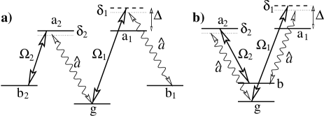
FIG. 4.: Energy levels scheme for the effective coherent interaction leading to creation of pairs of atoms a) in different final states (“non-degenerate” scheme) and b) in identical final states(“degenerate” version).

The pair excitation can be viewed as resulting from quantized photon exchange between atoms (Fig. 5) in a two-step process. The first flipped spin is created due to Stokes Raman scattering, which also results in photon emission in a corresponding Stokes mode. In the presence of EIT, this photon is directly converted into a dark-state polariton which becomes purely atomic when the group velocity is reduced to zero. This implies that atomic spins are always flipped in pairs. In Fig. 4a the two final states involved in Raman transitions are different and atomic pairs in different states are created. In Fig. 4b the final states of the two Raman processes are identical, in which case atomic pairs in the same state result. The analysis of this “degenerate” version of the scheme is similar to the “non-degenerate” case and we will consider only the latter case here.

FIG. 5.: Diagram illustrating coherent atom-atom interaction mediated by dark-state polariton, leading to the creation of a pair of spin-flipped atoms.

For conceptual simplicity we assume that the quantized field corresponds to a single mode of a running-wave cavity with a creation operator $\hat{a}^{\dagger}$ and atom-field coupling constants $g_{1}$ and $g_{2}$. The interaction Hamiltonian for the system of N atoms and light can be split into two parts $H=H_{Ram}+H_{res}$ corresponding to the Stokes Raman process and the anti-Stokes process respectively:

$$H_{Ram} = -\hbar\Delta\Sigma_{a1a1}-\hbar\delta_{1}\Sigma_{b_{1}b_{1}}$$ (50)

$$+ [\hbar\Omega_{1}\Sigma_{a_{1}g}+\hbar g_{1}a\Sigma_{a_{1}b_{1}}+{\rm h.c.}],$$ (51)

$$H_{res} = \hbar\delta_{2}\Sigma_{b_{2}b_{2}}+\hbar\delta_{2}\Sigma_{a_{2}a_{2}}$$ (52)

$$+ [\hbar g_{2}a\Sigma_{a_{2}g}+\hbar\Omega_{2}\Sigma_{a_{2}b_{2}}+{\rm h.c.}],$$ (53)

where $\Sigma_{\mu\nu}=\sum_{i}|\mu\rangle_{ii}\langle\nu|$ are collective atomic operators corresponding to transitions between atomic states $|\mu\rangle,|\nu\rangle$, $\Delta$ is the detuning of the classical field $\Omega_{1}$ from the single-photon transition $|g\rangle\rightarrow|a_{1}\rangle$, $\delta_{1}$ and $\delta_{2}$ are the two-photon detunings from the $|g\rangle\rightarrow|b_{1}\rangle$ and $|g\rangle\rightarrow|b_{2}\rangle$ transitions respectively as shown in Fig. 4.

In the limit of large detuning $\Delta$ and ignoring two-photon detunings for the moment, the Hamiltonian $H_{Ram}$ describes off-resonant Raman scattering. We take into account realistic decoherence mechanisms such as spontaneous emission from the excited states in all directions and decay of the cavity mode with a rate $\kappa$. The evolution of atomic operators is then described by Heisenberg-Langevin equations:

$${\dot{\Sigma}}_{\mu\nu}=-\gamma_{\mu\nu}\Sigma_{\mu\nu}+{i\over\hbar}[H,\Sigma_{\mu\nu}]+F_{\mu\nu},$$ (54)

where $\gamma_{\mu\nu}$ is a decay rate of coherence $\mu\rightarrow\nu$ and $F_{\mu\nu}$ are associated noise forces. The latter have zero average and are $\delta$-correlated with associated diffusion coefficients that can be found using the Einstein relations.

After a canonical transformation corresponding to adiabatic elimination of the excited state (see Appendix C for details), $H_{Ram}$ becomes equivalent to the effective Hamiltonian

$${\tilde{H}}_{Ram}=\hbar\chi\hat{a}^{\dagger}\hat{S}_{1}^{\dagger}+{\rm h.c.}$$ (55)

where $\hat{S}_{1}=\Sigma_{gb_{1}}/\sqrt{N}$ and $\chi=g_{1}\sqrt{N}\Omega_{1}^{*}/\Delta$. This effective hamiltonian thus describes the process in which a Stokes photon is emitted necessarily accompanied by a spin flip. The quantum state of the Stokes mode is thus perfectly correlated with the state of the atomic spin flip mode.

The resonant part of the Hamiltonian $H_{res}$ is best analyzed in terms of dark and bright-state polaritons [27]

$$P_{D} = {\Omega_{2}a-g_{2}\sqrt{N}S_{2}\over\sqrt{g_{2}^{2}N+\Omega_{2}^{2}}},$$ (56)

$$P_{B} = {g_{2}\sqrt{N}a+\Omega_{2}S_{2}\over\sqrt{g_{2}^{2}N+\Omega_{2}^{2}}},$$ (57)

which are superpositions of photonic and atomic excitations $\hat{a}$ and $S_{2}=\Sigma_{gb_{2}}/\sqrt{N}$.. In particular, $H_{res}$ has an important family of dark-states:

$$|D^{n}\rangle\sim(P_{D}^{\dagger})^{n}|g\rangle|{\rm vac}\rangle$$ (58)

with zero eigenenergies. This means that once in the dark state, the system stays in the dark state. Note that all other eigenstates of $H_{res}$ have, in general, non-vanishing interaction energy. Under conditions of Raman resonance and sufficiently slow excitation (“adiabatic condition”, see Appendix D for details) the Stokes photons emitted by Raman scattering, Eq.(55), will therefore couple solely to the dark-states (58). In this case the coherent part of the evolution of the entire system is described by an effective Hamiltonian:

$$H_{eff}=-i\hbar\xi(P_{D}^{\dagger}S_{1}^{\dagger}-S_{1}P_{D}),$$ (59)

with $\xi=\Omega_{1}\Omega_{2}/\Delta\times g_{1}\sqrt{N}/\sqrt{g_{2}^{2}N+\Omega_{2}^{2}}$ (without loss of generality, $\xi$ was chosen imaginary here for simplified calculations). The Hamiltonian (59) describes the coherent process of generation of pairs of excitations involving polaritons and spin-flipped atoms. Note that for small number of excitations the spin waves and polaritons obey bosonic commutation relations and this Hamiltonian is formally equivalent to that describing optical parametric amplification (OPA) of two modes [2]. In the non-bosonic limit, this Hamiltonian is also analogous to the “counter-twisting” model of (14). In appendix D we show that the coupled equations for the polariton $P_{D}$ and the spin flip $S_{1}$ are given by

$$\dot{S}_{1}^{\dagger} = (\frac{|g_{1}|^{2}}{|g_{2}|^{2}}\gamma_{L}-\gamma_{L}-i\delta_{1})S_{1}^{\dagger}+\xi P_{D}+{\tilde{F}}_{S_{1}}^{\dagger}(t)$$ (60)

$$\dot{P}_{D} = -(\kappa/\eta+\gamma_{L}+i\delta_{2})P_{D}+\xi S_{1}^{\dagger}+{\tilde{F}}_{D}(t)$$ (61)

where the polariton decay rate includes an atomic part $\gamma_{L}$ and a photonic part $\kappa/\eta$ due to leakage of photons out of the medium (at a rate reduced by the factor $\eta=|g_{2}|^{2}N/|\Omega_{2}|^{2}$ equal to the ratio of vacuum light velocity to the group velocity of slowly propagating Stokes photons). The spin flip operator equation (60) is seen to contain both a decay term and a gain term due to spontaneous emission into the bright polariton mode. Note that this apparent decrease in dissipation is however accompanied by increased fluctuations denoted by the new noise force operator ${\tilde{F}}_{S_{1}}(t)$. The effective detuning between the polariton and spin flip mode is seen to correspond to the difference in two-photon detunings $\delta_{1}-\delta_{2}$.

We now consider the scenario in which the system is evolving for a time $\tau$ under the Hamiltonian $H_{eff}$, after which both fields are turned off. If the procedure is adiabatic upon turn-off of the coupling fields $\Omega_{1,2}$ the polaritons are converted into pure spin excitations $P_{D}\rightarrow S_{2}$. Hence the entire procedure will correspond to the following state of the system:

$$|\Psi\rangle= {1\over\cosh\xi\tau}\sum_{n}(\tanh\xi\tau)^{n}{1\over n!}(P_{D}^{\dagger})^{n}(S_{1}^{\dagger})^{n}|g\rangle|{\rm vac}\rangle$$ (63)

$$\rightarrow{1\over\cosh\xi\tau}\sum_{n}(\tanh\xi\tau)^{n}|n_{b_{1}},n_{b_{2}}\rangle|{\rm vac}\rangle.$$

Here $|n_{b_{1}},n_{b_{2}}\rangle=1/n!(S_{2}^{+})^{n}(S_{1}^{+})^{n}|g\rangle$ are Dicke-like symmetric states of atomic ensemble and we assumed $n_{b_{1},b_{2}}\ll N$. For non-zero $\xi\tau$ this state describes an entangled state, for which relative fluctuations between the two modes decreases exponentially to values well below the standard quantum limit (SQL) corresponding to uncorrelated atoms.

The present technique can also be viewed as a new mechanism for coherent “collisions” [13] between atoms mediated by light. In particular, the case when atomic pairs are excited into two different levels (as e.g. in Fig. 4a) closely resembles coherent spin-changing interactions that occur in degenerate atomic samples [28], whereas the case when atomic pairs are stimulated into the identical state (Fig. 4b) is reminiscent of dissociation of a molecular condensate [29]. To put this analogy in perspective we note that the rate of the present optically induced process can exceed that of weak interatomic interactions by orders of magnitude. Therefore the present work may open up interesting new possibilities for studying many-body phenomena of strongly interacting atoms.

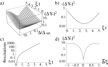
FIG. 6.: (a) Quadrature variance $\Delta Y_{+}^{2}$ vs. single-photon detuning $\Delta$ and interaction time $\xi t$, (b) same for $\Delta=\Delta_{opt}$ and $\delta_{1}=\delta_{2}$ showing maximum squeezing $\Delta Y_{+}^{2}\simeq 0.02$ (for $\sqrt{g^{2}N/\gamma\kappa}=100$), (c) Number of excitations pumped in the system vs. time (same conditions as in b) and (d) $\Delta Y_{+}(t^{*})^{2}$ vs. two-photon detuning ${\bar{\delta}}\equiv(\delta_{1}-\delta_{2})/2$ for $\Delta=\Delta_{opt}$ and where $t^{*}$ gives maximum squeezing.

To quantify the resulting correlations established between the polariton mode $P_{D}$ and the pure spin flip mode $S_{1}$, we introduce the quadratures of both modes (which are bosonic for small number of excitations) in direct analogy to the optical parametric case. We define the quadratures $X_{1}=(S_{1}+S_{1}^{+})/\sqrt{2}$, $Y_{1}=i(S_{1}-S_{1}^{+})/\sqrt{2}$ and similarly for the polarition mode; these can be measured e.g. by converting spin excitations to light. Correlations between the modes appear due to dynamical evolution and squeezing is found in certain quadratures of the sum and difference modes $X_{-}=(X_{1}-X_{D})/\sqrt{2}$ and $Y_{+}=(Y_{1}+Y_{D})\sqrt{2}$. In the language of harmonic oscillators, the positions in mode $1$ and $2=D$ are correlated ($X_{1}\simeq X_{D}$), while the momenta are anti-correlated ($Y_{1}\simeq-Y_{D}$). For small number of excitations the sum and difference modes obey standard commutation relations $\left[X_{\alpha},Y_{\beta}\right]=-i\delta_{\alpha,\beta}$ where $\alpha,\beta=+,-\,{\rm or}\,1,D$. A quadrature $Y_{\pm}$ is squeezed when $\Delta Y_{\pm}(t)^{2}<1/2$ and the Heisenberg limit corresponds to $\Delta Y_{\pm}(t)^{2}\sim 1/N$.

We find that squeezing is optimal under conditions of four-photon resonance ($\delta_{1}=\delta_{2}$) and in the limit of $\eta\gg 1$ (Fig. 6). Evolution leads to squeezing of $Y_{+}$ and $X_{-}$, anti-squeezing of $Y_{-}$ and $X_{+}$. The squeezing in $Y_{+}$ reaches a minimum value at $t=t^{*}$ after which the growing fluctuations in $X_{+}$ give rise to increased noise in $Y_{+}$. Note that the total number of excitations (both modes) in the system, equal to $\langle X_{+}^{2}+X_{-}^{2}+Y_{+}^{2}+Y_{-}^{2}\rangle$, grows exponentially with time (Fig. 6c). Specifically, in the case $g_{1}=g_{2}=g$ and thus $\gamma_{1}=\gamma_{2}\equiv\gamma$, for $\xi t>1$, we have:

$$\left(\Delta Y_{+}(t)\right)^{2} = 1/2\left\{e^{-2\xi t}+\frac{3\gamma_{L}+\kappa/\eta}{2\xi}\right.$$ (64)

$$+ \left.\left(\frac{\gamma_{L}+\kappa/\eta}{2\xi}\right)^{2}e^{2\xi t}\right\}$$ (65)

where we have neglected terms of higher order in $\gamma_{L}/\xi$ and $\kappa/(\eta\xi)$. The maximum amount of squeezing is obtained after an interaction time $t^{*}$ such that $e^{-2\xi t^{*}}=(\gamma_{L}+\kappa/\eta)/2\xi$ and is given by

$$(\Delta Y_{+})^{2}=\frac{5\gamma_{L}+3\kappa/\eta}{4\xi}$$ (66)

i.e. of the order of the damping rate divided by the coherent interaction rate.

Since both the interaction parameter $\xi$ and the relaxation rate of the polariton $\gamma_{D}=\gamma_{L}+\kappa/\eta$ depend on the single photon detuning $\Delta$ (Fig. 6a), we find that squeezing is optimized for

$$\Delta_{opt}=\gamma\sqrt{\frac{5|\Omega_{1}|^{2}}{3|\Omega_{2}|^{2}}\frac{|g|^{2}N}{\gamma\kappa}}$$ (67)

and with this optimal value of the detuning, the squeezing reaches a minimum value of

$$\left(\Delta Y_{+opt}\right)^{2}=\frac{\sqrt{15/4}}{\sqrt{|g|^{2}N/\gamma\kappa}}.$$ (68)

Note that the denominator is equal to the atomic density-length product multiplied by the empty cavity finesse and can easily exceed $10^{4}$ even for modest values of the density-length product and cavity finesse. We further emphasize that typical generation rate resulting in such optimal squeezing $\Omega_{1}\Omega_{2}/\Delta_{opt}$ can easily be on the order of fraction of MHz. In such a case other decoherence mechanisms are negligible. Doppler shifts can also be disregarded as long as all fields are co-propagating.

For the “degenerate” version of the interaction (i.e. with identical final states for the spin flips, see Fig. 4b), the effective hamiltonian can be written as

$$H_{eff}=i\hbar\xi(\hat{S}^{\dagger 2}-\hat{S}^{2})$$ (69)

where the limit $\eta\gg 1$ has been used to write $P_{D}\simeq-S$, with $S=1/\sqrt{N}\Sigma_{gb}$ the spin flip operator. In this case the correlations lead to squeezing of $X=(S+S^{\dagger})/\sqrt{2}$ and anti-squeezing of $Y=i(S-S^{\dagger})/\sqrt{2}$. The analysis for this configuration is very similar to the non-degenerate version, in particular the maximum amount of squeezing achievable is also given by an expression of the form (68).

We can now obtain a condition for achieving Heisenberg-limited spin squeezed states, i.e. $\left(\Delta Y_{+opt}\right)^{2}\simeq 1/N$. We see from (66) that this requires

$$\xi\sim N\Gamma$$ (70)

where $\Gamma=(5\gamma_{L}+4\kappa/\eta)/4$ is the effective damping rate of the system. This is in complete agreement with the estimate based on our simple bosonic model of section III (49). In terms of the single photon Rabi frequency $g$, the cavity decay rate $\kappa$, the spontaneous emission rate $\gamma$ and the number of atoms $N$, the condition for achieving some squeezing i.e. $(\Delta Y_{+})^{2}<1/2$ is

$$|g|^{2}N>\kappa\gamma$$ (71)

which can be easily achieved in the laboratory since it simply corresponds to the condition that the density length product multiplied by the cavity finesse be larger than one. In the cavity QED regime of strong coupling $|g|^{2}\sim\kappa\gamma$, very strong quantum correlations i.e. $(\Delta Y_{+})^{2}\sim 1/\sqrt{N}$ between atoms can be produced. In order to obtain Heisenberg limited spin squeezed states i.e. $(\Delta Y_{+})^{2}\sim 1/N$, one requires a more stringent condition

$$|g|^{2}\sim N\kappa\gamma$$ (72)

which can be fulfilled only in the strong coupling regime of cavity QED for a limited number of atoms. Note that this regime has been achieved experimentally by several groups [30] and would allow for Heisenberg limited spin squeezing for as many as $\sim 10^{3}$ atoms. We have analyzed in this paper the situation of a running-wave cavity, so that all atoms couple equally apart from a possible phase to the cavity mode irrespective of their position. In order to fulfill the cavity QED regime, small cavity volume is needed i.e. standing wave cavities. For atoms in such a cavity the coupling to the cavity mode is position dependent and it becomes necessary to localize atoms accurately at the antinodes of a trapping mode. Note that significant experimental progress has been made towards this direction by several groups [31]. Once the atoms are well localized in the cavity, the interaction can proceed via a neighbouring mode $b$ (e.g. different from the trapping mode $a$) so that for atoms localized within a small region in the cavity the two modes have essentially the same wavelength and atoms would therefore couple equally to the $b$ mode as well, irrespective of their position.

V Discussion and Conclusion

We have reviewed Ramsey spectroscopy and the use of spin squeezed states in precision measurements of this type. With the experimental motivation of minimizing the phase accuracy in phase estimation with Ramsey fringes, we introduced a particular class of squeezed states. These states lead to Heisenberg limited phase accuracy and we developed various pictorial representations for them. The strong similarities of these representations of spin squeezed states to those of squeezed states of light suggests an analogy extending to the type of interaction that gives rise to squeezing. We are thus lead to consider the so-called ”counter twisting” Hamiltonian, which has been shown to lead to maximal spin squeezing. We have studied this model for spin squeezing in the presence of a dissipation mechanism and analyzed the effect of damping and finite system size on the amount of squeezing achievable with such an interaction. The analysis was based on a decorrelation approximation to the BBGKY hierarchy of equations of motion, followed by the use of a linear transformation which in the limit of large number of atoms $1/N\rightarrow 0$ ”contracts” the angular momentum operators onto bosonic operators. This allows for the systematic inclusion of finite system size effects. It appears that Heisenberg limited spin squeezed states may be produced when the single atom nonlinearity exceeds the single atom loss rate. In this case the maximum number of atoms that can be lost before quantum correlations are destroyed to the point of compromising the spin squeezing is of the order $\Delta N\sim\log{N}$. For spin squeezing at a more modest level than the Heisenberg limit, larger number of atoms may be lost without compromising the squeezing, indicating the stronger sensitivity of spin squeezed states to dissipation for larger amounts of squeezing.

We have also presented in detail a scheme based on the interaction of coherent classical light with an optically dense ensemble of atoms that leads to an effective coherent spin-changing interaction involving pairs of atoms. Atoms may be transferred to the same final state leading to spin squeezing (analogous to squeezing of light by degenerate OPO) or to different final states in this case leading to quantum correlations between different atomic modes (analogous to quantum correlations between electromagnetic modes by non-degenerate OPO). We have shown that this process is robust with respect to realistic decoherence mechanisms and can result in rapid generation of correlated (spin squeezed) atomic ensembles. The amount of correlations created by this effective interaction can be simply expressed in terms of the single photon Rabi frequency $g$, the atomic spontaneous emission rate $\gamma$ and the cavity decay rate $\kappa$. We find that the generation of spin squeezed states requires $g^{2}N\sim\kappa\gamma$, which can easily be achieved in low finesse cavities with e.g. room temperature atomic vapours. Very strongly correlated states can be produced when the strong coupling regime $g^{2}\sim\kappa\gamma$ of cavity QED is achieved and the generation of Heisenberg limited spin squeezed states requires $g^{2}\sim N\kappa\gamma$. The effective interaction rate $\xi=\Omega_{1}\Omega_{2}/\Delta$ which depends on the Rabi-frequency of two applied classical fields $\Omega_{1,2}$ and a detuning from an atomic transition $\Delta$ can be fast and is controllable. Furthermore, the resulting spin excitations can be easily converted into photons on demand, which facilitates applications in quantum information processing. Possible applications involving high-precision measurements in atomic clocks can be also foreseen.

We thank M.Fleischhauer, J.I.Cirac, V.Vuletic, S.Yelin and P.Zoller for helpful discussions. This work was supported by the NSF through the grant to the ITAMP.

A Ramsey Spectroscopy

In Ramsey spectroscopy [8], a collection of $N$ two-level atoms are made to interact with two separated fields (in time or in space). The lower and upper states (refered to as ground and excited state) have an energy difference $\hbar\omega_{0}$ and atoms will thus acquire a different dynamical phase $e^{-iEt/\hbar}$ depending on which state they are in. The effect of properly chosen electromagnetic fields is to perform a transformation that prepares the atoms in a superposition of the two states $|g\rangle$ and $|e\rangle$. The different parts of the wavefunction of atoms (corresponding to the ground and excited state) acquire a relative phase due to dynamical evolution and when the inverse transformation is applied, an interference effect is obtained. An exact parallel with the Mach-Zender interferometer can be drawn [32]: the transformation preparing atoms in a superposition of ground and excited states is equivalent to the transformation that lets a photon incident on a beam splitter explore the two arms of an interferometer. The relative phase acquired in the two atomic states during free evolution of duration $T$ is the equivalent of the relative phase acquired by photons travelling in the arms of the interferometer. Finally, the second pulse that performs the inverse transformation on atoms is the equivalent of the recombination of signals from the two interferometer arms on a beam splitter. At the end of this sequence, the number of atoms in either states, equivalent to the number of photons from either output of the final beam splitter, is measured. In this way, the signal measured depends on the acquired relative phase which can thus be estimated with some accuracy.

We will now quantify this more precisely: let the frequency of the applied electromagnetic pulses be $\omega$, and the time delay between the two zones of interaction be $T$. The duration and strength of the applied fields are chosen so as to lead to $\pi/2$ pulses, i.e. transformation of the atomic state according to

$$|e\rangle \rightarrow \frac{|e\rangle-i|g\rangle}{\sqrt{2}}$$ (A1)

$$|g\rangle \rightarrow \frac{|e\rangle+i|g\rangle}{\sqrt{2}}.$$ (A2)

During their free evolution between the two zones, atoms in the ground and excited states acquire a relative phase $\phi$ which, in a frame rotating with the frequency of the applied field, is $\phi=(\omega-\omega_{0})T$.

Before entering the first interaction zone, the atoms are prepared in their lower state $|g\rangle$ and at the exit of the second zone, the number of atoms in states $|e\rangle$ and $|g\rangle$ is measured.

For simplicity, we consider the case when the first zone leads to a $\pi/2$ pulse and the second one a $-\pi/2$ pulse. The picture of angular momentum is particularly well suited to discuss the Ramsey interferometric scheme and leads to an intuitive pictorial representation of the scheme. The Schwinger angular momentum operators are defined as

$$\hat{J}_{x} = (\hat{\Sigma}_{eg}+\hat{\Sigma}_{ge})/2$$ (A3)

$$\hat{J}_{y} = (\hat{\Sigma}_{eg}-\hat{\Sigma}_{ge})/2i$$ (A4)

$$\hat{J}_{z} = (\hat{\Sigma}_{ee}-\hat{\Sigma}_{gg})/2$$ (A5)

where $\hat{\Sigma}_{\mu\nu}=\sum_{j=1}^{N}|\mu\rangle_{jj}\langle\nu|$ are collective operators. In terms of these, a single $\pi/2$ pulse (A2) is represented by a rotation of the pseudo angular momentum vector around the x-axis by an angle $\pi/2$. For a single atom we have the correspondence $|\uparrow\rangle=|e\rangle$ and $|\downarrow\rangle=|g\rangle$. Under a $\pi/2$ rotation about the x-axis, the state $\uparrow\rangle$ transforms to $|J_{y}=-1/2\rangle=(|\uparrow\rangle-i|\downarrow\rangle)/\sqrt{2}$ as indicated in (A2). For $N$ atoms, we can think of the $N$ individual spin ${\frac{1}{2}}$ particles combining to form a pseudo angular momentum vector of length $J=N/2$. The state of the collection of $N$ atoms can then be represented by appropriate superpositions of the states $|J,M\rangle$ where $-J\leq M\leq J$. Of course, only states within the completely symmetric subspace of the full $2^{N}$-dimensional Hilbert space can be represented in this way, which is justified since the coherent interaction of the electromagnetic fields with the atoms couple only to this symmetric subspace (i.e. all atoms couple equally to the fields).

Free evolution in the rotating frame corresponds to rotation of the angular momentum around the z-axis at an angular velocity $\omega-\omega_{0}$. The whole Ramsey scheme can then be represented by the sequence: $\pi/2$ rotation about x-axis, $\phi$ rotation about the z-axis and $-\pi/2$ rotation about the x-axis. This is the transformation perfomed by the unitary operator

$$\hat{U}(\phi)=e^{i\pi/2\hat{J}_{x}}e^{-i\phi\hat{J}_{z}}e^{-i\pi/2\hat{J}_{x}}$$ (A6)

where $\phi=(\omega-\omega_{0})T$ as before. At the end of the scheme, the number of atoms in states $|e\rangle$ and $|g\rangle$ is measured, or equivalently their difference $\hat{J}_{z}(\phi)$ where

$$\hat{J}_{z}(\phi) = \hat{U}(\phi)^{\dagger}\hat{J}_{z}\hat{U}(\phi)$$ (A7)

$$= \hat{J}_{z}\cos\phi-\hat{J}_{x}\sin\phi.$$ (A8)

The Ramsey signal is thus

$$\langle\hat{J}_{z}(\phi)\rangle=\langle\hat{J}_{z}\rangle\cos\phi-\langle\hat{J}_{x}\rangle\sin\phi$$ (A9)

and its variance $\Delta J_{z}(\phi)$ is

$$\Delta J_{z}(\phi) = \left[(\Delta J_{z})^{2}\cos^{2}\phi+(\Delta J_{x})^{2}\sin^{2}\phi\right.$$ (A10)

$$- \left.\cos\phi\sin\phi(\langle\hat{J}_{x}\hat{J}_{z}+\hat{J}_{z}\hat{J}_{x}\rangle-2\langle\hat{J}_{z}\rangle\langle\hat{J}_{x}\rangle)\right]^{1/2}$$ (A11)

where the variance is defined as $(\Delta A)^{2}=\langle\hat{A}^{2}\rangle-\langle\hat{A}\rangle^{2}$. From the signal one wants to estimate the phase $\phi$ and thus the frequency difference $\omega-\omega_{0}$. The phase accuracy achievable from such a measurement is related to the signal variance (the “noise”) by

$$\delta\phi(\phi)=\frac{\Delta J_{z}(\phi)}{|\frac{\partial\langle\hat{J}_{z}(\phi)\rangle}{\partial\phi}|}.$$ (A12)

For states such that $\langle\hat{J}_{x}\rangle=0$ (all the states we will consider in this paper are of this type), the sensitivity $|\partial\langle\hat{J}_{z}(\phi)\rangle/\partial\phi|$ is maximal for $\phi=\pm\pi/2$ and the phase accuracy can be expressed as

$$\delta\phi(\pm\pi/2)=\frac{\Delta J_{x}}{|\langle\hat{J}_{z}\rangle|}.$$ (A13)

Since $\Delta J_{x}$ and $\langle\hat{J}_{z}\rangle$ depend on the initial state, we see that different initial states lead to different phase accuracies. Of particular importance is the accuracy achievable when all atoms are prepared in the same initial state. In this case the state of the atomic ensemble is a pure state, but it is however an uncorrelated state of the atomic ensemble (i.e. it can be factorized $|\Psi\rangle=\prod_{j=1}^{N}|\psi\rangle_{j}$).

Consider the case of uncorrelated atoms for which all atoms have been prepared in the lower state $|g\rangle$, sometimes called a Bloch state. The state of the atomic ensemble can thus be expressed in terms of eigenstates of the collective angular momentum operators as

$$\prod_{j=1}^{N}|g\rangle_{j}=|J=N/2,J_{z}=-N/2\rangle$$ (A14)

where $J=N/2$ since there are $N$ $2$-level atoms, equivalent to $N$ spin ${\frac{1}{2}}$ particles. For such a state, the expectation value of the angular momentum operators and their variances are calculated to be $\langle\hat{J}_{x}\rangle=\langle\hat{J}_{y}\rangle=0$, $\langle\hat{J}_{z}\rangle=-J$, $\Delta J_{x}=\Delta J_{y}=\sqrt{J/2}$ and $\Delta J_{z}=0$. The signal and its variance are thus

$$\langle\hat{J}_{z}(\phi)\rangle = -J\cos\phi$$ (A15)

$$\Delta J_{z}(\phi) = \sqrt{J/2}\sin\phi.$$ (A16)

The maximum sensitivity is achieved at $\phi=\pm\pi/2$

$$\delta\phi(\pm\pi/2)=\frac{1}{\sqrt{2J}}=\frac{1}{\sqrt{N}}$$ (A17)

which is the standard quantum limit (SQL). Performing the experiment on $N$ independent atoms all prepared in the same initial state is thus equivalent to repeating the experiment on one atom $N$ times and leads to an expected $1/\sqrt{N}$ factor of improvement in accuracy over the one atom result $\Delta S_{x}/\langle\hat{S}_{z}\rangle=1$. This is the best accuracy achievable with atoms all prepared in the same initial pure quantum state. The number of atoms detected in the upper state, given by $\langle\hat{N}_{+}(\phi)\rangle=N/2+\langle\hat{J}_{z}(\phi)\rangle$, and its variance are shown in Fig.1a.

There is a lower bound on the phase accuracy, set by Heisenberg’s uncertainty principle, $\Delta J_{i}\Delta J_{j}\geq{\frac{1}{2}}|\langle[\hat{J}_{i},\hat{J}_{j}]\rangle|$ where $i,j=x,y,z$. It is straightforward to show that

$$\delta\phi\geq\frac{1}{N}$$ (A18)

which is known as the Heisenberg limit.

We now see from (A13) that in order to surpass the SQL, the atomic ensemble must be prepared in a state such that $\Delta J_{x}/|\langle J_{z}\rangle|\leq 1/\sqrt{N}$, which is a necessary and sufficient condition for entanglement of an atomic ensemble [23]. It is thus important to have a state for which the variance $\Delta J_{x}$ is reduced compared to its value for the uncorrelated state (A14) while maintaining a large value for $\langle J_{z}\rangle$ so that the amplitude of the signal $\langle\hat{J}_{z}(\phi)\rangle=\langle\hat{J}_{z}\rangle\cos\phi$ is not compromised [20]. Such states which have reduced uncertainty in one observable $\Delta J_{x}$ (at the expense of the conjugate observable $\Delta J_{y}$ having increased fluctuations) have been called spin-squeezed states [5].

B Spin squeezed states - Wigner function representation

We now consider the Wigner function representation of the states $|\psi(a)\rangle$. The Wigner distribution of general angular-momentum states [33] is obtained from an expansion of the density operator in terms of the multipole operators

$$\hat{\rho}=\sum_{k=0}^{2J}\sum_{q=-k}^{+k}\rho_{kq}\hat{T}_{kq}$$ (B1)

where the multipole operators are

$$\hat{T}_{kq} = \sum_{m=-J}^{+J}\sum_{m^{\prime}=-J}^{+J}(-1)^{J-m}\sqrt{2k+1}\left(\begin{array}[]{ccc}J&k&J\\ -m&q&m^{\prime}\end{array}\right)$$ (B4)

$$\times |J,m\rangle\langle J,m^{\prime}|$$ (B5)

and $\left(\begin{array}[]{ccc}J&k&J\\ -m&q&m^{\prime}\end{array}\right)$ is the usual Wigner $3j$ symbol. The wigner distribution is then given by

$$W(\theta,\phi) = \sum_{k=0}^{2J}\sum_{q=-k}^{+k}Y_{k}^{q}(\theta,\phi)\rho_{kq}$$ (B6)

where $\rho_{kq}=\langle\hat{T}_{kq}\rangle={\rm Tr}[\hat{\rho}\hat{T}_{kq}]$ and $Y_{k}^{q}(\theta,\phi)$ are the spherical harmonics. In Fig. 7, the Wigner function for the state $|\psi(-1)\rangle$ clearly shows the way in which this state has a large negative expectation value for $\hat{J}_{z}$, reduced variance in $\hat{J}_{x}$ and increased variance in $\hat{J}_{y}$.

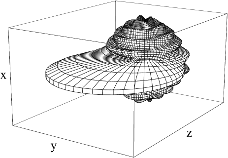
FIG. 7.: Wigner function representation of the state $|\psi(a)\rangle$ with $a=-1)$. Plotted is the surface $r(\theta,\phi)=W(\theta,\phi)$, showing the large and negative value of $\langle\hat{J}_{z}\rangle$, reduced variance $\Delta J_{x}$ and correspondingly increased variance $\Delta J_{y}$.

C Adiabatic elimination of excited state in Raman scattering

From the Hamitonian (51), we obtain the equations of motion for the cavity mode and the ground state coherence $\Sigma_{gb_{1}}$

$$\dot{a} = -\kappa a-ig_{1}^{*}\Sigma_{b_{1}a_{1}}-ig_{2}^{*}\Sigma_{ga_{2}}+F_{a}(t)$$ (C1)

$$\dot{\Sigma}_{gb_{1}} = -(\gamma_{0}-i\delta_{1})\Sigma_{gb_{1}}+i\Omega_{1}\Sigma_{a_{1}b_{1}}-ig_{1}^{*}a^{\dagger}\Sigma_{ga_{1}}$$ (C2)

$$+ F_{gb_{1}}(t)$$ (C3)

and the optical polarizations associated with Stokes emission evolve according to

$$\dot{\Sigma}_{b_{1}a_{1}} = -[\gamma-i(\Delta-\delta_{1})]\Sigma_{b_{1}a_{1}}-i\Omega_{1}\Sigma_{b_{1}g}$$ (C4)

$$- ig_{1}a(\Sigma_{b_{1}b_{1}}-\Sigma_{a_{1}a_{1}})+F_{b_{1}a_{1}}(t)$$ (C5)

$$\dot{\Sigma}_{a_{1}g} = -(\gamma+i\Delta)\Sigma_{a_{1}g}-i\Omega_{1}^{*}(\Sigma_{a_{1}a_{1}}-\Sigma_{gg})$$ (C6)

$$+ ig_{1}^{*}a^{\dagger}\Sigma_{b_{1}g}+F_{a_{1}g}(t)$$ (C7)

where we assume that population in the excited state $|a_{1}\rangle$ decays towards $|b_{1}\rangle$ at a rate $\gamma_{1}$, towards $|g\rangle$ at a rate $\gamma_{2}$ and we assume a dephasing rate $\gamma_{0}$ for ground state coherences ($\gamma=(\gamma_{1}+\gamma_{2})/2$ and $\gamma\gg\gamma_{0}$).

We proceed by adiabatic elimination of optical polarizations associated with Stokes emission. To this end we assume large single-photon detuning $\Delta\gg\gamma$ and to first order in $\hat{a}$ we obtain ($\Sigma_{gg}\sim N$)

$$\Sigma_{b_{1}a_{1}} = \frac{\Omega_{1}}{\Delta}(1-i\frac{\gamma}{\Delta})\Sigma_{b_{1}g}+i\frac{F_{b_{1}a_{1}}(t)}{\Delta}$$ (C8)

$$\Sigma_{a_{1}g} = \frac{\Omega_{1}^{*}}{\Delta}N(1+i\frac{\gamma}{\Delta})-i\frac{F_{a_{1}g}(t)}{\Delta}$$ (C9)

which we substitute in (C3) and obtain for the ground state spin flip operator $S_{1}=\Sigma_{gb_{1}}/\sqrt{N}$

$$\dot{S_{1}} = -\left[(\gamma_{0}+\gamma_{L})-i(\delta_{1}+\delta_{L})\right]S_{1}-i\frac{g_{1}^{*}\sqrt{N}\Omega_{1}}{\Delta}a^{\dagger}$$ (C10)

$$+ {\bar{F}}_{S_{1}}(t)$$ (C11)

where $\gamma_{L}=\gamma|\Omega_{1}|^{2}/\Delta^{2}$ is an optical pumping rate, $\delta_{L}=|\Omega_{1}|^{2}/\Delta$ is the light shift and ${\bar{F}}_{S_{1}}(t)$ is a modified noise force. Light shifts can be incorporated in a redefinition of the energies and we ignore them in the remainder of this paper. Since the ground state decoherence rate is typically very small, we also assume $\gamma_{L}\gg\gamma_{0}$ and in that limit the new $\delta$-correlated noise forces have correlations

$$\langle{\bar{F}}_{S_{1}}(t){\bar{F}}_{S_{1}}^{\dagger}(t^{\prime})\rangle = 2\gamma_{L}\frac{\gamma_{2}}{\gamma}\delta(t-t^{\prime})$$ (C12)

$$\langle{\bar{F}}_{S_{1}}^{\dagger}(t){\bar{F}}_{S_{1}}(t^{\prime})\rangle = 2\gamma_{L}\frac{\gamma_{1}}{\gamma}\delta(t-t^{\prime})$$ (C13)

D Adiabatic elimination of bright polariton

After adiabatic elimination of the excited state $|a_{1}\rangle$, the relevant equations of motion are

$$\dot{S}_{1}^{\dagger} = -(\gamma_{L}+i\delta_{1})S_{1}^{\dagger}+i\chi a+{\bar{F}}_{S_{1}}^{\dagger}(t)$$ (D1)

$$\dot{a} = -\kappa a-i\chi^{*}S_{1}^{\dagger}-ig_{2}^{*}\Sigma_{ga_{2}}+F_{a}(t)$$ (D2)

$$\dot{S}_{2} = -(\gamma_{L}+i\delta_{2})S_{2}-i\frac{\Omega_{2}^{*}}{\sqrt{N}}\Sigma_{ga_{2}}+{\bar{F}}_{S_{2}}(t)$$ (D3)

$$\dot{\Sigma}_{ga_{2}} = -(\gamma+i\delta_{2})\Sigma_{ga_{2}}-i\Omega_{2}\sqrt{N}S_{2}-ig_{2}Na$$ (D4)

$$+ F_{ga_{2}}(t)$$ (D5)

where $S_{2}=\Sigma_{gb_{2}}/\sqrt{N}$.

From (D5) and (57) and in the limit of large ratio of speed of light in vacuum to group velocity of Stokes photons $\eta=|g_{2}|^{2}N/|\Omega_{2}|^{2}\gg 1$, we obtain the equations of motion in terms of bright and dark polaritons

$$\dot{S}_{1}^{\dagger} = -(\gamma_{L}+i\delta_{1})S_{1}^{\dagger}+i\chi(\frac{P_{D}}{\eta}+P_{B})+F_{S_{1}}^{\dagger}(t)$$ (D6)

$$\dot{P}_{D} = -(\kappa/\eta+\Gamma_{2})P_{D}-i\frac{\chi^{*}}{\sqrt{\eta}}S_{1}^{\dagger}-\frac{\kappa-\Gamma_{2}}{\sqrt{\eta}}P_{B}$$ (D7)

$$+ F_{D}(t)$$ (D8)

$$\dot{P}_{B} = -(\kappa+\Gamma_{2}/\eta)P_{B}-i\chi^{*}S_{1}^{\dagger}-ig_{2}\sqrt{N}{\tilde{\Sigma}}_{ga_{2}}$$ (D9)

$$+ F_{B}(t)$$ (D10)

$$\dot{{\tilde{\Sigma}}}_{ga_{2}} = -\Gamma{\tilde{\Sigma}}_{ga_{2}}-ig_{2}\sqrt{N}P_{B}+{\tilde{F}}_{ga_{2}}(t)$$ (D11)

where $\Gamma_{2}=\gamma_{L}+i\delta_{2}$, $\Gamma=\gamma+i\delta_{2}$ and ${\tilde{\Sigma}}_{ga_{2}}=\Sigma_{ga_{2}}/\sqrt{N}$ and noise forces were modified appropriately. Note that in the picture of dark and bright polaritons, only the bright polariton is coupled to the excited state through the optical coherence $\Sigma_{ga_{2}}$.

Under adiabatic conditions, the bright polariton evolves slowly (on a typical timescale $T$) and we can solve perturbatively in $1/T$. The equations (D10) and (D11) are of the form $\dot{{\bf x}}=-{\bf M}.{\bf x}+{\bf y}$, where ${\bf x}$ is the vector $(P_{B},{\tilde{\Sigma}}_{ga_{2}})$, ${\bf M}$ is a $2\times 2$ matrix and ${\bf y}$ is a source term

$$\frac{d}{dt}\left[\begin{array}[]{c}P_{B}\\ {\tilde{\Sigma}}_{ga_{2}}\end{array}\right] = -\left(\begin{array}[]{cc}\kappa&ig_{2}\sqrt{N}\\ ig_{2}\sqrt{N}&\Gamma\end{array}\right)\left[\begin{array}[]{c}P_{B}\\ {\tilde{\Sigma}}_{ga_{2}}\end{array}\right]$$ (D18)

$$+ \left[\begin{array}[]{c}-i\chi^{*}S_{1}^{\dagger}-\frac{\kappa}{\eta}P_{D}+F_{B}(t)\\ {\tilde{F}}_{ga_{2}}(t)\end{array}\right]$$ (D21)

where we have used $\kappa\gg\gamma_{L}$ and where $F_{B}(t)$ and ${\tilde{F}}_{ga_{2}}(t)$ are appropriate noise forces. These equations can be solved easily to first order by ${\bf x}^{(0)}(t)={\bf M}^{-1}.{\bf y}$, higher order approximations yielding ${\bf x}^{(n)}(t)={\bf M}^{-1}.[{\bf y}-\dot{{\bf x}}^{(n-1)}(t)]$.

We can rewrite

$$\frac{|g_{2}|^{2}N}{\kappa\gamma}\sim 3\pi\times\left(\frac{N}{V}L\lambda^{2}\right)\times{\mathcal{F}}$$ (D22)

i.e. the density length product multiplied by the cavity finesse, so that with densities corresponding to room temperature atomic vapours, optical wavelengths and finesse of order $100$ this quantity is already of order $\sim 10^{4}$. We can thus assume that $|g_{2}|^{2}N/(\kappa\gamma)\gg 1$ and solve in powers of $\kappa\gamma/(|g_{2}|^{2}N)$.

We see from (D21) that ${\bf x}^{(n)}(t)$ is of order $[\kappa\gamma/(|g_{2}|^{2}N)]^{(n+1)}$ and thus solving to lowest order we find

$$P_{B} = \frac{1}{|g_{2}|^{2}N}[-i\Gamma\chi^{*}S_{1}^{\dagger}-\frac{\kappa\Gamma}{\sqrt{\eta}}P_{D}+\Gamma F_{B}(t)$$ (D23)

$$- ig_{2}F_{ga_{2}}(t)]$$ (D24)

so that when $\eta\gg 1$,

$$a \simeq \frac{P_{D}}{\eta}+P_{B}$$ (D25)

$$\simeq \frac{P_{D}}{\eta}+\frac{1}{|g_{2}|^{2}N}[-i\Gamma\chi^{*}S_{1}^{\dagger}+\Gamma F_{B}(t)$$ (D26)

$$- ig_{2}F_{ga_{2}}(t)].$$ (D27)

The coupled equations of motion for the dark state polariton (D8) and the spin flip (D6) then become

$$\dot{S}_{1}^{\dagger} = (\frac{|g_{1}|^{2}}{|g_{2}|^{2}}\gamma_{L}-\gamma_{L}-i\delta_{1})S_{1}^{\dagger}+i\frac{\chi}{\sqrt{\eta}}P_{D}+{\tilde{F}}_{S_{1}}^{\dagger}(t)$$ (D28)

$$\dot{P}_{D} = -(\kappa/\eta+\gamma_{L}+i\delta_{2})P_{D}-i\frac{\chi^{*}}{\sqrt{\eta}}S_{1}^{\dagger}+{\tilde{F}}_{D}(t)$$ (D29)

where ${\tilde{F}}_{S_{1}}^{\dagger}(t)$ and ${\tilde{F}}_{D}(t)$ are modified noise forces with correlations

$$\langle{\tilde{F}}_{D}(t){\tilde{F}}_{D}^{\dagger}(t^{\prime})\rangle = \frac{\kappa}{\eta}+2\gamma_{L}\frac{\gamma_{2}}{\gamma}$$ (D30)

$$\langle{\tilde{F}}_{D}^{\dagger}(t){\tilde{F}}_{D}(t^{\prime})\rangle = 2\gamma_{L}\frac{\gamma_{1}}{\gamma}$$ (D31)

$$\langle{\tilde{F}}_{S_{1}}(t){\tilde{F}}_{S_{1}}^{\dagger}(t^{\prime})\rangle = 2\gamma_{L}\frac{\gamma_{2}}{\gamma}$$ (D32)

$$\langle{\tilde{F}}_{S_{1}}^{\dagger}(t){\tilde{F}}_{S_{1}}(t^{\prime})\rangle = 2\gamma_{L}\frac{\gamma_{1}}{\gamma}$$ (D33)

and all other correlations can be neglected. The coherent part of the interaction can thus be obtained from an effective hamiltonian

$$H_{eff}=\frac{\hbar\chi}{\sqrt{\eta}}S_{1}P_{D}+{\rm h.c.}$$ (D35)

where the interaction rate is $\chi/\sqrt{\eta}=g_{1}\Omega_{1}^{*}|\Omega_{2}|/(|g_{2}|\Delta)$.

We note (D29) that cavity losses are strongly suppressed in the limit $\eta\gg 1$. Indeed, subsequent to the large group velocity reduction [15], the polariton is almost purely atomic and the excitation leaks very slowly out of the medium. The equation of motion for coherence $S_{1}^{+}$ (D28) contains a loss term (due to isotropic spontaneous emission) and a linear gain term (due to emission into bright polariton). The two can compensate each other. However the linear phase-insensitive amplification is also accompanied by correspondingly increased fluctuations, represented by new Langevin forces $\tilde{F}_{D}(t),\tilde{F}_{S_{1}}^{+}(t)$. In the case that $g_{1}=g_{2}$ and when all Rabi frequencies are taken to be real, we have the interaction rate $\xi=\chi/\sqrt{\eta}=\Omega_{1}\Omega_{2}/\Delta$.

REFERENCES

- [1] H.J. Kimble, in Fundamental systems in quantum optics, edited by J. Dalibard, J.-M. Raimond and J. Zinn-Justin (North-Holland 1990).
- [2] D.F. Walls and G.J. Milburn, Quantum Optics (Springer, Berlin, 1994).
- [3] K. Mattle et al., Phys. Rev. Lett. 76 4656, (1996); Z.Y.Ou et. al, Phys. Rev. Lett. 68 3663 (1992)
- [4] L.-M. Duan, M.D. Lukin, J.I. Cirac and P. Zoller, quant-ph/0105105.
- [5] M. Kitagawa and M. Ueda, Phys. Rev. A 47, 5138 (1993).
- [6] D. Bouwmeester, A.K. Ekert, A. Zeilinger (eds.), The physics of quantum information, (Springer , New York, 2000).
- [7] M.A. Nielsen and I.L. Chuang., Quantum computation and quantum information, (Cambridge University Press, New York, 2000).
- [8] D.J. Wineland, et al., Phys. Rev. A 46, R6797 (1992); ibid 50, 67 (1994); J.J. Bollinger et al. Phys. Rev. A 54 R4649 (1996); S. F. Huelga et al. Phys. Rev. Lett. 79, 3865 (1997); V. Meyer et al., Phys. Rev. Lett. 86 5870 (2001).
- [9] S.Sachdev, Quantum phase transitions, (Cambridge University Press, New York, 1999).
- [10] C.A. Sackett et al., Nature 404, 256 (2000).
- [11] B. Julsgaard, A. Kozhekin and E. Polzik, Nature 413 400 (2001).
- [12] H. Touchette and S. Lloyd, Phys. Rev. Lett. 84, 1156 (2000).
- [13] P.Meystre, Atom Optics, (Springer , New York, 2001).
- [14] A. André, L.-M. Duan and M.D. Lukin, quant-ph/0107075
- [15] L. V. Hau et al., Nature 397, 594 (1999); M. Kash et al. Phys. Rev. Lett. 82, 5229 (1999); D. Budker et al., Phys. Rev. Lett. 83, 1767 (1999).
- [16] C. Liu, Z. Dutton, C.H. Behroozi and L. Hau, Nature 409, 490 (2001); D.F. Phillips et al., Phys. Rev. Lett. 86, 783 (2001).
- [17] M.D. Lukin, S.F. Yelin and M. Fleischhauer, Phys. Rev. Lett. 84, 4232 (2000); M. Fleischhauer and M.D. Lukin, Phys. Rev. Lett. 84, 5094 (2000).
- [18] J.I. Cirac, P. Zoller, H.J. Kimble and H. Mabuchi, Phys. Rev. Lett. 78, 3221 (1997); S.J. Enk, J.I. Cirac and P. Zoller, Science 279, 205 (1998).
- [19] P. Bouyer and M.A. Kasevich, Phys. Rev. A 56 R1083 (1997).
- [20] T. Kim et al. Phys. Rev. A 57, 4004 (1998).
- [21] J.R. Anglin and A. Vardi, Phys. Rev. A 64, 013605 (2001)
- [22] F.T. Arecchi et al., Phys. Rev. A 6 2211 (1972).
- [23] L.-M. Duan, A. Sørensen, J. I. Cirac and P. Zoller Phys. Rev. Lett. 85, 3991 (2000); A. Sørensen, L.-M. Duan, J. I. Cirac and P. Zoller, Nature 409,63 (2001).
- [24] A. Kuzmich, K. Mølmer, and E. S. Polzik, Phys. Rev. Lett. 79, 4782 (1997); J. Hald, et al., ibid 1319 (1999).
- [25] A. Kuzmich, L. Mandel and N.P. Bigelow, Phys. Rev. Lett. 85, 1594 (2000).
- [26] I. Bouchoule and K. Mølmer, quant-ph/0105144
- [27] M. Fleischhauer and M.D. Lukin, quant-ph/0106066
- [28] J. Stenger et al., Nature 396, 345 (1998).
- [29] D.J. Heinzen, R. Wynar, P.D. Drummond and K.V. Kheruntsyan, Phys. Rev. Lett. 84, 5029 (2000).
- [30] P.W.H. Pinkse et al., J. Mod. Opt. 47, 2769 (2000); C.J. Hood et al., Phys. Rev. A 64, 033804 (2001).
- [31] J. Ye et al., Phys. Rev. Lett. 83, 4987 (1999); P.W.H. Pinkse et al., Nature 404, 365 (2000).
- [32] J.P. Dowling, Phys. Rev. A 57 4736 (1998).
- [33] J.P. Dowling, G.S. Agarwal and W.P. Schleich, Phys. Rev. A 49, 4101 (1994).