Quadrature–dependent Bogoliubov transformations
and multiphoton squeezed states

Abstract

We introduce a linear, canonical transformation of the fundamental single–mode field operators $a$ and $a^{\dagger}$ that generalizes the linear Bogoliubov transformation familiar in the construction of the harmonic oscillator squeezed states. This generalization is obtained by adding to the linear transformation a nonlinear function of any of the fundamental quadrature operators $X_{1}$ and $X_{2}$, making the original Bogoliubov transformation quadrature–dependent. Remarkably, the conditions of canonicity do not impose any constraint on the form of the nonlinear function, and lead to a set of nontrivial algebraic relations between the $c$–number coefficients of the transformation. We examine in detail the structure and the properties of the new quantum states defined as eigenvectors of the transformed annihilation operator $b$. These eigenvectors define a class of multiphoton squeezed states. The structure of the uncertainty products and of the quasiprobability distributions in phase space shows that besides coherence properties, these states exhibit a squeezing and a deformation (cooling) of the phase–space trajectories, both of which strongly depend on the form of the nonlinear function. The presence of the extra nonlinear term in the phase of the wave functions has also relevant consequences on photon statistics and correlation properties. The non quadratic structure of the associated Hamiltonians suggests that these states be generated in connection with multiphoton processes in media with higher nonlinearities.

PACS. 03.65.Sq, 42.50.Dv.

I Introduction

The generalization of the squeezed states of the harmonic oscillator to different systems and the definition of new nonclassical states of light have been actively pursued in recent years [1], [2], [3] [4], [5], [6], [7]. The possibility of experimental realization has also been discussed in some instances [8], [9], [10]. However, these proposed generalizations cannot be easily and straightforwardly connected to canonical and Hamiltonian structures. Generalizations providing a Hamiltonian structure and at the same time preserving the canonical commutation relations would thus be extremely desirable not only from a mathematical and conceptual point of view, but expecially for possible connections to new physical systems and experimental realizations.

In this paper we present a natural generalization of the Bogoliubov transformation originally introduced by Yuen to define the two–photon coherent states of the harmonic oscillator [11]. This generalization is achieved by simply adding to the original transformation, which is linear in the fundamental mode variables $a$ and $a^{\dagger}$, a nonlinear operator–valued function $F(X_{i})$ of any of the fundamental quadratures $X_{1}$ and $X_{2}$. The nonlinear function $F$ is by definition hermitian, and thus defines a quadrature–dependent Bogoliubov transformation. The transformed modes $b$ and $b^{\dagger}$ obey the canonical commutation relations $[b,b^{\dagger}]$ under suitable constraints on the coefficients of the transformation. Such constraints are in fact broad enough to allow for enough freedom on the variation of the coefficients. The eigenvectors of the transformed annihilation operator $b$ define the quadrature–dependent generalization of the squeezed states of the harmonic oscillator. Such states are thus multiphoton squeezed states associated to non quadratic Hamiltonian systems. They preserve some coherence properties, such as the classical motion of the wave–packet center, but in addition they exhibit nonclassical features such as amplitude squeezing, interference and deformation in phase space, super–Poissonian modifications of the field statistics and of the second–order correlation functions. To avoid possible sources of confusion, we emphasize that the multiphoton squeezed states defined in the present work should not be confused with the nonlinear coherent states defined in the literature [10] as the eigenstates of nonlinear operator valued functions of the number operator. In fact, both the physical origin and the mathematical properties of these two classes of states are rather different; they are both associated to multiphoton down conversion processes, but the multiphoton squeezed states are generated in multiphoton down conversion processes in optical parametric amplifiers of higher $\chi$ nonlinearity, while the nonlinear coherent states are produced in multiphoton down conversion processes in the quantized motion of a trapped atom (the counterpart of this process has also been recently studied [12]).

The plan of the paper is the following: the quadrature–dependent Bogoliubov transformation is introduced in Sec. II, and the conditions of canonicity are discussed. In Sec. III we introduce and discuss in some detail the Hamiltonian structure induced by the transformation; in particular, we provide the explicit form of the Hamiltonian expressed in terms of the original mode variables for the lowest nonlinear function of the amplitude $F(X_{1})=X_{1}^{2}$. The properties of the uncertainty products are studied in Sec. IV, where it is shown that the multiphoton squeezed states associated to the quadrature–dependent Bogoliubov transformation exhibit amplitude squeezing and are moreover asymptotically of minimum uncertainty. The eigenvalue equation defining the multiphoton squeezed states are explicitly solved in the quadrature representation in Sec. V, and the coherent motion of the wave–packet center is obtained. Results for the photon number distributions and second–order correlation functions are presented in Sec. VI, while in Sec. VII we perform the phase–space analysis of the multiphoton squeezed states in terms of the Wigner quasiprobability distributions and of the classical parametric trajectories. Comments and conclusions follow in Sec. VIII.

II The Quadrature–dependent Bogoliubov Transformation

Let us consider a single–mode bosonic quantum system. The fundamental adimensional variables are the bosonic annihilation and creation operators $a$ and $a^{\dagger}$, with canonical commutation relation $[a,a^{\dagger}]=1$.

We introduce a new set of fundamental variables $b$ and $b^{\dagger}$ by the linear transformation

$$b=\mu a+\nu a^{\dagger}+\gamma F(X_{1})+\eta G(X_{2})\;,$$ (1)

and its adjoint

$$b^{\dagger}=\mu^{*}a^{\dagger}+\nu^{*}a+\gamma^{*}F(X_{1})+\eta^{*}G(X_{2})\;.$$ (2)

In the above, $\mu$, $\nu$, and $\gamma$ are complex numbers, while $F=F^{\dagger}$ and $G=G^{\dagger}$ are operator–valued nonlinear functions of the fundamental quadrature operators

$$X_{1}=\frac{a+a^{\dagger}}{2}\,,\;\;\;\;\;\;\;\;\;\;X_{2}=\frac{a-a^{\dagger}}{2i}\;.$$ (3)

The transformation is obviously a linear mapping in the space of operators. On the other hand, it is in general a nonlinear, quadrature–dependent extension of the Bogoliubov transformation in the sense that the latter is recovered either if $\gamma=\eta=0$, or if $F$ and $G$ contain only linear powers of the quadratures.

To begin with, we will study, for simplicity, only the quadrature–dependent Bogoliubov transformation generated by the first quadrature $X_{1}$ alone, i.e. we put $\eta=0$ in Eqs. (1) and (2) and thus consider the transformation

$$b=\mu a+\nu a^{\dagger}+\gamma F(X_{1})\;,$$ (4)

together with its adjoint

$$b^{\dagger}=\mu^{*}a^{\dagger}+\nu^{*}a+\gamma^{*}F(X_{1})\;.$$ (5)

In fact, all the main features of the quantum states generated by the quadrature–dependent Bogoliubov transformations are already contained in this instance. The extension to transformations generated by $G(X_{2})$ alone, and by both $F(X_{1})$ and $G(X_{2})$ will be briefly discussed in the conclusions.

i) Canonical structure. We first analyze under what conditions the quadrature–dependent Bogoliubov transformation (4)–(5) is canonical. With a little algebra, we have that $[b,b^{\dagger}]=1$ if

$$|\mu|^{2}-|\nu|^{2} = 1\;,$$ (6)

$${\mathrm{Re}}(\mu\gamma^{*}-\nu^{*}\gamma) = 0\;,$$ (8)

where ${\mathrm{Re}}(z)$ denotes the real part of the complex number $z$. It is a remarkable feature that the conditions of canonicity for the quadrature–dependent Bogoliubov transformation are relations for the $c$–number coefficients of the transformation only, and do not involve the operator–valued function $F(X_{1})$. The same is true also when considering the quadrature–dependent Bogoliubov transformations generated by $G(X_{2})$ alone, or by both $F(X_{1})$ and $G(X_{2})$. Therefore, the form of the operator–valued functions $F(X_{1})$ and $G(X_{2})$ is not constrained by requiring the transformation to be canonical.

The relations (6) are such to give enough freedom in the choice of the coefficients of the transformation. This would not be true if we had attempted to generalize the linear Bogoliubov transformation introducing nonlinear operator–valued functions $A(a)$ and/or $B(a^{\dagger})$ of the fundamental mode variables rather than of the quadratures. It is easy to verify that in this case the conditions of canonicity lead to such strict constraints on the coefficients of the transformation that, in practice, only the linear case $\gamma=0$ is attainable. Thus it is the requirement of canonicity that selects the quadratures as the arguments of the nonlinear operator–valued functions in the canonical transformations.

We see that the first of relations (6) is exactly the same as in the linear case ($\gamma=0$), but it is now constrained to be compatible with an additional relation, the second of Eqs. (6), which connects $\gamma$, the cofficient of the nonlinear part of the transformation (4)–(5) with the coefficients $\mu$ and $\nu$ of the linear part.

ii) Eigenstate of $b$: the multiphoton squeezed state. We now introduce, in strict analogy with the linear case, the eigenstate $|\Psi\rangle_{\beta}$ of the transformed annihilation operator $b$:

$$b|\Psi\rangle_{\beta}=\beta|\Psi\rangle_{\beta}\;,$$ (9)

where $\beta$ is a $c$–number. The eigenvalue equation (9) defines a new class of quantum states, the multphoton squeezed states, which are a direct generalization of the two–photon coherent states originally introduced by Yuen via the linear Bogoliubov transformation. In principle, depending on the choice of $F(X_{1})$, the Bogoliubov nonlinear squeezed states include all different generalized many–photon coherent states, from four–photon coherent states on, as shall be illustrated below.

III Hamiltonian structure

As already mentioned, an important feature of the new quantum states defined by Eq. (9) is that, thanks to the canonical quadrature–dependent Bogoliubov transformation (4)–(5), they can be associated to a non quadratic Hamiltonian structure in terms of the original mode variables $a$ and $a^{\dagger}$. In fact, the quadratic Hamiltonian in the transformed variables

$$H=b^{\dagger}b\;$$ (10)

reads, in terms of the original mode variables,

$$H = (|\mu|^{2}+|\nu|^{2})a^{\dagger}a+\mu^{*}\nu a^{\dagger 2}+\mu\nu^{*}a^{2}+|\nu|^{2}+\frac{1}{2}$$ (11)

$$+ \mu^{*}\gamma a^{\dagger}F(X_{1})+\mu\gamma^{*}F(X_{1})a+\nu\gamma^{*}F(X_{1})a^{\dagger}+\nu^{*}\gamma aF(X_{1})+|\gamma|^{2}F^{2}(X_{1})\;.$$ (13)

The first line of the Hamiltonian (11) contains the original Yuen squeezing Hamiltonian, including the two–photon contributions $a^{\dagger 2}$ and $a^{2}$. The remaining terms appearing in the second line introduce anharmonicities, as they involve higher powers of $a$ and $a^{\dagger}$, whose degree depends on the form of $F(X_{1})$. For instance, if we choose the lowest nonlinear power, i.e. $F(X_{1})=X_{1}^{2}$, additional linear, quadratic, cubic, and quartic terms in $a$ and $a^{\dagger}$ are generated. We are thus dealing with the effective description of a single–mode quantum system undergoing multiphoton down conversion processes (parametric down conversion processes of higher order). The full Hamiltonian in the case $F(X_{1})=X_{1}^{2}$ reads

$$H = \frac{|\gamma|^{2}}{4}\left(a^{\dagger 4}+a^{4}\right)+|\gamma|^{2}\left(a^{\dagger 3}a+a^{\dagger}a^{3}\right)+\frac{1}{4}|\gamma|^{2}a^{\dagger 2}a^{2}$$ (14)

$$+ \frac{1}{2}\left(\mu^{*}\gamma+\nu\gamma^{*}\right)a^{\dagger 3}+\frac{1}{2}\left(\mu\gamma^{*}+\nu^{*}\gamma\right)a^{3}+{\mathrm{Re}}\left[(\mu+\nu)\gamma^{*}\right]\left(a^{\dagger 2}a+a^{\dagger}a^{2}\right)$$ (16)

$$+ \left(\frac{|\gamma|^{2}}{2}+\mu^{*}\nu\right)a^{\dagger 2}+\left(\frac{|\gamma|^{2}}{2}+\mu\nu^{*}\right)a^{2}+\left(|\mu|^{2}+|\nu|^{2}+2|\gamma|^{2}\right)a^{\dagger}a$$ (18)

$$+ \frac{1}{2}\left(\mu^{*}\gamma+3\nu\gamma^{*}+2\nu^{*}\gamma\right)a^{\dagger}+\frac{1}{2}\left(\mu\gamma^{*}+2\nu\gamma^{*}+3\nu^{*}\gamma\right)a+\frac{|\gamma|^{2}}{4}+|\nu|^{2}+\frac{1}{2}\;.$$ (20)

In general, choosing $F(X_{1})=X_{1}^{n}$ with $n\geq 2$ will generate a $2n$–photon Hamiltonian. However, if we think of $\gamma$ as the strength of the effective coupling to the optical medium with higher nonlinearity, we see from Eqs. (11)–(14) that in the typical weak–coupling situations that are realistically foreseeable the dominant terms will be those associated to the lowest powers of $\gamma$. One can of course consider trascendental forms for $F(X_{1})$, such as, e.g., $F=\sin{X_{1}}$; also in these cases we expect that in the weak–coupling regimes the lowest terms in a power series expansion of $F$ will contain the dominant contribution from the nonlinear part of the Hamiltonian.

It is instructive to write the Hamiltonian (11) in terms of the quadratures $X_{1}$ and $X_{2}$, as this clarifies the physical effects associated to the different terms. We adopt, due to canonicity, the standard parametrization $\mu=\cosh{r}e^{i\phi_{1}}$, $\nu=\sinh{r}e^{i\phi_{2}}$. We have (letting $\gamma=|\gamma|e^{i\delta}$):

$$H = \left[e^{2r}(1+\cos{(\phi_{1}-\phi_{2})})+e^{-2r}(1-\cos{(\phi_{1}-\phi_{2})})\right]\frac{X_{1}^{2}}{4}+\left[e^{2r}(1-\cos{(\phi_{1}-\phi_{2})})+e^{-2r}(1+\cos{(\phi_{1}-\phi_{2})})\right]\frac{X_{2}^{2}}{4}$$ (21)

$$+ \sinh{2r}\sin{(\phi_{1}-\phi_{2})}\left\{X_{1},X_{2}\right\}+2\sqrt{2}|\gamma|\cosh{r}\cos{(\phi_{1}-\delta)}X_{1}\cdot F(X_{1})$$ (23)

$$- \frac{|\gamma|}{\sqrt{2}}\left[\cosh{r}\sin{(\phi_{1}-\delta)}-\sinh{r}\sin{(\phi_{2}-\delta)}\right]\left\{F(X_{1}),X_{2}\right\}+|\gamma|^{2}F^{2}(X_{1})\;,$$ (25)

where $\{\,,\,\}$ denotes the anticommutator. We see from Eq. (21) that the Hamiltonian contains the standard terms associated to squeezing; however the additional terms generated by $\gamma F(X_{1})$ clearly modify the distribution in phase space with respect to the standard two–photon squeezing, and this in turn affects both the structure of the states and the observable properties, as will be seen below. In fact, the quadrature–dependent Bogoliubov transformation really amounts to a drastic deformation of the second quadrature $X_{2}$, i.e. the momentum in particle language. This can be most easily seen by considering the particular case $\phi_{1}=\phi_{2}=\phi$. In such a situation, due to the canonical constraints (6) the phase $\phi$ of the coefficients $\mu$ and $\nu$ and the phase $\delta$ of the coefficient $\gamma$ must obey the relation $\phi=\delta+((2k+1)\pi)/2$, and the transformed Hamiltonian reduces to

$$H=\frac{e^{2r}}{2}X_{1}^{2}+\frac{e^{-2r}}{2}\left(X_{2}+2|\gamma|e^{r}F(X_{1})\right)^{2}\;.$$ (26)

The above expression shows immediately that in the limit $\gamma\rightarrow 0$ the Hamiltonian (26) reduces exactly to the standard squeezing Hamiltonian. We thus see that the canonical quadrature–dependent Bogoliubov transformation is an effective description of the coupling of the system to an external medium with the following overall effects: a squeezing transformation in both quadratures and a shift in the second quadrature (the canonical momentum in particle picture, the field phase in optical picture). The latter is enforced by the nonlinear function $F(X_{1})$, and for $F=X_{1}$ it reduces to the well–known Yuen shift in the momentum. Of course, the shift $F(X_{1})$ is not and must not be interpreted as an external electromagnetic vector potential. Instead, it summarizes the effect of the interaction with the external medium. In turn, the shift affects the squeezing properties according to the specific form of $F(X_{1})$ and modifies the structure of the stable, closed trajectories in phase space. We thus speak of quadrature–dependent squeezing and of quadrature–dependent shift and distorsion (deformation) of phase–space trajectories and phase–space distributions. However, before turning to a detailed analysis of the statistical properties (photon number distribution and correlation functions) and of the phase–space distributions we first discuss the structure of the uncertainty products and of the eigenstates of the transformation.

IV Uncertainty products and asymptotic minimum uncertainty

Let us consider the quantities $\Delta^{2}X_{i}=\langle X_{i}^{2}\rangle-\langle X_{i}\rangle^{2}$ $(i=1,2)$. We want to evaluate the uncertainty product $\Delta^{2}X_{1}\Delta^{2}X_{2}$ in the multiphoton squeezed state $|\Psi\rangle_{\beta}$ solution of the eigenvalue equation (9). In terms of the transformed modes $b$ and $b^{\dagger}$ the fundamental quadratures read

$$X_{1} = \frac{1}{2}\left[(\mu-\nu)^{*}b+(\mu-\nu)b^{\dagger}\right]\;,$$ (27)

$$X_{2} = X_{2}^{(l)}+X_{2}^{(nl)}\;,$$ (29)

where

$$X_{2}^{(l)} = \frac{i}{2}\left[(\mu+\nu)b^{\dagger}-(\mu+\nu)^{*}b\right]\;,$$ (30)

$$X_{2}^{(nl)} = {\mathrm{Im}}(\mu\gamma^{*}-\nu^{*}\gamma)F\left[\frac{(\mu-\nu)^{*}b+(\mu-\nu)b^{\dagger}}{2}\right]\;,$$ (32)

where ${\mathrm{Im}}(z)$ stands for the imaginary part of the complex number $z$. The expression for the first quadrature $X_{1}$ is identical to the one obtained via the linear Bogoliubov transformation: this is obviously due to the fact that the nonlinear part of the canonical quadrature–dependent Bogoliubov transformation depends only on $X_{1}$. What is changed with respect to the linear case is evidently the expression for the second quadrature $X_{2}$. We can see that it is made of two terms: the first term $X_{2}^{(l)}$ is identical to that obtained through the linear Bogoliubov transformation, while the second term $X_{2}^{(nl)}$ is the contribution due to the nonlinear part of the transformation, where the argument $X_{1}$ of the nonlinear operator–valued function $F$ has been re–expressed using the the first of Eqs. (27).

Direct evaluation of the uncertainties in the state $|\Psi\rangle_{\beta}$ yields for the first quadrature

$$\Delta^{2}X_{1}=\frac{1}{4}|\mu-\nu|^{2}\;,$$ (33)

which is obviously still the same expression originally obtained by Yuen in the linear case. For the second quadrature one obtains

$$\Delta^{2}X_{2}=\Delta^{2}X_{2}^{(l)}+\Delta^{2}X_{2}^{(nl)}+\langle\left\{X_{2}^{(l)},X_{2}^{(nl)}\right\}\rangle-2\langle X_{2}^{(l)}\rangle\langle X_{2}^{(nl)}\rangle\,.$$ (34)

We see that the uncertainty in the second quadrature is substantially modified with respect to the linear case: the canonical quadrature–dependent Bogoliubov transformation introduces additional terms; in particular, the presence of the anticommutator expresses the existence of correlations between the linear and the nonlinear part of $X_{2}$. Obviously, the term $\Delta^{2}X_{2}^{(l)}$ acquires the same value as in the linear case:

$$\Delta^{2}X_{2}^{(l)}=\frac{1}{4}|\mu+\nu|^{2}\;,$$ (35)

while, introducing $\langle\left\{X_{2}^{(l)},X_{2}^{(nl)}\right\}\rangle_{T}\equiv\langle\left\{X_{2}^{(l)},X_{2}^{(nl)}\right\}\rangle-2\langle X_{2}^{(l)}\rangle\langle X_{2}^{(nl)}\rangle$, the remaining terms in Eq. (34) read

$$\Delta^{2}X_{2}^{(nl)} = {\mathrm{Im}}^{2}(\mu\gamma^{*}-\nu^{*}\gamma)\Delta^{2}F(X_{1})\;,$$ (36)

$$\langle\left\{X_{2}^{(l)},X_{2}^{(nl)}\right\}\rangle_{T} = {\mathrm{Im}}(\mu\gamma^{*}-\nu^{*}\gamma)\langle\left\{X_{2}^{(l)},F(X_{1})\right\}\rangle_{T}\;,$$ (38)

where $\langle\left\{X_{2}^{(l)},F(X_{1})\right\}\rangle_{T}=\langle\left\{X_{2}^{(l)},F(X_{1})\right\}\rangle-2\langle X_{2}^{(l)}\rangle\langle F(X_{1})\rangle$. At variance with the uncertainty (35) in $X_{2}^{(l)}$, the remaining terms (36) that contribute to the overall uncertainty in $X_{2}$ depend explicitely on the eigenstate $|\Psi\rangle_{\beta}$ through the eigenvalue $\beta$. Collecting terms together, the uncertainty product reads

$$\Delta^{2}X_{1}\Delta^{2}X_{2} = \frac{1}{16}|\mu^{2}-\nu^{2}|^{2}+\frac{1}{4}{\mathrm{Im}}^{2}(\mu\gamma^{*}-\nu^{*}\gamma)|\mu-\nu|^{2}\Delta^{2}F(X_{1})$$ (39)

$$+ \frac{1}{4}{\mathrm{Im}}(\mu\gamma^{*}-\nu^{*}\gamma)|\mu-\nu|^{2}\langle\left\{X_{2}^{(l)},F(X_{1})\right\}\rangle_{T}\;.$$ (41)

Setting $\gamma=0$ in Eq. (39) and choosing $\phi_{1}=\phi_{2}=\phi$ in the expressions for the coefficients $\mu$ and $\nu$ of the linear part of the transformation, the uncertainty product reduces to the standard Heisenberg minimum with equal and opposite squeezing in the quadratures $X_{1}$ and $X_{2}$. In the general case $\gamma\neq 0$ the extra terms are in general non–zero. In the particular case $\mu$ and $\nu$ both real or with equal phases, then $\Delta^{2}X_{1}=(1/4)\exp{(-2r)}$, $\Delta^{2}X_{2}^{(l)}=(1/4)\exp{(2r)}$. Moreover, in this case, letting $\gamma=\gamma_{1}+i\gamma_{2}$, the conditions of canonicity (6) imply ${\mathrm{Im}}(\mu\gamma^{*}-\nu^{*}\gamma)=-(\gamma_{2}\exp{(r)})/\cos{\phi}$. If we choose $F(X_{1})$ of the form $F=X_{1}^{n}$ with the integer $n\geq 2$, then $\Delta^{2}F\simeq\exp{(-2nr)}$ and $\langle\left\{X_{2}^{(l)},F(X_{1})\right\}\rangle_{T}\simeq\exp{(-2(n-1)r)}$. Collecting terms together we finally have

$$\Delta^{2}X_{1}\Delta^{2}X_{2}\simeq\frac{1}{16}+\gamma_{2}^{2}e^{\textstyle-2nr}+\gamma_{2}e^{\textstyle-2nr}\;.$$ (42)

We thus see that for large values of $r$ and/or for small values of $\gamma_{2}$ the uncertainty product is close to the Heisenberg minimum, and we can speak of states of quasi minimum uncertainty.

V Solution of the eigenvalue equation in the quadrature representation

i) Multiphoton squeezed vacuum. We first consider the equation for the vacuum state $|\Psi\rangle_{0}$ of the transformed mode $b$, i.e. for the multiphoton squeezed vacuum:

$$b|\Psi\rangle_{0}=0\;.$$ (43)

In the quadrature ($X_{1}$) representation the operator $X_{1}$ acts as a multiplication by the $c$–number $x$, and the equation for the vacuum state reads

$$\left[\left(\cosh{r}e^{\textstyle i\phi_{1}}\right)\frac{x+iX_{2}}{2}+\left(\sinh{r}e^{\textstyle i\phi_{2}}\right)\frac{x-iX_{2}}{2}+|\gamma|e^{\textstyle i\delta}F(x)\right]\Psi_{0}(x)=0\;,$$ (44)

where the wave function $\Psi_{0}(x)=\langle X_{1}|\Psi\rangle_{0}$ is the multiphoton squeezed vacuum in the quadrature representation. We need to recall that the conditions of canonicity (6) impose

$$\cosh{r}\cos{(\phi_{1}-\delta)}-\sinh{r}\cos{(\phi_{2}-\delta)}=0\;.$$ (45)

Multiplying both sides of Eq. (44) by $\exp{(-i\delta)}$, exploiting relation (45) and solving for $\Psi_{0}(x)$ we finally obtain

$$\Psi_{0}(x)={\cal{N}}_{0}^{-1/2}\exp{\left(-\frac{\textstyle x^{2}}{\textstyle 2\sigma}\right)}\exp{\left[\frac{i}{C_{-}}\left(\cosh{r}\cos{(\phi_{1}-\delta)}x^{2}+2|\gamma|\int^{x}dx^{\prime}F(x^{\prime})\right)\right]}\;,$$ (46)

where ${\cal{N}}_{0}$ is the normalization factor, $\sigma=C_{-}/C_{+}$ is the variance of the Gaussian density profile of the wave function and

$$C_{+} = \cosh{r}\sin{(\phi_{1}-\delta)}+\sinh{r}\sin{(\phi_{2}-\delta)}\;,$$ (47)

$$C_{-} = \cosh{r}\sin{(\phi_{1}-\delta)}-\sinh{r}\sin{(\phi_{2}-\delta)}\;.$$ (49)

The structure of the squeezed vacuum is thus the following: the probability density is of Gaussian shape centered in $\langle X_{1}\rangle=0$, while the function $F(x)$ enters only in the phase of the wave function. The phase is made up by two contributions: a typical squeezing correlation term proportional to $x^{2}$ plus a term proportional to the integral of $F(x)$. As the parameters of the transformation, and consequently the wave function, may in principle be time–dependent, one can easily derive the equations of motion for the center of the wave packet $\langle X_{1}\rangle(t)$ and for the squeezing parameter $r(t)$. Considering the case $\phi_{1}=\phi_{2}=\phi$ one has $\phi=\delta\pm((2k+1)\pi)/2$, i.e. $\cos{(\phi-\delta)}=0$, $C_{+}=\exp{(r)}$, $C_{-}=\exp{(-r)}$, $\sigma=\exp{(-2r)}$, and the wave function reduces to a Gaussian modulated by a phase factor which includes only the integral of the function $F(x)$.

ii) Multiphoton squeezed states. We turn now to the solution of the eigenvalue equation (9) that defines the multiphoton squeezed states for arbitrary complex values of the eigenvalue $\beta=|\beta|\exp{(i\xi)}$. Introducing the wave function $\Psi_{\beta}(x)=\langle X_{1}|\Psi\rangle_{\beta}$ the eigenvalue equation (9) is easily solved in the general case along the same lines exposed in the case of the multiphoton squeezed vacuum and the solution reads

$$\Psi_{\beta}(x)={\cal{N}}_{c}^{-1/2}\exp{\left[-\frac{\left(x-x_{0}\right)^{2}}{2\sigma}\right]}\exp{\left[-\frac{i}{C_{-}}\left(\cosh{r}\cos{(\phi_{1}-\delta)}x^{2}+|\beta|\cos{(\xi-\delta)}x-2|\gamma|\int^{x}dx^{\prime}F(x^{\prime})\right)\right]}\;,$$ (50)

where the normalization ${\cal{N}}_{c}^{-1}=1/\sqrt{\pi\sigma}$, and $x_{0}=(|\beta|/C_{+})\sin{(\xi-\delta)}$ is the center of the Gaussian probability profile. The phase of the wave function contains both the $x$–dependent and the $x^{2}$–dependent terms typical of the squeezed coherent states of the harmonic oscillator, plus an additional anharmonic contribution coming from the $F(x)$–dependent term. In the particular case $\phi_{1}=\phi_{2}=0$ (i.e. $\delta=\pm((2k+1)\pi)/2$), introducing the complex number $\alpha=\alpha_{1}+i\alpha_{2}$ we can choose $\beta=\mu\alpha+\nu\alpha^{*}$, which, for the harmonic oscillator, is the condition of equivalence between the Yuen two–photon coherent states and the standard squeezed coherent states obtained first by squeezing the vacuum and then by displacing it. We thus have, writing $\beta=\beta_{1}+i\beta_{2}$, $\beta_{1}=\alpha_{1}\exp{(r)}$ for the real part, and $\beta_{2}=\alpha_{2}\exp{(-r)}$ for the imaginary part. The wave function then reduces to

$$\Psi_{\beta}(x)={\cal{N}}_{c}^{-1/2}\exp{\left[-\frac{e^{\textstyle 2r}}{2}\left(x-\sqrt{2}\alpha_{1}\right)^{2}\right]}\exp{\left[i\left(\sqrt{2}\alpha_{2}x-e^{\textstyle r}|\gamma|\int^{x}dx^{\prime}F(x^{\prime})\right)\right]}\;.$$ (51)

The state (51) describes a coherent squeezed dynamics: $\langle X_{1}\rangle=\sqrt{2}\alpha_{1}$ is still equal to the mean in a coherent state $\Psi_{\alpha}(x)$ of the harmonic oscillator, while the variance $\sigma=\exp{(-2r)}/2$ coincides with the dispersion $\Delta^{2}X_{1}$ of the Yuen two–photon coherent state. The equation for the wave–packet center is easily derived, and one obtains

$$\frac{d^{2}\langle X_{1}\rangle}{dt^{2}}=-\langle X_{1}\rangle+e^{-r}\left(\langle F(X_{1})\rangle\frac{d|\gamma|}{dt}+|\gamma|\langle\partial_{t}F(X_{1})\rangle\right)\;,$$ (52)

which reduces to the equation of motion for the classical harmonic oscillator when neither $\gamma$ nor $F(X_{1})$ are explicitly time–dependent. Therefore the multiphoton squeezed states preserve some of the basic properties of the squeezed coherent states of the harmonic oscillator. However, the presence of the $F$–dependent term in the phase of the wave function has relevant effects on other physical quantities, in particular, as shall be seen in the next sections, on the photon statistics, the correlation properties and the structure of the quasiprobability distributions in phase space. We also note from the above discussion that in all cases $F(x)$ enters only in the phase of the wave function: it is therefore always possible to cast the Hamiltonian (21) in the general form

$$H=aX_{1}^{2}+\left(bX_{1}+cX_{2}+\gamma F(X_{1})\right)^{2}\;,$$ (53)

with coefficients $a$, $b$, $c$ that depend on the parameters $\mu$, $\nu$, $\gamma$ of the canonical quadrature–dependent Bogoliubov transformation.

VI Field Statistics

Let us consider the photon number distribution (PND) in a multiphoton squeezed state: $P(n)=|\langle n|\Psi\rangle_{\beta}|^{2}$. Due to the nonlinear nature of the function $F(X_{1})$ it is in general impossible to write a closed analytic expression for $P(n)$, which can however be easily plotted numerically. To gain immediate insight on the effect of the $F$–dependent term that enters in the phase of the state $\Psi_{\beta}(x)$ we have confronted the PND of the standard Yuen two–photon coherent state with the PND of the multiphoton squeezed state with the lowest nonlinear behavior $F(x)=x^{2}$. We compare at $\phi_{1}=\phi_{2}=0$, $\beta$ real, and set the coupling $\gamma$ at intermediate small values. In Fig. 1 we have plotted the PND of the multiphoton squeezed state at $\gamma=0.1$, $\beta_{1}=3$ and squeezing parameter $r=0.8$ versus the PND of the corresponding Yuen two–photon coherent state ($\gamma=0$).

FIG. 1.: The PND $P(n)$ of the multiphoton squeezed state (51) (full line) plotted versus the PND of the corresponding two–photon coherent state (dotted line). For both PND’s the eigenvalue $\beta_{1}=3$ and the squeezing parameter $r=0.8$. The PND of the multiphoton squeezed state has been evaluated for the lowest nonlinearity $F(x)=x^{2}$ and a coupling $\gamma=0.1$.

We notice from Fig. 1 that the PND of the multiphoton squeezed state lowers the first maximum that appears in the PND of the corresponding two–photon coherent state at a very low number of photons. Correspondingly, at a higher number of photons the PND of the multiphoton squeezed state stays well above zero approximately up to $n=20$ and well above the PND of the two–photon coherent state, which is practically zero already at $n=10$. It is also to be noted that the presence of the nonlinearity tends to attenuate the oscillations in the PND, and we have tested that this effect becomes more pronounced for increasing values of the coupling $\gamma$. In fact, Fig. 1 shows that the minima of the oscillations in the PND of a multiphoton squeezed state stay always well above zero. The explanation of this phenomenon is that the additional cubic nonlinear term in the phase of the wave function yields faster oscillations that enter in competition with the slower oscillations due to the remaining linear and quadratic squeezing terms entering in the phase. The net result is a decrease in the maxima and a corresponding increase in the minima of the oscillations. The effect is obviously more pronounced if we consider the PND of a multiphoton squeezed state with higher nonlinearity, as shown in Fig. 2 for the case $F(X_{1})=X_{1}^{3}$.

FIG. 2.: The PND $P(n)$ of the multiphoton squeezed state (51) plotted for a nonlinearity $F(X_{1})=X_{1}^{3}$. As in the previous case, the eigenvalue $\beta_{1}=3$, the squeezing parameter $r=0.8$, and the coupling $\gamma=0.1$.

A complementary explanation of this remarkable feature in terms of areas of overlap between the Wigner functions of number states and of multiphoton squeezed states will be postponed to the section devoted to the phase–space analysis of the multiphoton squeezed states.

Of special physical interest, among the expectations and the correlation functions of any order in the field operators, are the mean number of photons $\bar{n}=\langle a^{\dagger}a\rangle$ and the mean square deviation $\Delta^{2}n=\bar{n^{2}}-{\bar{n}}^{2}=\langle a^{\dagger}aa^{\dagger}a\rangle-\langle a^{\dagger}a\rangle^{2}$ for the number operator $\hat{n}=a^{\dagger}a$. The expressions of the first two moments of $\hat{n}$ are rather complicated in the general multiphoton squeezed state (50), but greatly simplify in the multiphoton squeezed state (51). In this state, choosing for instance with $F(X_{1})=X_{1}^{2}$, $\phi=0$ (or $\delta=\pi/2$) and $\beta_{2}=0$, the mean photon number reads

$$\bar{n}=\frac{\left[\left(2+3\gamma^{2}\right)\cosh{[2r]}-3\gamma^{2}\sinh{[2r]}-2\right]}{4}+\beta_{1}^{2}\left(\cosh{[2r]}-\sinh{[2r]}\right)\left(1+6\gamma^{2}+4\gamma^{2}\beta_{1}^{2}\right)\;,$$ (54)

which, reminding that $\beta_{1}^{2}=|\alpha|^{2}\exp{(2r)}$, reduces to the known expression for the squeezed coherent states of the harmonic oscillator $\bar{n}=\sinh^{2}{r}+|\alpha|^{2}$ when $\gamma\rightarrow 0$. The mean square deviation reads

$$\Delta^{2}n = \frac{e^{-4r}}{8}\left[\right.1+e^{8r}+12\gamma^{2}+48\gamma^{4}+2e^{4r}\left(\gamma^{2}-1\right)$$ (55)

$$+ 8\beta_{1}^{2}\left(1+\left(18+4e^{4r}\right)\gamma^{2}+4\beta_{1}^{2}\gamma^{2}\left(4+e^{4r}+42\gamma^{2}+16\beta_{1}^{2}\gamma^{2}\right)+96\gamma^{4}\right)\left.\right]\;.$$ (57)

In the limit $\gamma\rightarrow 0$ the expression (55) reduces to

$$\Delta^{2}n=\frac{e^{-4r}}{8}\left[\left(e^{4r}-1\right)^{2}+8|\alpha|^{2}e^{2r}\right]\;,$$ (58)

which of course coincides with the mean square deviation in the squeezed coherent states of the harmonic oscillator. We see from the above expressions (54)–(55) that the multiphoton squeezed states can exhibit, just as in the linear case, either sub–Poissonian or super–Poissonian statistics depending on the assigned values of the parameters. To gain a deeper insight of the field statistics it is useful to study the second–order degree of coherence, i.e. the normalized second–order correlation function

$$g^{(2)}(0)=\frac{\langle a^{\dagger 2}a^{2}\rangle}{\langle a^{\dagger}a\rangle^{2}}=1+\frac{\Delta^{2}n-\bar{n}}{{\bar{n}}^{2}}\;,$$ (59)

whose values allow to distinguish between the different possible statistical regimes. In particular, if $g^{(2)}(0)<1$ the system exhibits sub–Poissonian statistics, while for $g^{(2)}(0)>1$ the statistics is super–Poissonian. In Fig. 3 the correlation function $g^{(2)}(0)$ of the squeezed coherent state of the harmonic oscillator is plotted as a function of the parameter of squeezing $r$ at $\beta_{1}=3$ (obviously here $\gamma=0$).

FIG. 3.: The second–order correlation function $g^{(2)}(0)$ for the multiphoton squeezed state (51) plotted as a function of the squeezing parameter $r$ at $\gamma=0$ and $\beta_{1}=3$. It provides the statistical behavior of the harmonic oscillator squeezed coherent state. It is exactly Poissonian ($g^{(2)}(0)=1$) at $r=0$ (coherent state). It then goes sub–Poissonian at small enough values of $r$, turns super–Poissonian at about $r=0.8$ until it saturates at the value $g^{(2)}(0)=3$ for large values of $r$.

Turning on the additional nonlinear Bogoliubov interaction with the external medium makes the correlation function $g^{(2)}(0)$ parametrically dependent on the coupling $\gamma$. In Fig. 4 we show the second–order coherence plotted as a function of $r$ again at $\beta_{1}=3$ but now with $\gamma=0.05$ and quadratic nonlinearity $F(X_{1})=X_{1}^{2}$.

FIG. 4.: The second–order correlation function $g^{(2)}(0)$ for the multiphoton squeezed state (51) with quadratic nonlinearity $F(X_{1})=X_{1}^{2}$ plotted as a function of $r$ at $\beta_{1}=3$ and $\gamma=0.05$. The plot shows that, at variance with the corresponding $g^{(2)}(0)$ for the squeezed coherent state of the harmonic oscillator ($\gamma=0$) shown in Fig. 3, the multiphoton squeezed state exhibits super–Poissonian statistics at $r=0$.

Fig. 4 shows that the statistical behavior is significantly affected by the presence of the nonlinearity. Besides exhibiting super–Poissonian behavior at $r=0$, the multiphoton squeezed state with $\gamma=0.05$ acquires a sub–Poissonian statistics in a more restricted range of values of $r$ (roughly from $r=0.2$ to $r=0.6$) compared to the case $\gamma=0$. If we further increase the value of the coupling $\gamma$, the multiphoton squeezed state exhibits super–Poissonian statistics for all values of $r$, including $r=0$, as shown in Fig. 5.

FIG. 5.: The second–order correlation function $g^{(2)}(0)$ for the multiphoton squeezed state (51) with quadratic nonlinearity $F(X_{1})=X_{1}^{2}$ plotted as a function of $r$ at $\beta_{1}=3$ and $\gamma=0.1$. In this case the multiphoton squeezed state exhibits super–Poissonian statistics for all values of the squeezing parameter $r$.

It is also interesting to study the field statistics in a multiphoton squeezed state by tracking the behavior of the second–order coherence as a function of $\gamma$ for fixed values of the squeezing parameter $r$. In Fig. 6 the correlation function $g^{(2)}(0)$ in the state (51) with quadratic nonlinearity $F(X_{1})=X_{1}^{2}$ is studied as a function of $\gamma$ for $\beta_{1}=3$ and $r=0.5$.

FIG. 6.: The second–order correlation function $g^{(2)}(0)$ for the multiphoton squeezed state (51) with quadratic nonlinearity $F(X_{1})=X_{1}^{2}$ plotted as a function of $\gamma$ at $\beta_{1}=3$ and $r=0.5$. The crossover between sub– and super–Poissonian behavior takes place at about $\gamma=0.05$.

The interplay between squeezing and nonlinear deformation is seen most clearly by studying the correlation function $g^{(2)}(0)$ at larger values of the squeezing parameter $r$, as shown in Fig. 7. For $r\geq 0.8$ the multiphoton squeezed state (51) exhibits super–Poissonian statistics for all values of $\gamma$.

FIG. 7.: The second–order correlation function $g^{(2)}(0)$ plotted as a function of $\gamma$ at $\beta_{1}=3$ and $r=0.8$. for the state (51) with quadratic nonlinearity $F(X_{1})=X_{1}^{2}$. The multiphoton squeezed states exhibits in this case super–Poissonian statisitics for all values of $\gamma$.

VII phase–space analysis

The squeezed states of the harmonic oscillator are typical nonclassical states of light. To study the nonclassical features of the multiphoton squeezed states and to compare them with those of the squeezed states of the harmonic oscillator it is most convenient to perform a phase–space analysis in terms of the Wigner quasiprobability distribution $W(X_{1},X_{2})$. It is well known that the Wigner function is positive–defined for the squeezed states of the harmonic oscillator. Although well known, it is plotted in Fig. 8 below with specific values of the parameters for later comparison (We have relabelled the axes according to “particle” language: $X_{1}\equiv x$, $X_{2}\equiv p$).

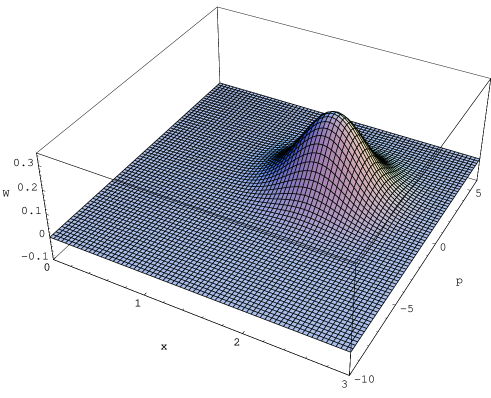
FIG. 8.: The Wigner function of the harmonic oscillator squeezed state, i.e. the multiphoton squeezed state (51) with $\gamma=0$, at $\beta_{1}=3$, $r=0.8$. The axes have been relabelled according to the “particle” language of phase space: $X_{1}\equiv x$, $X_{2}\equiv p$.

The planar section of the same Wigner function is also useful for later comparison, and it is shown in Fig. 9 below. We notice that it is centered at $X_{2}\equiv p=0$, and it is zero outside a small interval $[-5,5]$ of variation of $p$.

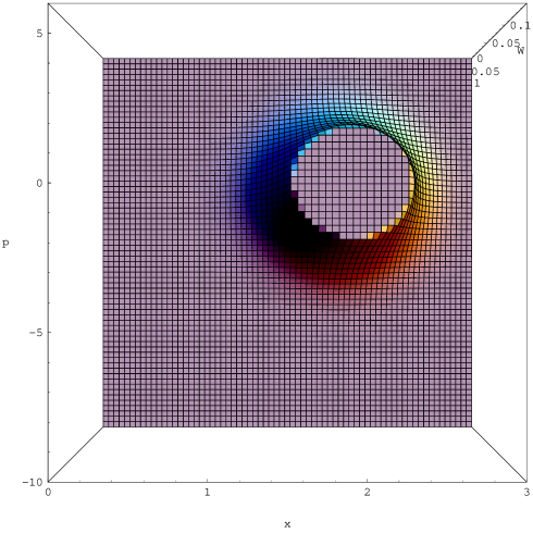
FIG. 9.: The planar section of the Wigner function for the harmonic oscillator squeezed state, i.e. the multiphoton squeezed state (51) with $\gamma=0$, at $\beta_{1}=3$, $r=0.8$.

Positivity of the Wigner function is preserved only by the multiphoton squeezed states with quadratic nonlinearity $F(X_{1})=X_{1}^{2}$. Even in this instance however, the Wigner function of the state (51) is displaced, rotated and deformed compared to the corresponding distribution with $\gamma=0$, as shown in Fig. 10 below.

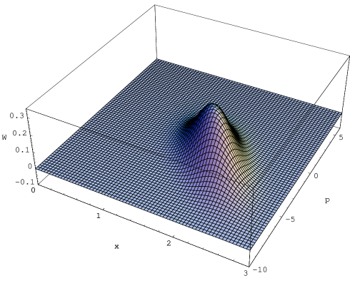
FIG. 10.: The Wigner function of the multiphoton squeezed state (51) with quadratic nonlinearity $F(X_{1})=X_{1}^{2}$, at $\beta_{1}=3$, $r=0.8$, and $\gamma=0.1$. Notice that it is not centered in $p=0$, and it is elongated and rotated compared to the purely squeezed case.

More insight can be gained by looking at its planar section. As shown in Fig. 11 the Wigner function of the multiphoton squeezed state exhibits an egg–shaped section (an elongated and deformed ellipsis). Therefore the area of overlap with the circular section associated to the generic number state of the harmonic oscillator in phase space gives rise to a nontrivial interference which is drastically modified with respect to the purely squeezed case originally discussed by Schleich, Walls and Wheeler [13], [14]. This fact is responsible for the behavior of the oscillations in the photon number distribution of a multiphoton squeezed state (see Fig. 1).

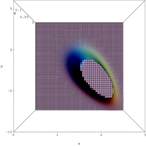
FIG. 11.: Planar section of the Wigner function for the multiphoton squeezed state (51) with $F(X_{1})=X_{1}^{2}$, $\beta_{1}=3$, $r=0.8$, and $\gamma=0.1$. The elliptic section of the Wigner function for the harmonic oscillator squeezed states is deformed into a egg–shaped section.

We see from Fig. 11 that besides the deformation of the elliptic shape, the Wigner function of the multiphoton squeezed state with quadratic nonlinearity, although still positive defined, it is translated and rotated compared to the purely squeezed case. In particular, it is not any more centered in $p=0$. Moreover it is elongated, and it is non zero only in the range of negative values $[0,-10]$ of $p$. The effects discussed above are significantly enhanced if we consider multiphoton squeezed states with higher nonlinearities. Starting with the next higher nonlinearity $F(X_{1})=X_{1}^{3}$ the Wigner function of the corresponding multiphoton squeezed state becomes very strongly deformed and acquires also negative values in some regions of the phase space. The Wigner function for the multiphoton squeezed state with cubic nonlinearity is reported in Fig. 12 below.

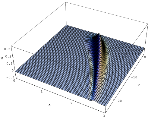
FIG. 12.: The Wigner function for the multiphoton squeezed state (51) with cubic nonlinearity $F(X_{1})=X_{1}^{3}$, and the same values of the parameters $\beta_{1}=3$, $r=0.8$, and $\gamma=0.1$ as in the quadratic case $F(X_{1})=X_{1}^{2}$. Notice that it becomes negative along a strip of values of $p$ ranging from $-2$ to $-24$ and of $x$ ranging from $1.4$ to $2.4$.

We notice that, compared to the case with quadratic nonlinearity, the Wigner function is more rotated, tending to place itself parallel to the $p$ axis. It is also much more elongated, as it is non zero for negative values of $p$ lying in the range $[0,-25]$. The planar section of the Wigner function for $F(X_{1})=X_{1}^{3}$ is plotted in Fig. 13 below.

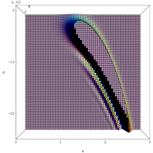
FIG. 13.: Planar section of the Wigner function for the multiphoton squeezed state (51) with cubic nonlinearity $F(X_{1})=X_{1}^{3}$, at values $\beta_{1}=3$, $r=0.8$, and $\gamma=0.1$.

We notice that the elliptic section becomes completely deformed into a narrowing “wing” for increasing negative values of $p$. Finally, in the case $F(X_{1})=X_{1}^{4}$ the Wigner function becomes even more twisted and shows many waves and ripples with negative and positive peaks, as shown in Fig. 14 below.

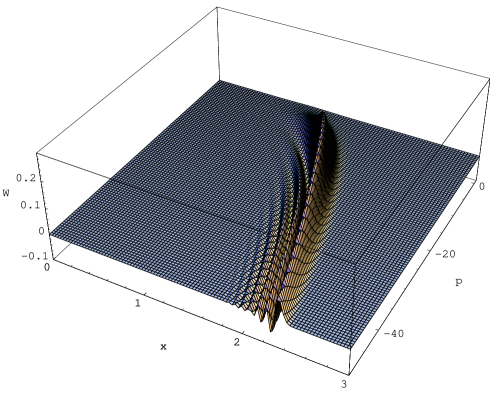
FIG. 14.: The Wigner function for the multiphoton squeezed state (51) with quartic nonlinearity $F(X_{1})=X_{1}^{4}$, at values $\beta_{1}=3$, $r=0.8$, and $\gamma=0.1$.

The planar section has the form reported in Fig. 15 below. It shows clearly the structure of the lateral waves and ripples of negative and positive peaeks. Besides, the central body is of still narrower “wing” section with further elongation, as the Wigner function is now non zero in the interval $[0,-50]$ of negative values of $p$.

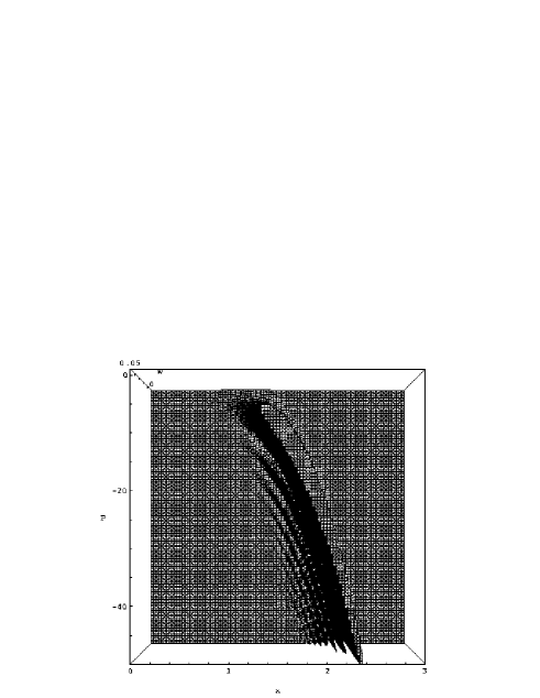
FIG. 15.: Planar section of the Wigner function for the multiphoton squeezed state (51) with quartic nonlinearity $F(X_{1})=X_{1}^{4}$, at values $\beta_{1}=3$, $r=0.8$, and $\gamma=0.1$.

VIII discussion and outlook

In the present work we have introduced a new class of nonclassical states of light. These new states have been obtained via a quadrature–dependent generalization of the linear Bogoliubov transformation first introduced by Yuen in his seminal work on the two–photon coherent states of light. We have shown that our quadrature–dependent Bogoliubov transformation, generated by a nonlinear operator function of the first quadrature is canonical under very broad constraints on the numerical coefficients of the transformation. The associated eigenstates of the transformation define a new class of nonclassical states that preserve some basic features of the coherent states of the harmonic oscillator such as classical nondispersive motion of the wave packet center. They also exhibit the amplitude squeezing typical of the squeezed states of the harmonic oscillator. However, the quadrature–dependent transformations generated by quadratic and/or higher powers of the first quadrature $X_{1}$ are associated to non quadratic effective Hamiltonians that summarize the interaction with media with higher nonlinearities (multiphoton down conversion processes) and we thus name them as multiphoton squeezed states. The presence of the quadrature–dependent term in the transformation is reflected in the presence of an additional phase factor in the wave function representation of these states. The interplay of the additional phase factor with the standard squeezing contributions is responsible for the remarkable nonclassical behavior exhibited by the field statistics, in particular by the photon number distribution and the second–order correlation function $g^{(2)}(0)$. The phase–space analysis in terms of the Wigner quasiprobability distribution shows that the multiphoton squeezed states are higly nonclassical, as the Wigner function is strongly deformed and it acquires negative values for cubic, quartic, and higher nonlinearities.

We have discussed the transformation generated by a nonlinear operator valued function of the first quadrature $X_{1}$. It is of course possible to introduce the transformations generated by a nonlinear operator valued function of the second quadrature $X_{2}$ and also by two nonlinear operator valued functions of each quadrature. However the treatment is in these cases slightly more tedious and involved, and will be deferred to a follow–up of the present work. In fact, looking at future developments, it will be interesting to explore the possibility, that we have only mentioned here, of considering quadrature–dependent transformations generated by operator valued functions more general than the simple powers considered in the present work. For instance, considering the transformation generated by a periodic function of the first quadrature might allowe to define squeezed states for massive particles interacting with optical lattices.

We should finally mention the possibility, in contexts broader than quantum optics, of exploiting the quadrature–dependent Bogoliubov transformation as a technical tool for the introduction of normal modes. In particular, we are currently investigating the possibility of applying the quadrature–dependent Bogoliubov transformation to the approximate diagonalization of the Hamiltonian of the weakly interacting Bose gas. The aim is to diagonalize a larger portion of the Hamiltonian in the many–body Hilbert space in comparison with the standard diagonalization originally performed via the linear Bogoliubov transformation [15].

REFERENCES

- [1] R. A. Fischer, M. N. Nieto, and V. D. Sandberg, Phys. Rev. D 29, 1107 (1984).
- [2] K. Wodkiewicz and J. H. Eberly, J. Opt. Soc. Am. B 2, 458 (1985).
- [3] J. A. Bergou, M. Hillery, and D. Yu, Phys. Rev. A 43, 515 (1991).
- [4] M. M. Nieto and D. R. Truax, Phys. Rev. Lett. 71, 2843 (1993).
- [5] M. M. Nieto and D. R. Truax, Phys. Lett. A 208, 8 (1993).
- [6] G. S. Prakash and G. S. Agarwal, Phys. Rev. A 50, 4258 (1994).
- [7] P. Marian, Phys. Rev. A 55, 3051 (1997); Phys. Rev. A 59, 3141 (1999).
- [8] G. S. Agarwal and K. Tara, Phys. Rev. A 43, 492 (1991).
- [9] V. V. Dodonov et al., Phys. Rev. A 58, 4087 (1998).
- [10] R. L. de Matos Filho and W. Vogel, Phys. Rev. A 54, 4560 (1996).
- [11] H. P. Yuen, Phys. Rev. A 13, 2226 (1976).
- [12] S. Wallentowitz, W. Vogel, and P. L. Knight, Phys. Rev. A 59, 531 (1999).
- [13] W. Schleich and J. A. Wheeler, Nature 326, 574 (1987).
- [14] W. Schleich, D. F. Walls, and J. A. Wheeler, Phys. Rev. A 38, 1177 (1988).
- [15] P. Nozieres and D. Pines, The Theory of Quantum Liquids Vol. II (Addison–Wesley, Reading, MA, 1990).