Quantum portfolios

Abstract

Quantum computation holds promise for the solution of many intractable problems. However, since many quantum algorithms are stochastic in nature they can only find the solution of hard problems probabilistically. Thus the efficiency of the algorithms has to be characterized both by the expected time to completion and the associated variance. In order to minimize both the running time and its uncertainty, we show that portfolios of quantum algorithms analogous to those of finance can outperform single algorithms when applied to the NP-complete problems such as 3-SAT.

Quantum computers can, if built, efficiently solve certain problems requiring exponential-time on a “classical” computer. Quantum algorithms currently come in two main varieties: the ones that rely on a Fourier transform [1], and the ones that rely on amplitude amplification [2]. Typically the algorithms consist of a sequence of trials. After each trial a measurement of the system produces a desired state with some probability determined by the amplitudes of the superposition created by the trial. Trials continue until the measurement gives a solution, so that the number of trials and hence the running time are random variables.

Strategies designed to optimize the performance algorithms with variable running time (called “Las Vegas” algorithms [3]), have recently gathered a lot of interest. First, restart strategies can improve the average performance of classical algorithms [4, 5, 6]. Second, portfolios analogous to those of finance can solve hard problems more effectively than any single technique [7]. Therefore an interesting question is how well these techniques developed for classical Las Vegas algorithms can apply to quantum computing.

Restart strategies have been examined in the context of Grover’s quantum search algorithm [2]. This algorithm consists of a number of trials repeated until a solution is found. Each trial has a predetermined number of iterations, which determines the probability of finding a solution. It is therefore necessary to carefully choose their number to optimize the running time.

Brassard et al. [8] showed how to optimize the expected running time of this algorithm by trading off a lower success probability after each measurement against fewer iterations in each trial. This amounts to a restart strategy. Unexpectedly, the result is an algorithm that is faster on average. Based on this result, [7] suggested that there may be a more desirable trade off between the expected search time and its variance, as in the return vs. risk trade off in finance. Here we perform this analysis in detail.

While the quantum restarts involved in this method are similar to restart strategies for classical Las Vegas algorithms, there are two distinctions. First, the number of iterations $t$ one performs before having a chance of finding a solution is chosen ahead of time. This isn’t so in the classical case, where the algorithm terminates as soon as a solution is found. Second, while the probability of finding a solution increases with time in the classical case, due to a monotonic cumulative probability distribution $F(t)$ of finding a solution after $t$ iterations, this isn’t so in the quantum case. For a quantum algorithm, the amplitudes after a trial with $t$ iterations determine the probability of finding a solution upon a measurement. This probability is non-monotonic and periodic [2].

Suppose there are $N$ possible states overall, and $S$ solutions to the search problem. After $t$ iterations of amplitude amplification the probability of finding a solution when measuring the state is

$$p_{t} = \sin^{2}((2t+1)\theta)$$ (1)

where $\theta$ satisfies $\sin^{2}\theta=S/N$. As pointed out in [9], if the number of solutions and hence $\theta$ is known, it is possible to determine the number of iterations $t^{*}$ necessary before a measurement is done such that the result is a solution state with near absolute certainty. Simply put, we need $(2t^{*}+1)\theta=\frac{\pi}{2}$ so that

$$t^{*}\approx\frac{\pi}{4}\sqrt{\frac{N}{S}}\approx 0.785\sqrt{\frac{N}{S}}$$ (2)

iterations are required in the limit of a small number of solutions.

Since the probability of finding a solution is already high for somewhat lower values of $t$, a lower expected running time can be obtained by a restart strategy, i.e. repeatedly running the quantum algorithm with a smaller number of iterations [9]. In particular, with $t$ iterations between every measurement, let $\eta_{t}$ be the number of iterations required to find a solution, which in itself is a random variable due to the variability in the number of trials. The expected number of iterations to find the solution is

$${\left\langle\eta_{t}\right\rangle}=\frac{t}{p_{t}}=\frac{t}{\sin^{2}((2t+1)\theta)}$$ (3)

In the limit of small $\theta\approx\sqrt{S/N}$, the optimal expected waiting time is [9]

$${\left\langle\eta^{*}\right\rangle} = \frac{z}{4\theta\sin^{2}(z/2)}\approx 0.690\sqrt{N/S}.$$ (4)

Boyer et al. [9] conclude that the restart strategy is indeed better, since the expected number of iterations $\eta^{*}$ is about $12\%$ smaller. However, this result is misleading if variance is considered as well. Specifically, a smaller number of Grover iterations between measurements no longer seems as attractive, since an improvement in the expected performance is traded off against an increase in the variance in the running time.

Put another way, one obtains a small gain in the expected waiting time by increasing the probability that we will need at least twice as many iterations. Quantitatively,

$${\left\langle\eta_{t}^{2}\right\rangle} = \sum_{k=1}^{\infty}(kt)^{2}p_{t}(1-p_{t})^{k-1}$$ (5)

$$= \frac{2-3p_{t}+p_{t}^{2}}{(1-p_{t})p_{t}^{2}}t^{2}$$ (6)

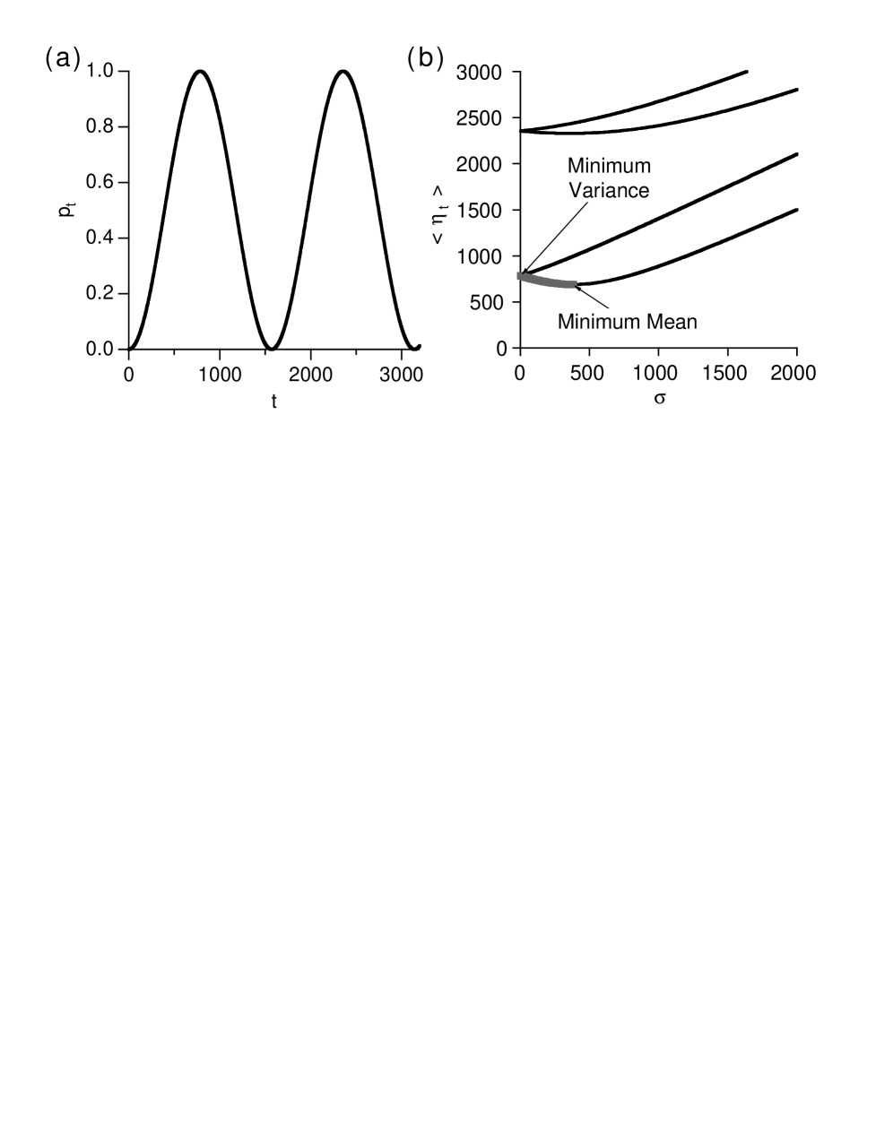
FIG. 1.: (a) Probability of measuring a solution state as a function of the number of Grover iterations $t$. (b) Expected running time vs. standard deviation for a quantum search algorithm, parameterized by the number of iterations between measurements. The efficient frontier is emphasized. In this figure $S/N=10^{-6}$.

Since ${\left\langle\eta_{t}\right\rangle}=t/p_{t}$, the standard deviation in the number of iterations, $\sigma$, is given by $\frac{t}{p_{t}}\sqrt{1-p_{t}}$. Figure 1 shows the “return vs. risk” curve in this case. The efficient frontier contains all the points for which the mean cannot be reduced without increasing the variance, and the variance cannot be reduced without increasing the mean. Any point on the efficient frontier is an acceptable strategy, and the choice of a strategy depends on a person’s preferences. The optimum choice will depend on the application. For example, in real-time applications, reducing variance will be more important than reducing the expected waiting time. On the other hand, in other domains, we may only care about the mean performance because we average over a large number of tries. Another possibility, common in finance, is to maximize the ratio of return to risk, ${\left\langle\eta_{t}\right\rangle}/\sigma$, called the Sharpe Ratio [10]. For the quantum search algorithm presented here, the restart strategy has a Sharpe Ratio near unity, while the strategy without restarts has a Sharpe ratio near infinity, because $p_{t}$ is close to one.

This discussion also applies to any quantum algorithm whose performance varies with the run time. This is the case of the Grover algorithm when the number of solutions is not known a priori [9] and quantum adiabatic algorithms of the type recently introduced by Farhi et al. [11].

Until now we considered variation in the number of iterations in each trial. Another approach applies to quantum algorithms with fixed trial lengths but with a variety of parameters that must be set prior to starting each trial. For a given problem instance, the choice of these parameters determines the probability for success of each trial. For example, instead of just adjusting phases based on whether states are solutions, such algorithms can use other efficiently-computable properties, as often used in conventional heuristic methods. In general, the best parameter choices for a given instance are not known a priori. Thus an important issue for such “quantum heuristics” is how to find choices that work well for typical problem instances encountered in practice.

As a specific example, we consider the $k$-satisfiability ($k$-SAT) problem. It consists of $n$ Boolean variables and $m$ clauses. A clause is a logical OR of $k$ variables, each of which may be negated. A solution is an assignment, i.e., a value, true or false, for each variable, satisfying all the clauses. An assignment is said to conflict with any clause it doesn’t satisfy. An example 2-SAT problem instance with 3 variables and 2 clauses is $v_{1}$ OR (NOT $v_{2}$) and $v_{2}$ OR $v_{3}$, which has 4 solutions, e.g., $v_{1}={\rm false}$, $v_{2}={\rm false}$ and $v_{3}={\rm true}$. For $k\geq 3$, $k$-SAT is NP-complete [12]. To consider typical rather than worst-case behavior, we focus on random 3-SAT, in which each clause is selected randomly, and take $m=4.25n$, which gives a high concentration of hard instances.

For a quantum algorithm [13], we use a superposition of all $N=2^{n}$ assignments, adjust phases based on the number of conflicts in each state and mix amplitudes among states based on their Hamming distances. The algorithm’s performance depends on how well the phase adjustments match the structure of the particular instance, which is not known a priori. One approach finds phase choices that work well on average for random 3-SAT problems [13], and gives better performance than amplitude amplification, which ignores problem structure.

However, phase adjustments that work well on average do not work well for all instances. Hence we can improve the performance by using a variety of choices, thereby reducing the chance of encountering instances that perform particularly poorly for any single choice of algorithm parameters. Such a “portfolio” of choices can reduce both the mean and variance of the time to find a solution.

In the simplest portfolio approach, we use different phase adjustments in each trial, instead of using the same ones every time. As we will show, this portfolio method is guaranteed to perform better than a fixed strategy, provided we have no other information concerning the performance of different choices.

To quantify this improvement, consider a variety of phase choices for a given instance. Each choice gives a particular success probability $p$ for a single trial. Let $f(p)$ be the distribution of success probabilities when selecting phase choices from among a prespecified set of possibilities.

The default strategy simply picks a single choice for the phase adjustments to use for every trial. In this case, the expected running time is ${\left\langle\frac{1}{p}\right\rangle}$, while the variance is ${\left\langle\frac{1-p}{p^{2}}\right\rangle}+\left({\left\langle\frac{1}{p^{2}}\right\rangle}-{\left\langle\frac{1}{p}\right\rangle}^{2}\right)$

Now assume that we randomly chose a different set of phases every time. Then the probability of success for a trial is simply ${\left\langle p\right\rangle}$. It follows that the mean and standard deviation are given by $\frac{1}{{\left\langle p\right\rangle}}$ and $\frac{1}{{\left\langle p\right\rangle}}\sqrt{1-{\left\langle p\right\rangle}}$, respectively.

Instead of using different choices for each trial, we can also use a “quantum portfolio” of our quantum algorithms. That is, all choices are evaluated simultaneously in superposition by using additional qubits to specify the particular phase choice.

For simplicity, consider such a portfolio of only two algorithms, i.e., choices for phases. A single qubit ${\left|a\right\rangle}=\alpha{\left|+\right\rangle}+\beta{\left|-\right\rangle}$ will determine which of the two algorithms is to be used.

Suppose the first choice gives amplitudes $c_{i}$ for state $i$ and the second gives $d_{i}$, when run individually. Then the result for the quantum portfolio is

$$\alpha\sum_{i}c_{i}{\left|i,+\right\rangle}+\beta\sum_{i}d_{i}{\left|i,-\right\rangle}$$ (7)

The probability of measuring a solution state is

$$p = |\alpha|^{2}\sum_{i\in A}|c_{i}|^{2}+|\beta|^{2}\sum_{i\in A}|d_{i}|^{2}$$ (8)

This probability is just a weighted sum of the individual success probabilities of each algorithm on its own. This discussion generalizes to combinations of additional phase choices. As a result, quantum portfolios of quantum algorithms, and mixed quantum algorithms, in which we randomly use a different quantum algorithm after each iteration, are equivalent, since they both result in the same probability of success at every measurement.

The surprising result is that such portfolios will complete faster on average that a computation with a fixed set of parameters. This is because

$${\left\langle\frac{1}{p}\right\rangle}\geq\frac{1}{{\left\langle p\right\rangle}}$$ (9)

always holds, since $p$ is strictly positive. Equality only occurs for a trivial probability distribution with only one outcome. This can be easily shown using the Schwarz inequality [14]:

$${\left\langle AB\right\rangle}^{2}\leq{\left\langle A^{2}\right\rangle}{\left\langle B^{2}\right\rangle},$$ (10)

for which equality holds only if there is a linear combination $aA+bB$ that is equal to zero with unit probability.

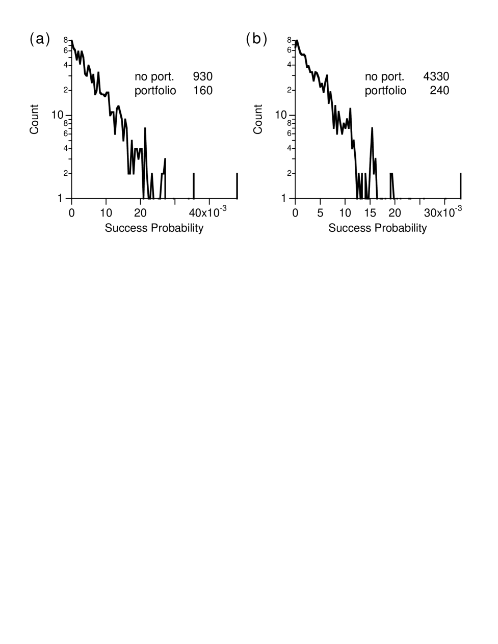
FIG. 2.: Distribution of success probabilities upon measurement of the quantum state for randomly chosen phases, for two different SAT instances with $n=8$. The numbers in the panel show the expected number of iterations with and without restarts.

The performance improvement obtained with such a strategy is shown in Figure 2, in which we randomly chose a different set of phases to use for each quantum computation between measurements. The histogram shows a substantial probability of choosing sets of phases with near zero probability of finding a solution after each measurement. This leads to a large expected waiting time if a portfolio isn’t used.

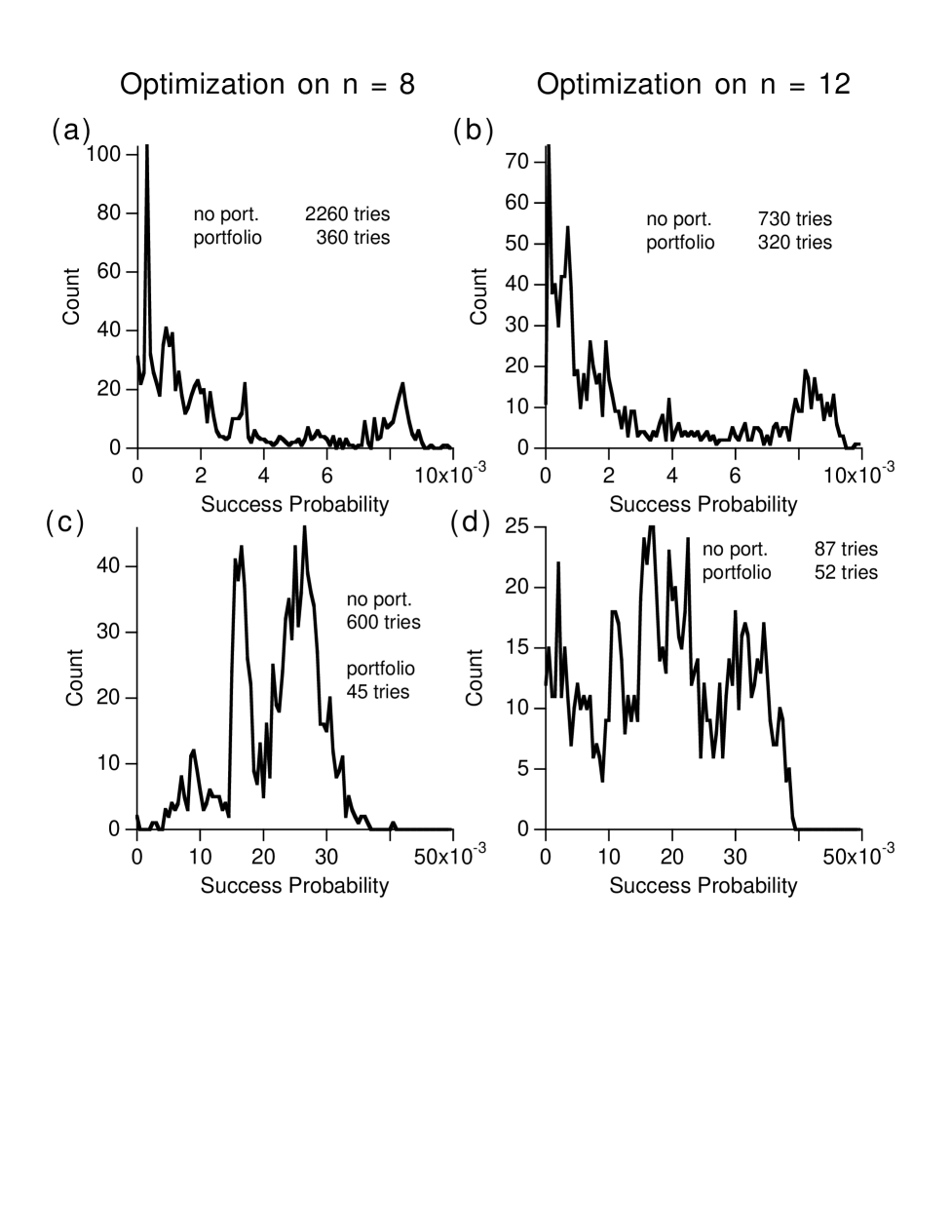
FIG. 3.: Distribution of success probabilities upon measurement of the quantum state for two 3-SAT problems with 20 variables. (a),(b) and (c),(d) correspond to two different problem instances. (a),(c) Random choice of phases optimized on instances with 8 variables. (b),(d) Random choice of phases optimized on instances with 12 variables. The expected number of measurements until a solution is found (based on the histograms) is indicated both for a single choice of parameters and a “portfolio” of parameters.

In practice, one would not use entirely random phases since their typical performance is rather low. Rather, one would use phases that are already known to work well for similar problems, e.g., obtained by optimizing the choices for a sample of similar problem instances. Optimizing choices for these sample instances multiple times, starting from a variety of initial choices, gives a set of phase choices that can be expected to perform much better than random choices on new instances drawn from the same problem ensemble as the training sample.

Since such optimization can be computationally demanding, a more feasible scenario performs this optimization on a large sample of small problems and then applies the resulting choices to new, larger instances. Thus algorithms are optimized on easily solvable instances, and applied to more difficult problems that have not been solved before.

For random $k$-SAT, the ratio of clauses to variables, $m/n$, characterizes the concentration of difficult instances so a reasonable scaling approach optimizes phases for small problems and then applies those to larger problems with the same ratio. Figure 3 shows the performance improvement of such a strategy. Here the set of phase choices available to select was created by optimizing for instances of 3-SAT with 8 and 12 variables and clause to variable ratio, $m/n$, of 4.25. These optimized phases were used to solve larger instances, with 20 variables. In this case, the advantages of a portfolio strategy are less dramatic than in Figure 2, but still quite impressive.

As a further observation, phases optimized for $n=12$ perform better on the $n=20$ instances than those optimized for $n=8$. Thus, the benefit of portfolios increases with the difference in size between those used to select phase choices and the instances of interest.

In the preceding, we considered a simple form of quantum portfolios, in which all available phase choices are evaluated simultaneously and independently for each trial. As with other quantum algorithms operating between measurements, such trials can be described by a single operator on the state in Equation 7. Since this operator does not itself involve a measurement, it can be used with amplitude amplification [9]. Thus while classical and quantum portfolios of quantum algorithms are equivalent when run as a series of trials, each ending with a measurement, the quantum portfolio allows a simple further improvement by combining it with amplitude amplification. That is, the expected performance improves from $1/{\left\langle p\right\rangle}$ to $O(1/\sqrt{{\left\langle p\right\rangle}})$.

Thus the advantages of classical portfolios can be improved on even further by a truly quantum portfolio. More generally, as with combining different conventional heuristics, we could consider operators within each trial that mix amplitude among the different quantum algorithms. Such operations provide a broader range of possible techniques than available with classical portfolios, though it remains to be seen whether such extensions give significant additional improvements.

REFERENCES

- [1] O. W. Shor, in Proceedings of the 35th Annual Symposium on the Foundations of Computer Science, edited by S. Goldwasser (IEEE Computer Society Press, Los Alamitos, CA, 1994), p. 124.
- [2] L. K. Grover, in Proceedings of the Twenty-Eighth Annual ACM Symposium on Theory of Computing (ACM, Philadelphia, PA, 1996), pp. 212–219.
- [3] R. Motwani and P. Raghavan, Randomized Algorithms (Cambridge University Press, New York, 1995).
- [4] H. Alt et al., Algorithmica 16, 543 (1996).
- [5] M. Luby, A. Sinclair, and D. Zuckerman, Information Processing Letters 47, 173 (1993).
- [6] C. P. Gomes and B. Selman, in Proceedings of the 13th Conference on Uncertainty in AI (UAI-97), edited by D. Geiger and P. Shenoy (Morgan Kaufmann, San Francisco, 1997), pp. 190–197.
- [7] B. A. Huberman, R. M. Lukose, and T. Hogg, Science 275, 51 (1997).
- [8] G. Brassard, P. Høyer, and A. Tapp, in Proceedings of 25th ICALP, Vol. 1443 of Lecture Notes in Computer Science (Springer, Heidelberg, 1998), pp. 820–831.
- [9] M. Boyer, G. Brassard, P. Høyer, and A. Tapp, Fortsch. Phys. 46, 493 (1998).
- [10] W. F. Sharpe, G. J. Alexander, and J. V. Bailey, Investments, 6th ed. (Prentice Hall, Upper Saddle River, NJ, 1999).
- [11] E. Farhi et al., Science 292, 472 (2001).
- [12] M. R. Garey and D. S. Johnson, Computers and Intractability: A Guide to the Theory of NP-Completeness (W. H. Freeman, San Francisco, 1979).
- [13] T. Hogg, Physical Review A 61, 052311/1 (2000).
- [14] W. Feller, An Introduction to Probability Theory and its Applications, 2 ed. (John Wiley & Sons, New York, 1971), Vol. 2.