Theory for the photon statistics of random lasers

Abstract

A theory for the photon statistics of a random laser is presented. Noise is described by Langevin terms, where fluctuations of both the electromagnetic field and of the medium are included. The theory is valid for all lasers with small outcoupling when the laser cavity is large compared to the wavelength of the radiation. The theory is applied to a chaotic laser cavity with a small opening. It is known that a large number of modes can be above threshold simultaneously in such a cavity. It is shown the amount of fluctuations is increased above the Poissonian value by an amount that depends on the number of modes above threshold.

I Introduction

A random laser is a laser where the necessary feedback is not due to mirrors at the ends of the laser but due to random scattering inside the medium wiersma:95a ; wiersma:97a ; beenakker:98b . It was long argued how to distinguish such a random laser from a random medium with amplified spontaneous emission (ASE) — in the former, the randomness is essential for providing feedback, whereas in the latter, scattering only increases the dwell-time in the medium and thus the amplification factor. Two years ago, the first experimental proof of a random laser was given cao:99a . It was demonstrated that the lasing action was indeed due to the randomness of the medium, by measuring the emitted radiation at different points on the surface of the sample and showing that the peaks in the radiation spectrum were completely different at different points.

Earlier experiments sha:94a ; lawandy:94a ; zhang:95a were only able to prove ASE in random media, frequently referred to as “laser-like emission”. In a medium with saturation both laser action and ASE lead to a dramatic narrowing of the emitted light profile upon crossing some threshold so that this criterion does not necessarily signal a laser. Most “traditional lasers” are characterized by emitting coherent radiation above threshold so that considering only the intensities and forgetting about the fluctuation properties is insufficient. Recently the first two measurements on the photon statistics of a random laser have been published. The group of Papazoglou reports that the emitted radiation becomes only partially coherent zacharakis:00a whereas the group of Cao reports that the statistics become completely Poissonian cao:01a .

The theoretical description of random lasers has in the past focused on the light intensity inside in the laser. Photons were considered as classical particles that diffuse or move in some other way repeatedly through the sample while being amplified. (The literature on this and similar methods is numerous, some more general, some more focusing towards a particular system; see e. g. Ref. wiersma:96a, for one of the earlier papers.) In this way the intensity of the emitted radiation can be computed, confirming the observed narrowing of the emission line far above threshold. No results for the fluctuation properties, however, can be derived in this way. Recently, random lasers are also simulated by the finite-difference time domain method (FDTD) taflove:95 . While this method in principle can incorporate quantum fluctuations on a microscopic level, the computational effort is prohibitively large, so that at most two-dimensional samples can be treated (see e. g. Ref. cao:00a, ), and most of its value is for one-dimensional applications (see e. g. Ref. jiang:00a, ). Furthermore, only short time series can be computed with acceptable effort so that the fluctuation properties of the emitted radiation are not accessible. A different, analytical, approach to noise in random lasers has recently been put forward by Hackenbroich et al. hackenbroich:01a . Since they do not include mode competition, their work is only applicable near threshold.

For a linear medium, i. e. a medium where, in contrast to a laser, saturation effects can be neglected, the statistics of the emitted radiation can be computed directly, e. g. by the method of input-output relations beenakker:98a . No theory of comparable power exists for lasers. The theoretical treatment of “non-trivial” lasers has in the past focused on the Petermann factor (see Refs. petermann:79a, ; siegman:89a, ; siegman:89b, for a definition). It is a geometry-related factor that describes by how much the excess noise of the emitted radiation is larger than for a “simple” single-mode laser — assuming that the non-trivial laser behaves the same way as a single-mode laser, which is basically equivalent to neglecting mode competition effects. (It should be stressed that the Petermann factor only gives information about the radiation far above threshold; it gives no information on threshold behavior.) Since the Petermann factor is a geometrical factor it can be computed for a linear medium and then used for the corresponding system filled with a medium with saturation. The Petermann factor has been derived for arbitrary geometries (see e. g. Ref. bardroff:99a, ; bardroff:00a, ) but also random media could be treated patra:00a ; frahm:00a ; schomerus:00a .

There thus is a need for a theory that allows one to compute the photon statistics of the emitted light for “non-trivial” lasers, in particular this includes random lasers. In this paper such a theory based on Langevin terms, also referred to as Langevin noise sources, is presented. Langevin terms have successfully been used to describe the radiation properties of linear media from a microscopic model bardroff:00a . On a higher level, they were used to describe random linear amplifying media mishchenko:99a where the Langevin terms included both fluctuations of the electromagnetic field and sample-to-sample fluctuations of the properties of the random medium. None of these theories included saturation effects of the medium so that they break down when the lasing threshold is approached. Apart from saturation effects for a single mode, a large number of modes can be above threshold simultaneously misirpashaev:98a , so that mode-competition is important and cannot be neglected.

This paper is organized as follows: In Sec. II the model for the photon statistics inside the laser is described and the model equations are derived. These are then solved in Secs. III and IV. Sec. V adds the necessary modifications to go from the fluctuations inside the laser to the fluctuations of the photocurrent emitted by the laser. Until this point all results are valid for arbitrary lasers, provided that the outcoupling is weak and the volume of the lasing medium is much larger than the cube of the wavelength. In Sec. VI we show how to apply the formalism developed in this paper to three exemplary systems and demonstrate thereby that it can indeed describe all relevant properties of lasing action. In Sec. VII the random laser is treated, and its photon statistics are computed. In Sec. VIII we try to explain the experimental results mentioned above. We conclude in Sec. IX.

II Model

We consider a optical cavity that is coupled to the outside by an opening that is small compared to the wavelength of the emitted radiation (see Fig. 1). Since the opening is small, there exist well-defined modes in the cavity, each with a well-defined eigenfrequency $\omega_{i}$, $i=1,\ldots,N_{\mathrm{p}}$, and a eigenmode profile $\Theta_{i}(\vec{r})$, and all modes are non-overlapping . (In the language of random lasers, this is a “resonant-feedback laser”.) Each mode $i$ thus can be described by the number $n_{i}$ of photons in it. Photons in mode $i$ can escape through the opening with rate $g_{i}$.

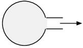
Figure 1: A (chaotic) cavity is coupled to the outside via a small opening. The cavity is filled with an amplifying medium. The light emitted through the opening is detected.

The cavity is filled with an amplifying medium. The medium is modeled by a four-level laser dye (see Fig. 2), where the lasing transition is from the third to the second level. The transition from the second level to the ground level is assumed to be so fast that the second level is always empty. The density of excited atoms (i. e. atoms in the third level) at point $\vec{r}$ in the cavity is $N(\vec{r})$. Excitations are created by pumping with rate $P(\vec{r})$ and can be lost non-radiatively with rate $a(\vec{r})$.

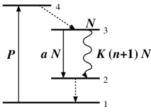
Figure 2: Amplification is modeled by a four-level system, where lasing action (marked by the wiggled line) is from the third to the second level. Dashed lines mark transitions that are much faster than the other ones and thus need not be included in the description.

Coupling between the electromagnetic field and the medium depends on two quantities, namely the eigenmode profile $\Theta_{i}(\vec{r})$ of mode $i$, and the transition matrix element $w(\omega)$ of the atomic transition $3\to 2$. [Frequently $w(\omega)$ will be a Lorentzian centered around some frequency $\Omega$.] The coupling of mode $i$ to the medium at point $\vec{r}$ is then given by $K_{i}(\vec{r})\equiv w(\omega_{i})|\Theta_{i}(\vec{r})|^{2}$.

The semiclassical equations of motion for $n_{i}$ and $N(\vec{r})$ are (the time argument for all quantities has been suppressed)

$$\dot{n}_{i} =-g_{i}n_{i}+\int d^{3}r\,(n_{i}+1)K_{i}(\vec{r})N(\vec{r})\;,$$ (1a)

$$\dot{N}(\vec{r}) =P(\vec{r})-a(\vec{r})N(\vec{r})-\sum_{i=1}^{N_{\textrm{p}}}(n_{i}+1)K_{i}(\vec{r})N(\vec{r})\;.$$ (1b)

“Semiclassical” means that all emission events, pumping events, …are assumed to be deterministic, with spontaneous emission described by the addition of a virtual photon to $n_{i}$ when computing the transition rates .

To include the randomness of all processes, Langevin terms have to be added to Eq. (1). The four random processes are the escape of photons (described by the Langevin term $\Gamma_{i}$), pumping [described by $\Phi(\vec{r})$], relaxation of the medium [described by $\alpha(\vec{r})$], and emission of a photon into mode $i$ at point $\vec{r}$ [described by $\Psi_{i}(\vec{r})$]. Each of these terms has zero mean, and a correlator that follows from the assumption that the elementary stochastic processes have independent Poisson distributions, hence

$$\langle\Gamma_{i}(t)\Gamma_{j}(t^{\prime})\rangle =\delta_{ij}\delta(t-t^{\prime})g_{i}\langle n_{i}\rangle\;,$$ (2a)

$$\langle\alpha(\vec{r},t)\alpha(\vec{r}\,^{\prime},t^{\prime})\rangle =\delta^{3}(\vec{r}-\vec{r}\,^{\prime})\delta(t-t^{\prime})a(\vec{r})\langle N(\vec{r})\rangle\;,$$ (2b)

$$\langle\Phi(\vec{r},t)\Phi(\vec{r}\,^{\prime},t^{\prime})\rangle =\delta^{3}(\vec{r}-\vec{r}\,^{\prime})\delta(t-t^{\prime})\langle P(\vec{r})\rangle\;,$$ (2c)

$$\langle\Psi_{i}(\vec{r},t)\Psi_{j}(\vec{r}\,^{\prime},t^{\prime})\rangle =\delta_{ij}\delta^{3}(\vec{r}-\vec{r}\,^{\prime})\delta(t-t^{\prime})\times$$

$$\hskip 39.83368ptK_{i}(\vec{r})\langle(n_{i}+1)N(\vec{r})\rangle\;.$$ (2d)

Eq. (2d) corresponds with the correlator given in Eq. (5b) of Ref. mishchenko:99a, .

Adding the terms from Eq. (2) to Eq. (1) gives the complete equations of motion:

$$\dot{n}_{i} =-g_{i}n_{i}+\Gamma_{i}+\int d^{3}\vec{r}(n_{i}+1)K_{i}(\vec{r})N(\vec{r})$$

$$\hskip 128.0374pt+\int d^{3}\vec{r}\,\Psi_{i}(\vec{r})$$ (3a)

$$\dot{N}(\vec{r}) =P(\vec{r})+\Phi(\vec{r})-a(\vec{r})N(\vec{r})+\alpha(\vec{r})$$

$$\hskip 28.45274pt-\sum_{i=1}^{N_{\textrm{p}}}(n_{i}+1)K_{i}(\vec{r})N(\vec{r})-\sum_{i=1}^{N_{\textrm{p}}}\Psi_{i}(\vec{r})$$ (3b)

The sign of the Langevin terms may be chosen freely as long as the term $\Psi_{i}(\vec{r})$ has the opposite sign in the equations for $\dot{n}$ and $\dot{N}$.

III Linearization

Eq. (3) cannot be solved by direct numerical methods since Langevin terms cannot be represented as “real” numbers. The only practicable way to proceed is to linearize the equations. First, we write $n_{i}=\bar{n}_{i}+\delta n_{i}$ and $N(\vec{r})=\overline{N}(\vec{r})+\delta N(\vec{r})$, where $\bar{n}_{i}\equiv\langle n_{i}\rangle$ and $\overline{N}(\vec{r})=\langle N(\vec{r})\rangle$ are the average solutions. We assume that these average solutions are identical to the solutions of the deterministic rate equation (1). This is equivalent to the factorizing approximation $\langle n_{i}N(\vec{r})\rangle\approx\langle n_{i}\rangle\langle N(\vec{r})\rangle$. For a single-mode cavity like used in cavity-QED this is a bad approximation, leading to errors of up to a factor $1/4$ in the computed average photon density, but if the number of modes in the cavity is large — which is the case that we are interested in — this factorization is valid rice:94a .

Inserting this solution, Eq. (3) can be reformulated so that only $\delta n_{i}$ and $\delta N(\vec{r})$ remain as variables. Linearization means that only terms proportional to $\delta n_{i}$ or $\delta N(\vec{r})$ are kept, i. e. terms proportional to $\delta n_{i}\delta N(\vec{r})$ are omitted. (This is justified as long as the variance is sufficiently smaller than the mean. This condition is equivalent to the validity of the factorizing approximation used above. It can be checked self-consistently from the computed results.) This way one arrives at an equation for the fluctuations alone, where the coefficients depend on the average solution:

$$\delta\dot{n}_{i} =-g_{i}\delta n_{i}+\Gamma_{i}+\int d^{3}\vec{r}(\bar{n}_{i}+1)K_{i}(\vec{r})\delta N(\vec{r})$$

$$\hskip 28.45274pt+\int d^{3}\vec{r}\delta n_{i}K_{i}(\vec{r})\overline{N}(\vec{r})+\int d^{3}\vec{r}\Psi_{i}(\vec{r})$$ (4a)

$$\delta\dot{N}(\vec{r}) =\Phi(\vec{r})-a(\vec{r})\delta N(\vec{r})+\alpha(\vec{r})-\sum_{i}(\bar{n}_{i}+1)K_{i}(\vec{r})\delta N(\vec{r})$$

$$\hskip 48.36958pt-\sum_{i}\delta n_{i}K_{i}(\vec{r})\overline{N}(\vec{r})-\sum_{i=1}^{N_{\mathrm{p}}}\Psi_{i}(\vec{r})$$ (4b)

For convenience, we will label the sum of the Langevin terms in Eq. (4a) as $f_{i}$, and the sum in Eq. (4b) as $g(\vec{r})$. Evaluating the Langevin terms from Eq. (2) at the average solutions $\bar{n}$ and $\overline{N}$ gives

$$\langle f_{i}f_{j}\rangle =\delta_{ij}\left[g_{i}\bar{n}_{i}+\int d^{3}\vec{r}(\bar{n}_{i}+1)K_{i}(\vec{r})N(\vec{r})\right]$$

$$=2\delta_{ij}g_{i}\bar{n}_{i}$$ (5a)

$$\langle g(\vec{r})g(\vec{r}\,^{\prime})\rangle =\delta^{3}(\vec{r}-\vec{r}\,^{\prime})\Bigl{[}a(\vec{r})P(\vec{r})+\overline{N}(\vec{r})$$

$$\hskip 85.35826pt+\sum_{i=1}^{N_{\mathrm{p}}}(\bar{n}_{i}+1)K_{i}(\vec{r})\overline{N}(\vec{r})\Bigr{]}$$

$$=2\delta^{3}(\vec{r}-\vec{r}\,^{\prime})P(\vec{r})$$

$$\langle f_{i}g(\vec{r})\rangle =-(\bar{n}_{i}+1)K_{i}(\vec{r})\overline{N}(\vec{r})$$ (5c)

IV Discretization and numerical solution

We now discretize the equations in space by picking points $\vec{r}_{j}$, $j=1,\ldots,N_{\mathrm{s}}$. Defining $K_{ij}\equiv K_{i}(\vec{r}_{j})$ and $N_{j}\equiv N(\vec{r}_{j})$ (analogously for all other quantities), the stationary densities $\bar{n}_{i}$ and $\overline{N}_{j}$ from Eq. (1) are the solution of the equations

$$g_{i}\bar{n}_{i} =\sum_{j=1}^{N_{\mathrm{s}}}(\bar{n}_{i}+1)K_{ij}\overline{N}_{j}\qquad(i=1,\ldots,N_{\mathrm{p}})$$ (6a)

$$P_{j} =a_{j}\overline{N}_{j}+\sum_{i=1}^{N_{\mathrm{s}}}(\bar{n}_{i}+1)K_{ij}\overline{N}_{j}\qquad(j=1,\ldots,N_{\mathrm{s}})$$ (6b)

This equation cannot be solved analytically but a numerical solution is straightforward (even though it may be numerically expensive if $N_{\mathrm{p}}$ and/or $N_{\mathrm{s}}$ are large).

Eq. (4) now becomes a linear ODE,

$$\frac{\mathrm{d}}{\mathrm{d}t}\left(\begin{matrix}\delta n_{i}\\ \delta N_{j}\end{matrix}\right)=\\ \left(\begin{array}[]{cc}-g_{i}+\sum_{j}K_{ij}\overline{N}_{j}&(\bar{n}_{i}+1)K_{ij}\\ -K_{ij}\overline{N}_{j}&-a_{j}-\sum_{i}(\bar{n}_{i}+1)K_{ij}\end{array}\right)\left(\begin{array}[]{c}\delta n_{i}\\ \delta N_{j}\end{array}\right)\\ +\left(\begin{array}[]{c}f_{i}\\ g_{j}\end{array}\right)$$ (7)

where it is understood that all indices $i$ run from $1$ to $N_{\mathrm{p}}$ and all indices $j$ from $1$ to $N_{\mathrm{s}}$, so that the previous equation can be written as a $(N_{\mathrm{p}}+N_{\mathrm{s}})$-dimensional matrix equation $\delta\mathcal{N}=\mathcal{A}\delta\mathcal{N}+\mathcal{L}$. Computing from $\mathcal{A}$ its matrix $\mathcal{U}$ of eigenvectors and its vector $\mathcal{E}$ of eigenvalues, the formal solution can immediately be written down as

$$\delta\mathcal{N}_{j}(t)=\sum_{k,l}^{1\ldots N_{\mathrm{p}}+N_{\mathrm{s}}}\int_{-\infty}^{t}\mathrm{d}t^{\prime}\,\mathcal{U}_{jk}\mathrm{e}^{\mathcal{E}_{k}(t-t^{\prime})}\mathcal{U}^{-1}_{kl}\mathcal{L}_{l}(t^{\prime})\;.$$ (8)

Since the vector $\mathcal{L}$ consists of Langevin terms, a numerically computed solution of Eq. (8) is not meaningful. Instead of $\delta\mathcal{N}_{j}(t)$ alone one has to consider correlators $\langle\delta\mathcal{N}_{j}(t)\delta\mathcal{N}_{j^{\prime}}(t)\rangle$. Noting that the $\mathcal{L}$’s are delta-correlated in time, and we are interested in $t\to\infty$ (as we are not interested in intermittent behavior when switching on the laser) we arrive at

$$\langle\delta\mathcal{N}_{j}\delta\mathcal{N}_{j^{\prime}}\rangle=-\sum_{klmn}^{1\ldots N_{\mathrm{p}}+N_{\mathrm{s}}}\frac{\mathcal{U}_{jm}\mathcal{U}_{j^{\prime}n}\mathcal{U}^{-1}_{mk}\mathcal{U}^{-1}_{nl}}{\mathcal{E}_{m}+\mathcal{E}_{n}}\langle\mathcal{L}_{k}\mathcal{L}_{l}\rangle\;.$$ (9)

Inserting the expectation values of the correlators from Eq. (5) gives the final result where a numerical solution is easy once the average solution $\bar{n}_{i}$, $\overline{N}_{j}$ is known. ($\langle\mathcal{L}_{k}\mathcal{L}_{l}\rangle$ has to evaluated at the average solution and does thus not depend on time.)

V Outcoupling

So far we have considered the number of photons $n_{i}$ in the $i$-th mode inside the cavity. For practical purposes one is more interested in the photo current $I$ emitted from the cavity. ($I$ gives the number of photons emitted per unit time and is thus equal to the photon flux integrated over the entire cross-sectional area.) Even though the photons from different modes $i$ are emitted through the same opening, each mode has a distinct frequency $\omega_{i}$ so that the modes are easily distinguished on the outside. We can thus define the photo current $j_{i}(t)\equiv\bar{j}_{i}+\delta j_{i}(t)$ through the opening due to the $i$-th mode in the cavity. The photo current can for example be measured by an (ideal) photodetector that absorbs the emitted photons. The fluctuations of the photo current within some time $\tau$ (we assume the limit $\tau\to\infty$) are quantified by the noise power

$$P_{i}=\lim_{\tau\to\infty}\frac{1}{\tau}\int_{-\tau/2}^{\tau/2}dt\,\delta j(0)\delta j(t)\;.$$ (10)

The ratio $\mathcal{F}_{i}=P_{i}/\bar{j}_{i}$ is called the Fano factor and is frequently used to describe the fluctuation properties of optical radiation.

In Sec. II we have introduced the loss rates $g_{i}$. From their definition it is obvious that the mean photo current $\bar{j}_{i}$ is

$$\bar{j}_{i}=g_{i}\bar{n}_{i}\;.$$ (11)

To also compute the fluctuations $\delta j_{i}$ we need to treat the outcoupling in more detail. In a traditional laser (see Fig. 3) the loss rate $g_{i}$ is given by the ratio of the transmission probability $t_{i}$ (in classical optics referred to as “transmittivity”) through the outcoupling mirror and the round-trip time $T$ through the cavity,

$$g_{i}=t_{i}/T\;.$$ (12)

The transmission through the outcoupling mirror changes the noise of the signal compared to the noise inside the cavity, and the Fano factor of the emitted radiation is patra:00b

$$\mathcal{F}_{i}=t_{i}\frac{\langle\delta n_{i}\delta n_{i}\rangle}{\bar{n}_{i}}+1-t_{i}\;.$$ (13)

This equation can, apart from following the quantum-optical approach of Ref. patra:00b, , also be understood by the following simple argument: The fraction $\langle\delta n_{i}\delta n_{i}\rangle/\bar{n}_{i}$ on the right-hand side is the Fano factor of the radiation trapped inside the cavity in mode $i$. With probability $t_{i}$ the detector will “see” the radiation inside the cavity, and with probability $1-t_{i}$ it will see reflected vacuum fluctuations (which have a Fano factor equal to $1$).

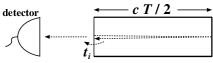
Figure 3: The loss rate of photons inside the cavity is given by the ratio of the probability $t_{i}$ that a photon incident on the outcoupling mirror is transmitted and the time $T$ needed for one round trip through the cavity. The photons emitted from the cavity are detected by an ideal photodetector.

The Fano factor for a measurement where the photons emitted from the cavity in all modes are detected simultaneously is

$$\mathcal{F}=\frac{\sum_{i}t_{i}^{2}\langle\delta n_{i}\delta n_{i}\rangle}{\sum_{i}t_{i}\bar{n}_{i}}+\frac{\sum_{i}t_{i}(1-t_{i})\bar{n}_{i}}{\sum_{i}t_{i}\bar{n}_{i}}\;.$$ (14)

It is immediately obvious that $t_{i}$ and $g_{i}$ can for a traditional laser be identified by properly choosing the unit of time (for the simple laser from Fig. 3: by choosing $T$ as the unit of time). We will show in Sec. VII that this is also possible for a random laser. In the following when giving numerical values or distribution functions for $g_{i}$ this identification has been made.

Figure 4: Comparison of the Fano factor $\mathcal{F}$ for three different conditions. The left axis (solid line) depicts the Fano factor for the integrated emitted radiation, the right axis (dashed line) for the lasing mode only. (a) Laser with just a single mode. (b) Laser with a cavity supporting $10$ modes where one mode is coupled out much less than the others, thus effectively modeling a single-mode laser with $\beta\approx 0.1$. (c) Laser with $10$ identical modes.

VI Comparison of lasing regimes

To demonstrate the application of the formalism presented in this paper and the validity of the approximations made in this paper we first want to discuss three simple cases not involving random media. For simplicity we set $a\equiv w\equiv 1$, $N_{\mathrm{s}}=N_{\mathrm{p}}$ and $K\equiv\mathrm{const}$. This reduces the number of parameters significantly without reducing the physical content.

The physical features of a laser (in contrast to a linear amplifier) are easily understood in the following picture: A certain number of excited atoms are created by pumping within a certain time, and each of those excitations has to be “consumed” either by nonradiative relaxation or by emitting one photon from the cavity. For high photon number in the cavity, nonradiative relaxation can be neglected, and each pumping event eventually leads to the emission of one photon from the cavity. The fluctuations of the integrated photo current are thus equal to the fluctuations of the pump source, assumed to be Poissonian throughout this paper.

In Fig. 4(a) the single-mode laser ($N_{\mathrm{p}}=1$) with a small opening ($g=10^{-2}$) is treated. The computed curve reproduces the features of a “traditional” laser. The precise location of the maximum is somewhat off (see the discussion of the factorization approximation above, or refer to Ref. herzog:00a for a more detailed discussion of the effects of different approximations on the computed curve near the lasing threshold) but its height reproduces the exact quantum-mechanical value well. For high values of the pumping, the photon statistics of the emitted radiation becomes Poissonian, as qualitatively explained above.

In Fig. 4(b) we have modeled a laser with one mode coupled to the outside with $g=10^{-2}$ and the other $9$ modes with $g=10^{-1}$, hence $N_{\mathrm{p}}=10$. (The value $g=10^{-2}$ was chosen for scaling the axes of the figure.) The mode with the smallest $g$ will be the lasing mode, whereas radiation in the other modes quickly escapes to the outside so that no significant number of photons can accumulate in those modes. This basically models a single-mode laser where only a fraction $\beta=1/N_{\mathrm{p}}$ of the spontaneous radiation is emitted into the lasing mode. ($\beta$ is called the spontaneous emission factor. An ideal cavity-QED laser has $\beta=1$ whereas a semiconductor laser can have a $\beta$ as low as $\beta=10^{-8}$.) The behavior is similar to Fig. 4(a), except that the peak of the Fano factor of the lasing mode is larger by about a factor $8$. For small beta, one expects a scaling $\propto\beta^{-1/2}\approx 3$ rice:94a but $\beta=1$ and $\beta=0.1$ are too large for that scaling to be exactly valid.

In Fig. 4(c) the system is kept at $N_{\mathrm{p}}=10$ with all $g_{i}\equiv 10^{-2}$. The total radiation depicts the same qualitative behavior as for the two cases presented so far but the radiation emitted by the lasing mode alone (in this case: by an arbitrary but fixed mode) depicts a completely different picture: The Fano factor diverges as the pumping is increased. This is easily understood by the qualitative description given above. For high pumping, every pump excitation eventually results in one photon being emitted from the cavity, but if there are several lasing modes the photon still has the freedom to chose one of those modes. These additional fluctuations can be that large that they eventually lead to a very large Fano factor for large pumping. (It is obvious that the Langevin approach will break down eventually if the fluctuations become too large, as explained above.)

The three test cases show that the model presented here is able to explain all relevant features of a laser.

VII Random laser

A random laser is a laser where the feedback is not due to mirrors at the ends of the laser but due to chaotic scattering, either caused by scatterers placed at random positions or by a chaotic shape of the cavity wiersma:95a ; beenakker:98b . If the mean outcoupling is weak a large number of modes in the cavity can be above threshold simultaneously misirpashaev:98a . As seen above, mode competition introduces additional noise into the modes. However, even if there are several modes above threshold, there only will be mode competition if the modes are spatially overlapping and thus are “eating” from the same excitations. The main purpose of this paper is to answer the question whether in a random laser there is a relevant level of mode-competition noise or whether the radiation emitted in a laser line approaches Poissonian statistics for strong pumping – both statements are mutually exclusively.

We consider a chaotic cavity as depicted in Fig. 1 with a small opening to the outside. This problem becomes a stochastic problem by considering an ensemble of cavities with small variations in shape or scatterer positions. The coefficients appearing in Eq. (6) thus become random quantities. The statistics of these coefficients for a chaotic cavity with small opening is known beenakker:97a ; guhr:98a . The mean loss rate $\bar{g}$ of a cavity with volume $V$ through a hole of diameter $d$ at frequency $\omega$ is bethe:44a

$$\bar{g}=\frac{16\pi^{2}d^{6}\omega^{6}}{c^{6}}\cdot\frac{\pi^{2}c^{3}}{\omega^{2}V^{2}}\equiv\bar{t}\cdot\delta\;.$$ (15)

$\delta$ is the level spacing of the cavity. Its inverse $1/\delta$ is the time needed to explore the entire phase space inside the cavity and can be identified with the round-trip time introduced for a “traditional laser” in Eq. (12).

In a chaotic cavity the modes $\Theta_{i}(\vec{r})$ can be modeled as random superpositions of plane waves berry:77a . This implies a Gaussian distribution for $\Theta_{i}(\vec{r})$ at any point $\vec{r}$ . The loss rate $g_{i}$ is proportional to the square of the gradient of $\Theta(\vec{r})$ normal to the opening at the opening, hence its distribution is

$$\mathcal{F}(g_{i})=\frac{\mathrm{e}^{-2g_{i}/\bar{g}}}{\sqrt{2\pi g_{i}\bar{g}}}\;,$$ (16)

and $g_{i}$ and $g_{j}$ are uncorrelated for $i\neq j$.

It should be noted that the level spacing $\delta$ is no random quantity, so that $g_{i}$ and $t_{i}$ can be identified by choosing $1/\delta$ as the unit of time.

For simplicity we assume that the amplification profile $w\equiv 1$ so that the distribution of the eigenfrequencies is not needed to compute $K_{ij}$. (The distribution is known beenakker:97a so that an extension to non-constant $w$ is straightforward.)

Figure 5: Fano factor of the radiation emitted from the (primary) lasing mode (left axis, solid line) of some particular sample. The right axis (dashed line) depicts the number of modes above lasing threshold. Each additional mode crossing the threshold increases the Fano factor of the primary lasing mode.

Fig. 5 shows the computed Fano factor for a particular sample from this ensemble ($N_{\mathrm{p}}=10$, $\bar{g}=0.5$ but remember that the value of $g$ of the lasing mode is much smaller than $\bar{g}$ patra:00a ; schomerus:00a ). This kind of curve is typical for all members of the ensemble, while the precise shape varies. When the first mode crosses the lasing threshold, the Fano factor goes through a maximum. While there is a global decrease with increasing pumping, additional peaks are superimposed each time another mode crosses the lasing threshold. (In the following a mode is considered to be above lasing threshold if it contains at least $2$ photons but the results are basically independent of whether one chooses $1$, $2$ or $10$ photons.) The Fano factor approaches $1$ plus some finite difference. Mode-competition noise thus gives a contribution to the noise but there still exists a lasing threshold that is well-defined by a peak of $\mathcal{F}$.

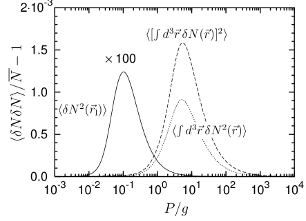
Figure 6: Fluctuations of the excitation density $N(\vec{r})$ of the medium for the sample from Fig. 5. Depicted are the fluctuations $\langle\delta N^{2}(\vec{r}_{\mathrm{l}})\rangle/\overline{N}(\vec{r_{\mathrm{l}}})$ at the point $\vec{r}_{\mathrm{l}}$ where the eigenmode profile of the primary lasing mode has the largest magnitude (solid line, scaled by a factor $100$), and the global quantities $\langle[\int d^{3}\vec{r}\,\delta N(\vec{r})]^{2}\rangle/\int d^{3}\vec{r}\overline{N}(\vec{r})$ (long dashes) and $\langle\int d^{3}\vec{r}\,\delta N^{2}(\vec{r})\rangle/\int d^{3}\vec{r}\overline{N}(\vec{r})$ (short dashes).

Similarly to computing the fluctuations of the Fano factor, it is possible to compute the fluctuations $\delta N(\vec{r})$ of the density of excited atoms directly from Eq. (9). Fig. 6 depicts the computed fluctuations for the entire cavity (dashed lines) as well as for the point $\vec{r}_{\mathrm{l}}$ where the eigenmode profile $\Theta_{l}(\vec{r})$ of the primary lasing mode has the largest magnitude. The former quantity peaks at a significantly larger pumping $P$ which is immediately understood by noticing that the primary lasing mode effects only part of the total cavity, and a significant part of the cavity is left “untouched” until more modes have crossed the lasing threshold.

Figure 7: The value of the Fano factor for the primary lasing mode depends on the number $N_{\mathrm{l}}$ of cavity modes above laser threshold, not on the other parameters. Unless otherwise noted, computed from $\approx 9\cdot 10^{5}$ samples with $\bar{g}=0.1$. (a) Probability distribution of $(\mathcal{F}-1)/g$ for $\bar{g}=0.1,0.2,\ldots,0.5$. The five curves overlap almost perfectly, thereby demonstrating that the size of the opening does not influence the amount of mode-competition noise generated. (Computed from $\approx 10^{5}$ samples for each value of $\bar{g}$ with identical realizations for $K_{ij}$ and $g_{i}/\bar{g}$ for the five runs.) The inset shows the probability distribution from the large set with $\bar{g}=0.1$ plotted logarithmically. (b) Average of the Fano factor as a function of the outcoupling constant $g$ of the lasing mode. (c) Average of the Fano factor as a function of $N_{\mathrm{l}}$.

The two global quantities depicted, $\langle[\int d^{3}\vec{r}\,\delta N(\vec{r})]^{2}\rangle/\int d^{3}\vec{r}\overline{N}(\vec{r})$ and $\langle\int d^{3}\vec{r}\,\delta N^{2}(\vec{r})\rangle/\int d^{3}\vec{r}\overline{N}(\vec{r})$, differ by the inclusion of terms $\langle N(\vec{r}_{1})N(\vec{r}_{2})\rangle$, $\vec{r}_{1}\neq\vec{r}_{2}$. The different heights of the peaks (the first one is higher) demonstrate that (at least in the relevant interval of $P$, and on average) the density of excited atoms at different positions is positively correlated. This can be understood in the following simple picture: The photon densities $n_{i}$ and the excitation densities $N(\vec{r})$ are on average negatively correlated since each emission of an extra photon ($\delta n_{i}>0$) leads to the de-excitation of an atom [$\delta N(\vec{r})<0$], and vice versa, hence $\langle n_{i}\delta N(\vec{r})\rangle<0$. [This has also been confirmed by computing this correlator numerically from Eq. (9)]. Since the excited atoms at different positions communicate only via the radiation field, their density thus has to be positively correlated.

It is difficult to relate the fluctuations of the excitation density of the medium to the properties of the emitted light. With increasing pumping, a peak of $\langle\delta N^{2}(\vec{r}_{\mathrm{l}})\rangle/\overline{N}(\vec{r_{\mathrm{l}}})$ starts to form (cf. Fig. 6) at the same pumping that a peak starts to form for the Fano factor $\mathcal{F}$ (cf. Fig. 5) but the location of the maximum of the peak is significantly different for both curves. The complicated interplay between radiation modes and matter in a random laser does not allow for a simple understanding of the relation between these two quantities, and we will not discuss the fluctuations of the medium further in this paper since it focuses on the radiation properties. The complicated structure of the eigenmodes of a chaotic cavity is what makes a random laser fundamentally different from a “traditional” laser.

In the following we will concentrate on the radiation and on the Fano factor far above threshold. $P$ is chosen such that $P/g\approx 10^{7}$ (remember that the value of $g$ of the lasing mode fluctuates). This is a compromise between a so large value as possible to ensure that the limiting value for $P\to\infty$ is approached as closely as possible, and a not too large value of $P$ to avoid numerical problems (remember that Fig. 5 already spans $11$ orders of magnitude).

The main results of a Monte-Carlo simulation with $N_{\mathrm{p}}=10$ are depicted in Fig. 7. The scaled Fano factor does not depend on the size of the opening (Fig. 7a), and only weakly on the outcoupling constant of the lasing mode (Fig. 7b). As Fig. 7c clearly shows, the true dependence is on the number $N_{\mathrm{l}}$ of modes above threshold. (The weak dependence of the Fano factor on the value of $g$ of the lasing mode can be understood by noting that $N_{\mathrm{l}}$ is correlated with $g$ of the lasing mode.) The finite value of $\mathcal{F}-1$ thus indeed is due to mode competition noise, as claimed above.

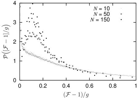
Figure 8: Distribution of the scaled Fano factor for cavities with different number $N_{\mathrm{p}}=N_{\mathrm{s}}$ of modes.

For larger cavities, i. e. cavities with more modes in it, the distribution of $(\mathcal{F}-1)/g$ changes from a peak near $\mathcal{F}=1$ to one that peaks at a finite value of $(\mathcal{F}-1)/g$, as seen from Fig. 8. As $N_{\mathrm{p}}$ and $N_{\mathrm{s}}$ increase, the effort to numerically compute the average solution from Eq. (6) increases very fast, so that only a comparably small number of realizations were computed ($\approx 20000$ for $N_{\mathrm{p}}=50$ and $\approx 4000$ for $N_{\mathrm{p}}=150$), explaining the large sampling error in the histograms. [The speed could be increased significantly by developing an optimized algorithm for solving Eq. (6).] For larger $N_{\mathrm{p}}$ the average of $(\mathcal{F}-1)/g$ becomes smaller as the large-$\mathcal{F}$ tail gradually disappears. (From $N_{\mathrm{p}}=10$ to $N_{\mathrm{p}}=150$ the average becomes smaller by about a factor 2; the average is difficult to compute since it sensitively depends on few samples with large $\mathcal{F}$.)

VIII Interpretation of experiments

Experiments on random lasers are usually explained by the formation of small “virtual” cavities, which can “trap” laser light, so that it is scattered within a small volume many times before it can escape; see Fig. 9. (The linear dimension of such cavities was measured to be of the order of $100$ wavelengths cao:99a ). The chaotic cavity used as model in this paper should be understood as representing one of those virtual cavities. It is not obvious which values of the parameters ($N_{\mathrm{p}}$, $N_{\mathrm{s}}$, $g_{i}$, …) are needed to explain the experiments. In the following we will argue that the important parameters are the average outcoupling $\bar{g}$ and, even more importantly, the probability distribution $\mathcal{P}(g_{i}/\bar{g})$ as they together determine the number $N_{\mathrm{l}}$ of modes above lasing threshold.

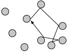
Figure 9: Small “virtual” cavities can be formed by scatterers in the random medium. Photons can be trapped very efficiently (i. e. small outcoupling) if the distances between the scatterers are compatible with the wavelength of the radiation).

Above it was shown that $N_{\mathrm{p}}$ and $N_{\mathrm{s}}$ influence the Fano factor only weakly, i. e. only by a factor $2$, and thus much smaller than the difference observed in the experiments. Even though it was not explicitly discussed in this paper, it is obvious that the choice of $w(\omega)$ and $\Theta_{i}(\vec{r})$ will not be important, either. This leaves $\bar{g}$ and $\mathcal{P}(g_{i}/\bar{g})$ as parameters to explain the experiments.

In this paper, a random laser is modeled by a chaotic cavity with a small opening. The size of the opening determines the average outcoupling $\bar{g}$, and all $g_{i}$ scale linear with $\bar{g}$ [see Eq. (16)]. For a virtual cavity the average outcoupling cannot be computed in such a simple geometrical way. The outcoupling $g_{i}$ for the $i$-th mode in such a virtual cavity depends delicately on the positions of the scatterers and the wavelength of that mode. While no theory is available to compute $g_{i}$ or at least $\bar{g}$ for this case, it is likely that it will be relatively large as individual scatterers cannot be as effective as a massive wall with only one small opening.

It was shown in Fig. 7a that $\mathcal{F}-1\propto\bar{g}$. This is valid as long as the size of the opening is small compared to the square of the wavelength. If the opening becomes larger, the modes inside the cavity acquire a finite width (in frequency space) and start to overlap, severely complicating the theory , and it is not obvious how the behavior changes. Cao cao:01a speculates that this overlapping prevents the formation of a fixed photon number in one particular mode as photons are constantly exchanged between modes with nearby frequencies. Furthermore, the Petermann factor of the lasing mode becomes significantly large frahm:00a which might or might not increase the amount of fluctuations. While there is no proof that the amount of fluctuations is increased by these two effects, it seems to be obvious that the amount of fluctuations will not decrease due to them. Hence, $\mathcal{F}-1$ will at least increase proportional to the size of the opening — also for openings that are larger than the region of validity of the theory presented in this paper.

The previous argument assumes that the number $N_{\mathrm{l}}$ of lasing modes inside a virtual cavity is the same as for a chaotic cavity with a small hole. Mode-overlap itself does not change that number but for a larger opening the distribution function $\mathcal{P}(g_{i}/\bar{g})$ no longer has the form given by Eq. (16). The form of $\mathcal{P}(g_{i}/\bar{g})$ sensitively depends on the kind of outcoupling, and the number of lasing modes in turn sensitively depends on $\mathcal{P}(g_{i}/\bar{g})$. For example, there already is a large difference between a cavity with one small hole and a cavity with two somewhat smaller holes (so that the total average loss rate is the same in both cases) misirpashaev:98a . It is very well possible that the form of $\mathcal{P}(g_{i}/\bar{g})$ may look significantly different from Eq. (16) and could depend on many parameters of the sample.

The differences in $\mathcal{P}(g_{i}/\bar{g})$ and thus in the number of lasing modes are thus the natural candidates to explain the differences observed in the two experiments.

This prediction could in principle be checked experimentally by measuring the number of modes above threshold in one virtual cavity but to devise an experimental setup to do this seems very difficult, if at all possible. The sample used by the group of Papazoglou zacharakis:00a should have several spatially overlapping modes above lasing threshold (i. e. some modes above threshold are in the same virtual cavity), whereas in the sample by Cao cao:01a all modes above lasing threshold should be spatially separated (i. e. be in different virtual cavities). One explanation could be that Cao’s sample has more resonant feedback, so that the confinement of the lasing modes is stronger, compared to Papazoglou’s sample. In the latter, the modes would be extended over a much larger part of the sample (i. e. the virtual cavities are larger), giving them more possibility to overlap.

IX Conclusions

In this paper we have developed a theory to compute the fluctuation properties of the radiation of a random laser. While for a standard single-mode laser the emitted radiation becomes coherent far above threshold, the radiation for a random laser is fluctuating more. It was shown that this extra noise is due to mode competition noise, i. e. due to the uncertainty of deciding into which mode to photon is emitted by induced emission. This noise is larger the higher the number of modes above lasing threshold is.

To be able to create mode competition noise, the competing modes have to be (at least partially) overlapping. On the other hand, if the profiles of the modes are overlapping too much, usually only one of those modes will be above threshold. The amount of noise created thus is the result of a delicate interplay between these two competing effects. For a random laser modeled by a chaotic cavity filled with a laser dye, this leads to a finite increase of the Fano factor far above threshold, with the precise value depending on the number of modes within the cavity that are simultaneously above threshold for that particular realization of the disorder. In particular, the emitted radiation becomes coherent if only one mode is above threshold.

Recent experiments on random lasers zacharakis:00a ; cao:01a gave conflicting results on whether the noise is increased with respect to the Poissonian value. Even though it is not directly possible to model the differences in the two experiments, the theory presented in this paper suggests that this is due to the differences in the the number of modes above threshold. This number depends heavily on the specific system in question, so that the noise properties of a random laser are not universal but depend on the (experimental) setup.

- (1) D. S. Wiersma, M. P. van Albada, and A. Lagendijk, Nature 373, 203 (1995).
- (2) D. S. Wiersma and A. Lagendijk, Physics World 10, 33 (1997).
- (3) C. W. J. Beenakker, in Diffuse Waves in Complex Media, edited by J.-P. Fouque (Kluwer, Dordrecht, 1999), vol. 531 of NATO Science Series C, pp. 137–164.
- (4) H. Cao, Y. G. Zhao, S. T. Ho, E. W. Seelig, Q. H. Wang, and R. P. H. Chang, Phys. Rev. Lett. 82, 2278 (1999).
- (5) W. L. Sha, C.-H. Liu, and R. R. Alfano, Opt. Lett. 19, 1922 (1994).
- (6) N. M. Lawandy, R. M. Balachandran, A. S. L. Gomes, and E. Sauvain, Nature 368, 436 (1994).
- (7) D. Z. Zhang, B. Y. Cheng, J. H. Yang, Y. L. Zhang, W. Hu, and Z. L. Li, Opt. Commun. 118, 462 (1995).
- (8) G. Zacharakis, N. A. Papadogiannis, G. Filippidis, and T. G. Papazoglou, Opt. Lett. 25, 923 (2000).
- (9) H. Cao, Y. Ling, J. Y. Xu, C. Q. Cao, and P. Kumar, Phys. Rev. Lett. pp. 4524–4527 (2001).
- (10) D. S. Wiersma and A. Lagendijk, Phys. Rev. E 54, 4256 (1996).
- (11) A. Taflove, Computational Electrodynamics: The Finite-Difference Time Domain Method (Artech House, 1995).
- (12) H. Cao, J. Y. Xu, S.-H. Chang, and S. T. Ho, Phys. Rev. E 61, 1985 (2000).
- (13) X. Jiang and C. M. Soukoulis, Phys. Rev. Lett. 85, 70 (2000).
- (14) G. Hackenbroich, C. Viviescas, B. Elattari, and F. Haake, Phys. Rev. Lett. 86, 5262 (2001).
- (15) C. W. J. Beenakker, Phys. Rev. Lett. 81, 1829 (1998).
- (16) K. Petermann, IEEE J. Quantum Electron. 15, 566 (1979).
- (17) A. E. Siegman, Phys. Rev. A 39, 1253 (1989a).
- (18) A. E. Siegman, Phys. Rev. A 39, 1264 (1989b).
- (19) P. J. Bardroff and S. Stenholm, Phys. Rev. A 60, 2529 (1999).
- (20) P. J. Bardroff and S. Stenholm, Phys. Rev. A 61, 023806 (2000).
- (21) M. Patra, H. Schomerus, and C. W. J. Beenakker, Phys. Rev. A 61, 23810 (2000).
- (22) K. M. Frahm, H. Schomerus, M. Patra, and C. W. J. Beenakker, Europhys. Lett. 49, 48 (2000).
- (23) H. Schomerus, K. M. Frahm, M. Patra, and C. W. J. Beenakker, Physica A 278, 469 (2000).
- (24) E. G. Mishchenko and C. W. J. Beenakker, Phys. Rev. Lett. 83, 5475 (1999).
- (25) T. S. Misirpashaev and C. W. J. Beenakker, Phys. Rev. A 57, 2041 (1998).
- (26) M. Patra and C. W. J. Beenakker, Phys. Rev. A 61, 063805 (2000).
- (27) U. Herzog and J. A. Bergou, Phys. Rev. A 62, 063814 (2000).
- (28) P. R. Rice and H. J. Carmichael, Phys. Rev. A 50, 4318 (1994).
- (29) C. W. J. Beenakker, Rev. Mod. Phys. 69, 731 (1997).
- (30) T. Guhr, A. Müller-Groeling, and H. A. Weidenmüller, Phys. Rep. 299, 189 (1998).
- (31) H. A. Bethe, Phys. Rev. 66, 163 (1944).
- (32) M. V. Berry, Phys. Rev. A 10, 2083 (1977).
- (33) M. Patra and C. W. J. Beenakker, Phys. Rev. A 60, 4059 (1999).