Dynamics of quantum systems

Abstract

A relation between the eigenvalues of an effective Hamilton operator and the poles of the $S$ matrix is derived which holds for isolated as well as for overlapping resonance states. The system may be a many-particle quantum system with two-body forces between the constituents or it may be a quantum billiard without any two-body forces. Avoided crossings of discrete states as well as of resonance states are traced back to the existence of branch points in the complex plane. Under certain conditions, these branch points appear as double poles of the $S$ matrix. They influence the dynamics of open as well as of closed quantum systems. The dynamics of the two-level system is studied in detail analytically as well as numerically.

I Introduction

Recently, the generic properties of many-body quantum systems are studied with a renewed interest. Mostly, the level distributions are compared with those following from random matrix ensembles. The generic properties are, as a rule, well expressed in the center of the spectra where the level density is high. As an example, the statistical properties of the shell-model states of nuclei around ²⁴Mg are studied a few years ago [1] by using two-body forces which are obtained by fitting the low-lying states of different nuclei of the $2s-1d$ shell. In the center of the spectra, the generic properties are well expressed in spite of the two-body character of the forces used in the calculations.

Another result is obtained recently in performing shell-model calculations for the same systems with random two-body forces. In spite of the random character of the forces, the regular properties of the low-lying states are described quite well [2] in these calculations. Further studies [3, 4, 5] proved the relevance of the results obtained and could explain in detail even the regular properties at the border of the spectra obtained from random two-body forces [6]. The spectral properties of the two-body random ensemble studied 30 years ago are reanalyzed [7].

The spectra of microwave cavities are not determined by two-body forces. Nevertheless, the calculated spectra are similar to those from nuclear reactions [8]. They show deviations from the spectra obtained from random matrix theory as well as similarities with them. Avoided level crossings play an important role. The theoretical results obtained are confirmed by experimental studies [9].

The effect of avoided level crossing (Landau-Zener effect) is known and studied theoretically as well as experimentally for many years. It is a quite general property of the discrete states of a quantum system whose energies will never cross when there is a certain non-vanishing interaction between them. Instead, they avoid crossing in energy and their wave functions are exchanged when traced as a function of a certain tuning parameter. The avoided level crossings are related to the existence of exceptional points [10]. The relation between exceptional points and the well-known diabolical points is not investigated up to now. The relation of the latter ones to geometrical phases is studied experimentally [11] as well as theoretically [12, 13] in a microwave resonator by deforming it cyclically. The results show non-trivial phase changes when degeneracies appear near to one another [13]. The influence of level crossings in the complex plane onto the spectra of atoms is studied in [14]. In this case, the crossings are called hidden crossings [15]. The relation between avoided level crossings and double poles of the $S$ matrix is traced in laser-induced continuum structures in atoms [16, 17].

Usually, it is assumed that avoided level crossings do not introduce any correlations between the wave functions of the states as long as the system parameter is different from the critical one at which the two states avoided crossing. Counter-examples have been found, however, in recent numerical studies of the spectra of microwave cavities [8, 18]. These results coincide with the idea [19] that avoided crossings are a mechanism of generating the random matrix like properties in spectra of quantum systems.

It is the aim of the present paper to study in detail the dynamics of quantum systems which is caused by avoided level crossings. They are traced back to the existence of branch points in the complex plane where the interaction between the two states is maximum. The wave functions are bi-orthogonal in the whole function space without any exception.

The paper is organized as follows. In section 2, the relation between the eigenvalues of an effective Hamilton operator and the poles of the $S$ matrix is derived. This relation holds also in the region of overlapping resonances. It is used in section 3, where the mathematical properties of branch points in the complex plane and their relation to avoided level crossings and double poles of the $S$ matrix are sketched by means of a two-level model. In section 4, numerical results for states at a double pole of the $S$ matrix as well as for discrete and resonance states with avoided crossing are given. The influence of branch points in the complex plane onto the dynamics of quantum systems is traced and shown to be large. The results are discussed and summarized in the last section.

II Hamilton operator and $S$ matrix

A The wave function in the space with discrete and scattering states

The solutions of the Schrödinger equation

$$(H-E)\Psi_{E}^{c}=0$$ (1)

in the whole function space contain contributions from discrete as well as from scattering states. The discrete states are embedded in the continuum of scattering states and can decay. In the following, we will represent the solutions $\Psi_{E}^{c}$ by means of the wave functions of the discrete and scattering states.

Following [20, 21], we define two sets of wave functions by solving first the Schrödinger equation

$$(H^{\rm cl}-E_{R}^{\rm cl})\;\Phi_{R}^{\rm cl}=0$$ (2)

for the discrete states of the closed system and secondly the Schrödinger equation

$$\sum_{c^{\prime}}(H^{cc^{\prime}}-E)\;\xi_{E}^{c^{\prime}(+)}=0$$ (3)

for the scattering states of the environment. Here, $H^{\rm cl}$ is the Hamilton operator for the closed system with discrete states and $H^{cc^{\prime}}$ is that for the scattering on the potential by which the discrete states are defined, $E$ is the energy of the system and the channels are denoted by $c$.

By means of the two function sets obtained, two projection operators can be defined,

$$Q=\sum_{R=1}^{N}\;|\Phi_{R}^{\rm cl}\rangle\langle\Phi_{R}^{\rm cl}|\quad\qquad P=\sum_{c=1}^{\Lambda}\int_{\epsilon_{c}}^{\infty}\;dE\;\;|\xi_{E}^{c(+)}\rangle\langle\xi_{E}^{c(+)}|$$ (4)

with $Q\cdot\xi_{E}^{c(+)}=0\,;\;P\cdot\Phi_{R}^{\rm cl}=0$. We identify $H^{\rm cl}$ with $QHQ\equiv H_{QQ}$ and $H^{cc^{\prime}}$ with $PHP\equiv H_{PP}$. From (1), it follows

$$(H_{PP}-E)\cdot P\Psi_{E}^{c(+)}=-H_{PQ}\cdot Q\Psi_{E}^{c(+)}\;;\quad(H_{QQ}-E)\cdot Q\Psi_{E}^{c(+)}=-H_{QP}\cdot P\Psi_{E}^{c(+)}$$ (5)

and

$$P\Psi_{E}^{c(+)}=\xi_{E}^{c(+)}+G_{P}^{(+)}H_{PQ}\cdot Q\Psi_{E}^{c(+)}\;;\quad Q\Psi_{E}^{c(+)}=(E-H^{\rm eff})^{-1}\cdot H_{QP}\cdot\xi_{E}^{c(+)}$$ (6)

where $H_{PQ}\equiv PHQ$ and $H_{QP}\equiv QHP$. Further,

$$G_{P}^{(+)}=P(E^{(+)}-H_{PP})^{-1}P$$ (7)

is the Green function in the $P$ subspace and

$$H^{\rm eff}=H_{QQ}+H_{QP}G_{P}^{(+)}H_{PQ}$$ (8)

is an effective Hamiltonian in the function space of discrete states.

Assuming $Q+P=1$, it follows from Eq. (6)

$$\Psi_{E}^{c}=(P+Q)\,\Psi_{E}^{c}=\xi_{E}^{c}+(1+G_{P}H_{PQ})\cdot Q\Psi_{E}^{c}$$ (9)

where the ⁽⁺⁾ on the wave functions are omitted for convenience. Using the ansatz

$$Q\Psi_{E}^{c}=\sum_{R}B_{R}\Phi_{R}^{\rm cl}$$ (10)

and Eq. (6), one gets

$$B_{R}=\sum_{R^{\prime}}\langle\Phi_{R}^{\rm cl}|\frac{1}{E-H^{\rm eff}}|\Phi_{R^{\prime}}^{\rm cl}\rangle\langle\Phi_{R^{\prime}}^{\rm cl}|H_{QP}|\xi_{E}^{c}\rangle$$ (11)

and

$$\Psi_{E}^{c} = \xi_{E}^{c}+\sum_{RR^{\prime}}(\Phi_{R}^{\rm cl}+\omega_{R})\langle\Phi_{R}^{\rm cl}|\frac{1}{E-H^{\rm eff}}|\Phi_{R^{\prime}}^{\rm cl}\rangle\langle\Phi_{R^{\prime}}^{\rm cl}|H_{QP}|\xi_{E}^{c}\rangle$$ (12)

where the

$$\omega_{R}=G_{P}H_{PQ}\Phi_{R}^{\rm cl}$$ (13)

follow from the solutions of the Schrödinger equation

$$\sum_{c^{\prime}}(H^{cc^{\prime}}-E)\;\langle\xi_{E}^{c^{\prime}\,*}|\omega_{R}\rangle=\langle\xi_{E}^{c\,*}|H_{PQ}|\Phi_{R}^{\rm cl}\rangle$$ (14)

with source term which connects the two sets $\{\Phi_{R}^{\rm cl}\}$ and $\{\xi_{E}^{c}\}$ of wave functions. With these coupling matrix elements

$$W_{R}^{c}=\langle\xi_{E}^{c\,*}|H_{PQ}|\Phi_{R}^{\rm cl}\rangle=\langle\Phi_{R}^{\rm cl}|H_{QP}|\xi_{E}^{c}\rangle$$ (15)

between discrete states and scattering wave functions, it follows from (8)

$$\langle\Phi_{R}^{\rm cl}|H^{\rm eff}|\Phi_{R^{\prime}}^{\rm cl}\rangle=\langle\Phi_{R}^{\rm cl}|H^{\rm cl}|\Phi_{R^{\prime}}^{\rm cl}\rangle+\sum_{c=1}^{K}{\cal P}\int\limits_{\epsilon_{c}}^{\infty}dE^{\prime}\;\frac{W_{R}^{c}W_{R^{\prime}}^{c}}{E-E^{\prime}}-i\pi\;\sum_{c=1}^{K}W_{R}^{c}W_{R^{\prime}}^{c}\;.$$ (16)

The principal value integral does not vanish, in general.

With the eigenfunctions $\tilde{\Phi}_{R}$ and eigenvalues $\tilde{\cal E}_{R}=\tilde{E}_{R}-\frac{i}{2}\tilde{\Gamma}_{R}$ of $H^{\rm eff}$, the solution $\Psi_{E}^{c}$ of the Schrödinger equation in the whole function space of discrete and scattering states reads

$$\Psi_{E}^{c}=\xi_{E}^{c}+\sum_{R}\tilde{\Omega}_{R}\;\frac{\tilde{W}_{R}^{c}}{E-\tilde{E}_{R}+\frac{i}{2}\;\tilde{\Gamma}_{R}}\;.$$ (17)

In order to identify the eigenvalues and eigenfunctions of $H^{\rm eff}$ with values of physical relevance, the two subspaces have to be defined in an adequate manner. When the $P$ subspace contains all scattering states defined by their asymptotic behaviour and the $Q$ subspace is constructed from all the wave functions of the closed system in a certain energy region (for details see [20, 21]), the values

$$\tilde{W}_{R}^{c}=\langle\xi_{E}^{c\,*}|H_{PQ}|\tilde{\Phi}_{R}\rangle=\langle\tilde{\Phi}_{R}^{*}|H_{QP}|\xi_{E}^{c}\rangle$$ (18)

are the coupling coefficients between the resonance states and scattering wave functions, while the eigenvalues determine the energies $\tilde{E}_{R}$ and widths $\tilde{\Gamma}_{R}$ of the resonance states. The

$$\tilde{\Omega}_{R}=\tilde{\Phi}_{R}+\tilde{\omega}_{R}=(1+G_{P}H_{PQ})\tilde{\Phi}_{R}$$ (19)

are the wave functions of the resonance states (with $\tilde{\omega}_{R}$ defined by Eq. (13) when $\Phi_{R^{\prime}}^{\rm cl}$ is replaced by $\tilde{\Phi}_{R}$).

The Hamiltonian $H^{\rm eff}$ is non-Hermitian since it is defined in a subspace of the whole function space. The left and right eigenfunctions, $\tilde{\Phi}^{\rm lt}_{R}$ and $\tilde{\Phi}^{\rm rt}_{R}$, of a non-Hermitian matrix are different from one another. For a symmetrical matrix, it follows

$$\langle\tilde{\Phi}^{*}_{R}|\;H^{\rm eff}=\langle\tilde{\Phi}^{*}_{R}|\;{\cal E}_{R}\qquad{\rm and}\qquad H^{\rm eff}\;|\tilde{\Phi}_{R}\rangle={\cal E}_{R}\;|\tilde{\Phi}_{R}\rangle\;,$$ (20)

see e.g. [16, 17, 22, 23]. Therefore, $\tilde{\Phi}^{\rm lt}_{R}=\tilde{\Phi}^{\rm rt\;*}_{R}\equiv\tilde{\Phi}^{*}_{R}$. The eigenfunctions of $H^{\rm eff}$ can be orthonormalized according to

$$\langle\tilde{\Phi}^{\rm lt}_{R}|\tilde{\Phi}^{\rm rt}_{R^{\prime}}\rangle=\langle\tilde{\Phi}^{*}_{R}|\tilde{\Phi}_{R^{\prime}}\rangle=\delta_{RR^{\prime}}$$ (21)

where $\tilde{\Phi}^{\rm rt}_{R^{\prime}}\equiv\tilde{\Phi}_{R^{\prime}}$. Eq. (21) provides the bi-orthogonality relations

$$\langle\tilde{\Phi}_{R}|\tilde{\Phi}_{R}\rangle=\Re(\langle\tilde{\Phi}_{R}|\tilde{\Phi}_{R}\rangle)=\langle\tilde{\Phi}_{R^{\prime}}|\tilde{\Phi}_{R^{\prime}}\rangle\;\; \;\;A_{R}\equiv\langle\tilde{\Phi}_{R}|\tilde{\Phi}_{R}\rangle\geq 1$$ ; (22)

$$\langle\tilde{\Phi}_{R}|\tilde{\Phi}_{R^{\prime}\neq R}\rangle=i\;\Im(\langle\tilde{\Phi}_{R}|\tilde{\Phi}_{R^{\prime}\neq R}\rangle)=-\langle\tilde{\Phi}_{R^{\prime}\neq R}|\tilde{\Phi}_{R}\rangle\;\; \;\;B_{R}^{R^{\prime}\neq R}\equiv|\langle\tilde{\Phi}_{R}|\tilde{\Phi}_{R^{\prime}\neq R}\rangle|\geq 0\;.$$ ; (23)

Using the orthonormality condition (21), it follows

$$\tilde{\Gamma}_{R}=-2\,\Im\{\langle\tilde{\Phi}_{R}^{*}|H^{\rm eff}|\tilde{\Phi}_{R}\rangle\}=2\pi\sum_{c=1}^{K}(\tilde{W}_{R}^{c})^{2}$$ (24)

for the relation between the $\tilde{\Gamma}_{R}$ and $\tilde{W}_{R}^{c}$. This relation holds also for overlapping resonance states. Here (24) holds, but $\tilde{\Gamma}_{R}=(2\pi/A_{R})\sum|\tilde{W}_{R}^{c}|^{2}\leq 2\pi\sum|\tilde{W}_{R}^{c}|^{2}$ according to (23).

It should be underlined here that the expression (17) is obtained by rewriting the Schrödinger equation (1) with the only approximation $P+Q=1$. The $\Psi_{E}^{c}$ and $\xi_{E}^{c}$ as well as the $\tilde{\Omega}_{R},\,\tilde{E}_{R},\,\tilde{\Gamma}_{R}$ depend on the energy $E$ of the system. The energies $E_{R}=\tilde{E}_{R}(E=E_{R})$, widths $\Gamma_{R}=\tilde{\Gamma}_{R}(E=E_{R})$ and wave functions $\Omega_{R}=\tilde{\Omega}_{R}(E=E_{R})$ of the resonance states can be found by solving the corresponding fixed-point equations. Also the coupling matrix elements $\tilde{W}_{R}^{c}$ are complex and energy dependent functions, generally. For numerical examples see [24].

The expression (17) is solution of Eq. (1) independently of whether or not the Hamilton operator $H$ contains two-body residual forces $V$. It is $H=H_{0}+V$ e.g. in nuclear physics but $H=H_{0}$ for quantum billiards. When $H=H_{0}+V$, it follows $W_{R}^{c}=\langle\Phi_{R}^{\rm cl}|V|\xi_{E}^{c}\rangle$ [20, 21]. In the case of quantum billiards, the $W_{R}^{c}$ can be calculated by using Neumann boundary conditions at the place of attachment of the lead to the cavity whereas Dirichlet boundary conditions are used at the boundary of the cavity (see [25]). In this case, the $W_{R}^{c}$ are real, i.e. the principal value integral in (16) vanishes [26]. The $\tilde{W}_{R}^{c}$ may be complex, nevertheless [25].

B The $S$ matrix

The $S$ matrix is defined by the relation between the incoming and outgoing waves in the asymptotic region. Its general form is

$$S_{cc^{\prime}}=exp(2i\delta_{c})\delta_{cc^{\prime}}-2i\pi\langle\chi_{E}^{c^{\prime}*}|V|\Psi_{E}^{c}\rangle$$ (25)

where the $\chi_{E}^{c}$ are uncoupled scattering wave functions obtained from

$$\sum_{c^{\prime}}(H_{0}^{cc^{\prime}}-E)\;\chi_{E}^{c^{\prime}}=0\;.$$ (26)

The $\Psi_{E}^{c}$ are given by Eq. (17). When the two subspaces are defined consistently, Eq. (25) can be written as

$$S_{cc^{\prime}}=S_{cc^{\prime}}^{(1)}-S_{cc^{\prime}}^{(2)}$$ (27)

where

$$S_{cc^{\prime}}^{(1)}=exp(2i\delta_{c})\delta_{cc^{\prime}}-2i\pi\langle\chi_{E}^{c^{\prime}*}|V|\xi_{E}^{c}\rangle$$ (28)

is the smooth direct reaction part and

$$S_{cc^{\prime}}^{(2)}=2i\pi\sum_{R=1}^{N}\langle\chi_{E}^{c^{\prime}*}|V|{\tilde{\Omega}}_{R}\rangle\cdot\frac{\tilde{W}_{R}^{c}}{E-{\tilde{E}}_{R}+\frac{i}{2}{\tilde{\Gamma}}_{R}}$$ (29)

is the resonance reaction part. In $S_{cc^{\prime}}^{(1)}$, $~{}V$ may be zero (no coupling between the channels).

Since Eq. (19) between the resonance states $\tilde{\Omega}_{R}$ and the eigenfunctions $\tilde{\Phi}_{R}$ of $H^{\rm eff}$ is completely analogous to the Lippman-Schwinger equation

$$\xi_{E}^{c}=(1+G_{P}V)\;\chi_{E}^{c}$$ (30)

(which describes the relation between the two scattering wave functions $\xi_{E}^{c}$ and $\chi_{E}^{c}$ with and without channel-channel coupling, respectively), one arrives at [21]

$$\langle\chi_{E}^{c*}|V|\tilde{\Omega}_{R}\rangle=\langle\xi_{E}^{c*}|V|\tilde{\Phi}_{R}\rangle=\tilde{W}_{R}^{c}\;.$$ (31)

When $V=0$, channel-channel coupling may appear due to the coupling of the scattering wave functions via the $Q$ subspace (an effective Hamilton operator in the $P$ subspace can be derived analogously to the effective Hamilton operator $H^{\rm eff}$ in the $Q$ subspace, Eq. (8), see [21]).

Using this relation, the resonance part (29) of the $S$ matrix reads

$$S_{cc^{\prime}}^{(2)}=2i\pi\;\sum_{R=1}^{N}\frac{\tilde{W}_{R}^{c}\;\tilde{W}_{R}^{c^{\prime}}}{E-{\tilde{E}}_{R}+\frac{i}{2}{\tilde{\Gamma}}_{R}}\;.$$ (32)

Thus, the poles of the $S$ matrix are the eigenvalues $\tilde{\cal E}_{R}=\tilde{E}_{R}-\frac{i}{2}\;\tilde{\Gamma}_{R}$ of the Hamiltonian $H^{\rm eff}$ at the energy $E=E_{R}$ (solutions of the fixed-point equations). The numerator of Eq. (32) contains the squares $(\tilde{\Phi}_{R})^{2}$ of the eigenfunctions of $H^{\rm eff}$ (and not the $|\tilde{\Phi}_{R}|^{2}$) which are always finite in accordance with the normalization condition (21). Numerical results for strongly overlapping resonances can be found in [22].

For overlapping resonance states (i.e. $W_{R}^{c}(E)W_{R^{\prime}}^{c}(E)\neq 0$ at the energy $E$ for $R\neq R^{\prime}$), the $\tilde{W}$ may be very different from the $W$. Even when the $W$ are real, the $\tilde{W}$ may be complex since the eigenfunctions of $H^{\rm eff}$ are complex. The coupling strength of the system to the continuum of channel wave functions is given by the sum of the imaginary parts of the diagonal matrix elements or of the eigenvalues of $H^{\rm eff}$,

$$\sum_{R}\Gamma_{R}=\sum_{R}\tilde{\Gamma}_{R}=2\pi\sum_{Rc}\tilde{W}_{R}^{c}\tilde{W}_{R}^{c}=2\pi\sum_{Rc}W_{R}^{c}W_{R}^{c}$$ (33)

where further Eq. (24) is used. All redistributions taking place in the system under the influence of a certain parameter must obey the sum rule (33). According to this rule, resonance trapping may appear when the resonance states overlap,

$$\sum_{R=1}^{N}\tilde{\Gamma}_{R}\approx\sum_{R=1}^{M}\tilde{\Gamma}_{R}\;\;\;;\quad\sum_{R=M+1}^{N}\tilde{\Gamma}_{R}\approx 0\;.$$ (34)

It means that, under certain conditions, $N-M$ resonance states may decouple from the continuum of scattering states, i.e. they may be trapped by $M$ states. For numerical results on nuclei see [21] and on open quantum billiards see [27]. Studying the system by means of its coupling to the environment (described by the coupling matrix elements $\tilde{W}_{R}^{c}$) will give, in such a case, information either on the $N-M$ long-lived states on the background of the $M$ short-lived states or on the $M$ short-lived states with fluctuations arising from the $N-M$ long-lived states.

This behaviour induced by the imaginary part of the non-diagonal matrix elements of (16) differs from that induced by the real part. While the imaginary part causes the formation of structures with different time scales (as discussed above), the real part causes equilibrium in time (approaching of the decay widths). The first case is accompanied by an approaching of the states in energy (clustering of levels) while the second case is accompanied by level repulsion in energy. Numerical examples can be found in [16, 17] for atoms and in [8] for quantum billiards. The interplay between the real and imaginary parts of the non-diagonal matrix elements of (16) characterizes the dynamics of open quantum systems.

Eq. (32) coincides formally with the standard form of the resonance part of the $S$ matrix. It should be underlined, however, that the $\tilde{W}_{R}^{c},~{}\tilde{E}_{R}$, and $\tilde{\Gamma}_{R}$ are not parameters (as in the standard form, see [28]), but energy dependent functions which can be calculated. Eq. (32) holds also for overlapping resonances. Due to the energy dependence of the $\tilde{\Gamma}_{R}$, the line shape of the resonances differs from a Breit-Wigner shape, as a rule, even without any interferences with the direct reaction part. Some numerical examples are discussed in [16, 21, 22].

III Branch points in the complex plane

Eq. (32) gives the $S$ matrix for isolated as well as for overlapping resonance states. The extreme case of overlapping corresponds to the double pole of the $S$ matrix at which the eigenvalues $\tilde{\cal E}_{1,2}$ of two resonance states are equal. Let us illustrate this case by means of the complex two-by-two Hamiltonian matrix

$${\cal H}=\left(\begin{array}[]{cc}e_{1}(a)&0\\ 0&e_{2}(a)\end{array}\right)-\left(\begin{array}[]{cc}\frac{i}{2}\gamma_{1}(a)&\omega\\ \omega&\frac{i}{2}\gamma_{2}(a)\end{array}\right)\;.$$ (39)

The unperturbed energies $e_{k}$ and widths $\gamma_{k}$ ($k=1,2$) of the two states depend on the parameter $a$ to be tuned in such a manner that the two states may cross in energy (and/or width) when $\omega=0$. The two states interact only via the non-diagonal matrix elements $\omega$ which may be complex, in general, see Eq. (16). In the following, we consider real $\omega$ and $\gamma_{k}$ independent of $a$.

The eigenvalues of ${\cal H}$ are

$${\cal E}_{i,j}\equiv E_{i,j}-\frac{i}{2}\Gamma_{i,j}=\frac{\epsilon_{1}+\epsilon_{2}}{2}\pm\frac{1}{2}\;\sqrt{(\epsilon_{1}-\epsilon_{2})^{2}+4\omega^{2}}$$ (40)

with $i,j=1,2$ and $\epsilon_{k}\equiv e_{k}-\frac{i}{2}\;\gamma_{k}\;\;(k=1,2)$. According to Eq. (40), two interacting discrete states (with $\gamma_{k}=0$) avoid always crossing since $\omega$ and $(\epsilon_{1}-\epsilon_{2})$ are real in this case. Eq. (40) shows also that resonance states with non-vanishing widths $\gamma_{k}$ avoid mostly crossing since

$$F(a,\omega)\equiv(\epsilon_{1}-\epsilon_{2})^{2}+4\omega^{2}$$ (41)

is different from zero for all $a$, as a rule. Only when $F(a,\omega)=0$ at $a=a^{\rm cr}$ (and $\omega=\omega^{\rm cr}$), the states cross, i.e. ${\cal E}_{1}={\cal E}_{2}$. In such a case, the $S$ matrix has a double pole, see e.g. [29].

It can further be seen from Eq. (40) that the crossing points are branch points in the complex plane. The branch point is determined by the values $(\omega)^{2}$ and $(\epsilon_{1}-\epsilon_{2})^{2}$ but not by the signs of these values. According to Eq. (40), it lies in the complex plane at the point $X\equiv(1/2)\{\epsilon_{1}(a^{\rm cr})+\epsilon_{2}(a^{\rm cr})\}$. According to Eq. (32), it is a double pole of the $S$ matrix.

The eigenfunctions $\Phi_{i}$ can be represented in the set of basic wave functions $\Phi_{i}^{0}$ of the unperturbed matrix corresponding to $\omega=0$,

$$\Phi_{i}=\sum b_{ij}\Phi_{j}^{0}\;.$$ (42)

In the critical region of avoided crossing, the eigenfunctions are mixed: $|b_{ii}|=|b_{jj}|\neq 1$ and $b_{ij}=-b_{ji}\neq 0$ for $i\neq j$. The $b_{ij}$ are normalized according to Eq. (21).

The Schrödinger equation with the Hamiltonian ${\cal H}$ can be rewritten as

$$({\cal H}_{0}-{\cal E}_{i})|\Phi_{i}\rangle = \left(\begin{array}[]{cc}0&\omega\\ \omega&0\end{array}\right)|\Phi_{i}\rangle\equiv\;W\;|\Phi_{i}\rangle$$ (45)

$$= \sum_{k=1,2}\langle\Phi_{k}|W|\Phi_{i}\rangle\sum_{m=1,2}\langle\Phi_{k}|\Phi_{m}\rangle|\Phi_{m}\rangle\;.$$ (46)

Eq. (46) is a Schrödinger equation with the Hamiltonian ${\cal H}_{0}$ of the unperturbed system (corresponding to $\omega=0$) and a source term which is related directly to the bi-orthogonality of the eigenfunctions of the Hamiltonian ${\cal H}$. It vanishes with $|\Phi_{i}|^{2}\equiv\langle\Phi_{i}|\Phi_{i}\rangle\to 1$ and $|\langle\Phi_{i}|\Phi_{j\neq i}\rangle|\to 0$. Using Eq. (23), the rhs of Eq. (46) reads

$$W|\Phi_{i}\rangle=W^{1i}\Big{(}A|\Phi_{1}\rangle+iB|\Phi_{2}\rangle\Big{)}+W^{2i}\Big{(}A|\Phi_{2}\rangle-iB|\Phi_{1}\rangle\Big{)}$$ (47)

with $W^{ki}\equiv\langle\Phi_{k}|W|\Phi_{i}\rangle;\;k=1,2$. At the branch point, the complex energies are equal, ${\cal E}_{1}^{bp}={\cal E}_{2}^{bp}$, and

$$W^{11}_{bp}\Big{(}A|\Phi_{1}^{bp}\rangle + iB|\Phi_{2}^{bp}\rangle\Big{)}+W^{21}_{bp}\Big{(}A|\Phi_{2}^{bp}\rangle-iB|\Phi_{1}^{bp}\rangle\Big{)}$$ (48)

$$= W^{12}_{bp}\Big{(}A|\Phi_{1}^{bp}\rangle+iB|\Phi_{2}^{bp}\rangle\Big{)}+W^{22}_{bp}\Big{(}A|\Phi_{2}^{bp}\rangle-iB|\Phi_{1}^{bp}\rangle\Big{)}$$ (49)

$$= W^{11}_{bp}\Big{(}A|\Phi_{2}^{bp}\rangle-iB|\Phi_{1}^{bp}\rangle\Big{)}+W^{21}_{bp}\Big{(}A|\Phi_{1}^{bp}\rangle+iB|\Phi_{2}^{bp}\rangle\Big{)}$$ (50)

where the relations $W^{11}=W^{22}\;;\;\,W^{12}=W^{21}$ are used. This gives

$$(A+iB)|\Phi_{1}^{bp}\rangle=(A-iB)|\Phi_{2}^{bp}\rangle$$ (51)

and finally

$$|\Phi_{i}^{bp}\rangle = \Big{(}1-2\frac{B^{2}}{A^{2}+B^{2}}\pm 2i\frac{AB}{A^{2}+B^{2}}\Big{)}|\Phi_{j\neq i}^{bp}\rangle$$ (52)

$$\to \pm\;i\;|\Phi_{j\neq i}^{bp}\rangle$$ (53)

by using the bi-orthogonality relations (23)

$$|\langle\Phi_{i}^{bp}|\Phi_{i}^{bp}\rangle|\to\infty\qquad|\langle\Phi_{i}^{bp}|\Phi_{j\neq i}^{bp}\rangle|\to\infty$$ (54)

at the branch point. The relation (53) between the two wave functions at the branch point in the complex plane has been proven in numerical calculations for the hydrogen atom with a realistic Hamiltonian [17]. Note, that the condition (21)

$$\langle\Phi_{i}^{bp\,*}|\Phi_{j}^{bp}\rangle=\delta_{ij}\;.$$ (55)

is fulfilled also at the branch point in the complex plane. This is achieved since the difference between two infinitely large values may be 0 (for $i\neq j$) or 1 (for $i=j$). Numerical examples for the values $\langle\Phi_{i}|\Phi_{j}\rangle$ with $i=j$ as well as with $i\neq j$ can be found in [22, 23, 30, 31, 32].

Thus, the condition (21) is fulfilled in the whole function space without any exception. According to Eq. (53), the two wave functions can be exchanged by means of interferences between $A$ and $B$, i.e. by means of the source term in the Schrödinger Eq. (46). When the wave functions are exchanged, $\Re(b_{11})=\Re(b_{22})$ as well as $\Re(b_{12})=-\Re(b_{21})$ do not change their signs while $\Im(b_{11})=\Im(b_{22})$ and $\Im(b_{12})=-\Im(b_{21})$ jump between $-\infty$ and $+\infty$ at the branch point.

Note that Eq. (53) differs from the relation $\Phi_{1}^{bp}=\pm\Phi_{2}^{bp}$ used in the literature for the definition of the exceptional point [10]. With $\Phi_{1}^{bp}=\pm\,\Phi_{2}^{bp}$, neither $\langle\Phi_{i}^{bp}|\Phi_{j}^{bp}\rangle=\delta_{ij}$ nor $\langle\Phi_{i}^{bp\;*}|\Phi_{j}^{bp}\rangle=\delta_{ij}$ can be fulfilled. With $\Phi_{1}^{bp}=\pm\,i\,\Phi_{2}^{bp}$ however, the orthogonality relations (21) are fulfilled in the whole function space, without any exception.

The effects arising from the source term in Eq. (46) play the decisive role in the dynamics of many-level quantum systems caused by avoided level crossings. This will be illustrated in the following section by means of numerical results. The effects appear everywhere in the complex plane when only $|\Phi_{i}|^{2}\neq 1,\;|\langle\Phi_{i}|\Phi_{j\neq i}\rangle|\neq 0$. They appear also in the function space of discrete states where the $\Phi_{i}$ are real, due to the analyticity of the wave functions and their continuation into the function space of discrete states.

IV Numerical results

The numerical results obtained by diagonalizing the matrix (39) are shown in Figs. 1 to 6. The $E_{i}$ and $\Gamma_{i}$ are in units of $a$ chosen arbitrarily, and the $b_{ij}$ are dimensionless. In all cases $e_{1}=1-a/2,\;e_{2}=a$ and $\omega=0.05$. The $\gamma_{i}$ do not depend on the tuning parameter $a$. The relation between them is $\gamma_{2}=1.1\gamma_{1}$. At $a=a^{\rm cr}=2/3$, the two levels cross when unperturbed (i.e. $\omega=0$) and avoid crossing, as a rule, when the interaction $\omega$ is different from zero. Here $e_{1}=e_{2}\equiv e_{i=1,2}^{\rm cr}=2/3$ and

$$F^{\rm cr}(a,\omega)=\Re(F^{\rm cr}(a,\omega))=4\omega^{2}-(1/4)\;(\gamma_{i}-\gamma_{j})^{2}$$ (56)

according to Eqs. (40) and (41). The $F^{\rm cr}(a,\omega)$ may be positive or negative. Thus, either the widths $\Gamma_{i,j}$ or the energies $E_{i,j}$ cross freely at $a^{\rm cr}$, but not both. The only exception occurs when the $S$ matrix has a double pole at $a^{\rm cr}$, i.e. when $\gamma_{1}/2=\gamma_{1}^{\rm cr}/2=1.0,\;\gamma_{2}/2=\gamma_{2}^{\rm cr}/2=1.1$. Here, $F^{\rm cr}(a,\omega)=0$ and the two resonance states cross in spite of $\omega\neq 0$. According to Eq. (40), the double pole of the $S$ matrix is a branch point in the complex plane.

In Fig. 1, the energies $E_{i,j}$, widths $\Gamma_{i,j}$ and wave functions $b_{ij}$ of the two states are shown as a function of the parameter $a$ in the very neighbourhood of the branch point. Approaching the branch point at $a^{\rm cr}$, $\;|\Re(b_{ij})|\to\infty$ and $|\Im(b_{ij})|\to\infty$. While $\Re(b_{ij})$ does not change its sign by crossing the critical value $a^{\rm cr}$, the phase of $\Im(b_{ij})$ jumps from $\pm$ to $\mp$. The orthogonality relations (21) are fulfilled for all $a$ including the critical value $a^{\rm cr}$.

Fig. 2 shows the energies $E_{i,j}$ and widths $\Gamma_{i,j}$ of the two states for values of $\gamma_{i,j}$ just above and below the critical values $\gamma_{i,j}^{\rm cr}$ as well as for $\gamma_{i,j}=0$, i.e. for discrete states. According to Eq. (56), either the energy trajectories or the trajectories of the widths avoid crossing at the critical value $a^{\rm cr}$ (since the condition for the appearance of a double pole of the $S$ matrix is not fulfilled). It is exactly this behaviour of the trajectories which can be seen in Fig. 2:

1. When $\gamma_{i}>\gamma_{i}^{\rm cr}$, the widths of the two states approach each other near $a^{\rm cr}$ but the width of one of the states remains always larger than the width of the other one. The two states cross freely in energy, and the wave functions are not exchanged after crossing the critical value $a^{\rm cr}$.

2. The situation is completely different when $\gamma_{i}<\gamma_{i}^{\rm cr}$. In this case, the states avoid crossing in energy while their widths cross freely. After crossing the critical value $a^{\rm cr}$, the wave functions of the two states are exchanged. An exchange of the wave functions takes place also in the case of discrete states ($\gamma_{i}=0$). This latter result is well known as Landau-Zener effect. It is directly related to the branch point in the complex plane at $a^{\rm cr}$ as can be seen from Fig. 2.

The wave functions $b_{ij}$ are shown in Fig. 3. The states are mixed (i.e. $|b_{ii}|\neq 1$ and $b_{ij\neq i}\neq 0$) in all cases in the neighbourhood of $a^{\rm cr}$. In the case without exchange of the wave functions, $\Re(b_{ij})$ as well as $\Im(b_{ij})$ behave smoothly at $a^{\rm cr}$ while this is true only for $\Re(b_{ij})$ in the case with exchange of the wave functions. In this case, $\Im(b_{ij})$ jumps from a certain finite value $y$ to $-y$ at $a^{\rm cr}$. Since the $\Im(b_{ij})$ of discrete states are zero, a jump in the $\Im(b_{ij})$ can not appear in this case. The $\Re(b_{ij})$, however, show a dependence on $a$ which is very similar to that of resonance states with exchange of the wave functions ($\gamma_{i}<\gamma_{i}^{\rm cr}$).

In order to trace the influence of the branch point in the complex plane onto the mixing of discrete states, the differences $\delta=|b_{ii}|^{2}-|b_{ij\neq i}|^{2}$ and the values $|b_{ij}|^{2}$ are shown in Figs. 4 and 5 for different values $\gamma_{i}$ from $\gamma_{i}>\gamma_{i}^{\rm cr}$ to $\gamma_{i}=0$. Most interesting is the change of the value $\delta$ from 1 to 0 at $\gamma_{i}^{\rm cr}$. The relation $|b_{ii}|^{2}=|b_{ij\neq i}|^{2}$ at $\gamma<\gamma_{i}^{\rm cr}$ is the result from interference processes. It holds also at $\gamma_{i}=0$, i.e. for discrete states. In this case, $|b_{ii}|^{2}=|b_{ij\neq i}|^{2}=0.5$ at $a^{\rm cr}$.

The values $A$ and $B$ characterizing the bi-orthogonality of the two wave functions are shown in Fig. 6 for the same values of $\gamma_{i}$ as in Figs. 4 and 5. The $A$ and $B$ are similar for $\gamma_{i}-\gamma_{i}^{\rm cr}=\pm\Delta$ as long as $\Delta$ is small. They approach $A\to 1$ and $B\to 0$ for $\gamma_{i}\to 0$.

In Fig. 7, the energies $E_{i}$ and mixing coefficients $|b_{ij}|^{2}$ are shown for illustration for four discrete states with three neighboured avoided crossings as a function of $a$. In analogy to (39), the matrix is

$${\cal H}^{(4)}=\left(\begin{array}[]{cccc}e_{1}(a)&0&0&0\\ 0&e_{2}(a)&0&0\\ 0&0&e_{3}(a)&0\\ 0&0&0&e_{4}(a)\end{array}\right)-\left(\begin{array}[]{cccc}0&\omega_{12}&\omega_{13}&\omega_{14}\\ \omega_{21}&0&\omega_{23}&\omega_{24}\\ \omega_{31}&\omega_{32}&0&\omega_{34}\\ \omega_{41}&\omega_{42}&\omega_{43}&0\\ \end{array}\right)\;.$$ (65)

The mixing in the eigenfunctions of ${\cal H}$ which is caused by the avoided crossings remains, at high level density, at all values of the parameter $a$. It is the result of complicated interference processes. This can be seen best by comparing the two pictures with four interacting states (top and middle in Fig. 7) with those of only two interacting states (bottom of Fig. 7 and bottom right of Fig. 5). Fig. 7 bottom shows the large region of the $a$ values around $a^{\rm cr}$ for which the two wave functions remain mixed: $|b_{ii}|^{2}\to 1$ and $|b_{ij\neq i}|^{2}\to 0$ for $a\to a^{l}$ with $|a^{l}-a^{\rm cr}_{34}|\gg|a^{\rm cr}_{i4}-a^{\rm cr}_{34}|\;;\;i=1,2$. The avoided crossings between neighboured states do, therefore, not occur between states with pure wave functions and it is impossible to identify the $|b_{ij}|^{2}$ unequivocally (Figs. 7 right top and middle). These avoided crossings are caused by branch points which overlap in the complex plane while the avoided crossings considered in Figs. 1 to 6 and Fig. 7 bottom correspond to isolated branch points in the complex plane.

V Discussion of the results

Most calculations represented in the present paper are performed for two states which cross or avoid crossing under the influence of an interaction $\omega$ which is real. A general feature appearing in all the results is the repulsion of the levels in energy (except in the very neighbourhood of $a^{\rm cr}$ when $\gamma_{i}\geq\gamma_{i}^{\rm cr}$, i.e. $F^{\rm cr}(a,\omega)\leq 0$). This result follows analytically from the eigenvalue equation (40). It holds quite generally for real $\omega$ as shown by means of the spectra of microwave cavities [8] and laser-induced continuum structures in atoms [16]. The level repulsion in energy is accompanied by an approaching of the lifetimes (widths) of the states.

The sign of $F^{\rm cr}(a,\omega)$, Eq. (56), is decisive whether or not the states will be exchanged at the critical value $a^{\rm cr}$ of the tuning parameter. When $\omega$ is real and so small that $F^{\rm cr}<0$ and the difference of the widths $\Gamma_{i}-\Gamma_{j\neq i}$ is different from zero at $a^{\rm cr}$ then the states will not be exchanged and the energy trajectories cross freely. If, however, $F^{\rm cr}>0$ and $\Gamma_{i}=\Gamma_{j\neq i}$ at $a^{\rm cr}$, the states will be exchanged and the energy trajectories avoid crossing.

The exchange of the wave functions can be traced back to the branch point in the complex plane where the $S$ matrix has a double pole and $\Phi_{i}\to\pm\;i\;\Phi_{j}$ according to Eq. (53) (and calculations for a realistic case [17]). Here, the real as well as the imaginary parts of the components of the wave functions increase up to an infinite value and $\langle\Phi_{i}^{*}|\Phi_{j}\rangle$ is the difference between two infintely large values. Thus, the orthogonality relation $\langle\Phi_{i}^{*}|\Phi_{j\neq i}\rangle=0$ and the normalization condition $\langle\Phi_{i}^{*}|\Phi_{i}\rangle=1$ can not be distinguished. This makes possible the exchange of the two wave functions.

The exchange of the wave functions continues analytically into the function space of discrete states as illustrated in Figs. 3, 4 and 5. When the resonance states avoid crossing at $a^{\rm cr}$, the components of the wave functions do not increase up to infinity. Their increase is reduced due to interferences (Fig. 5). The differences $\delta=|b_{ii}|^{2}-|b_{ij\neq i}|^{2}$ jump from 1 to 0 at $a^{\rm cr}$ (and from about 0 to almost 1 for values of $a$ distant from $a^{\rm cr}$) when $(\gamma_{i}-\gamma_{i}^{\rm cr})$ changes its sign (Fig. 4). This jump is related to the exchange of the wave functions. The value $\delta=0$ at $a^{\rm cr}$ remains unaltered when $(\gamma_{1}/2-\gamma_{2}/2)^{2}<4\;\omega^{2}$, i.e. also for discrete states. Therefore, the results shown in Fig. 2 top and middle correspond to situations being fundamentally and topologically different from one another.

The bi-orthogonality (23) of the wave functions is characteristic of the avoided crossing of resonance states. It increases limitless at the double pole of the $S$ matrix and vanishes in the case of an avoided crossing of discrete states (Fig. 6). It does not enter any physically relevant values since it does not enter the $S$ matrix, Eq. (32). The wave functions of the resonance states appear in the $S$ matrix in accordance with the orthogonality relations (21) which are fulfilled in the whole function space without any exceptions.

Another result of the present study is the influence of the branch points in the complex plane onto the purity of the wave functions $\Phi_{i,j}$. At $a^{\rm cr}$, the wave functions are not only exchanged but become mixed. The mixing occurs not only at the critical point $a^{\rm cr}$ but in a certain region around $a^{\rm cr}$ when the crossing is avoided. This fact is important at high level density where, as a rule, an avoided crossing with another level appears before $\Phi_{i}\to\Phi^{0}_{j}$ is reached. As a result, all the wave functions of closely-lying states contain components of all basic states. That means, they are strongly mixed at high level density (for illustration see Fig. 7).

The strong mixing of the wave functions of a quantum system at high level density means that the information on the individual properties of the discrete states described by the $\Phi_{i}^{0}$ is lost. While the exchange of the wave functions itself is of no interest for a statistical consideration of the states, the accompanying mixing of the wave functions $\Phi_{i}$ is decisive for the statistics. At high level density, the number of branch points is relatively large (although of measure zero). Therefore, the (discrete as well as resonance) states of quantum systems at high level density do not contain any information on the basic states with wave functions $\Phi_{i}^{0}$. It follows further that the statistical properties of quantum systems at high level density are different from those at low level density. States at the border of the spectrum are almost not influenced by branch points in the complex plane since there are almost no states which could cross or avoid crossing with others states. The properties of these states are expected therefore to show more individual features than those at high level density. In other words, the information on the individual properties of the states with wave functions $\Phi_{i}^{0}$ at the border of the spectrum is kept to a great deal in contrast to that on the states in the center of the spectrum.

Thus, there is an influence of the continuum onto the properties of a (closed) quantum system with discrete states due to the analyticity of the wave functions. The branch points in the complex plane are hidden crossings, indeed. They play an important role not only in atoms, as supposed in [14, 15], but determine the properties of all (closed and open) quantum systems at high level density. Their relation to Berry phases has been studied experimentally as well as theoretically [11, 12, 13].

Summarizing the results obtained for quantum systems at high level density with avoided level crossings and double poles of the $S$ matrix, it can be stated the following:

1. the poles of the $S$ matrix correspond to the eigenvalues of a non-hermitian effective Hamilton operator also in the case that the resonance states overlap,

2. the eigenfunctions of a non-Hermitian Hamilton operator are bi-orthogonal in the whole function space without any exceptions,

3. avoided level crossings in the complex plane as well as in the function space of discrete states can be traced back to the existence of branch points in the complex plane,

4. under certain conditions, a branch point in the complex plane appears as a double pole of the $S$ matrix,

5. branch points in the complex plane cause an exchange of the wave functions and create a mixing of the states of a quantum system at high level density even if the system is closed and the states are discrete.

All the results obtained show the strong influence of the branch points in the complex plane on the dynamics of many-level quantum systems. They cause an avoided overlapping of resonance states which is accompanied by an exchange of the wave functions. A special case is the avoided level crossing of discrete states known for a long time. The avoided level crossings cause a mixing of the eigenfunctions of ${\cal H}$ which is the larger the higher the level density is. The states at the border of the spectrum of a many-particle system are therefore less influenced by avoided level crossings than those in the centre.

Acknowledgment: Valuable discussions with E. Persson, J.M. Rost, P. ${\rm\check{S}}$eba, M. Sieber, E.A. Solov’ev and H.J. Stöckmann are gratefully acknowledged.

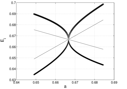
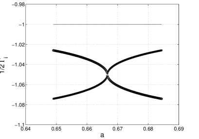
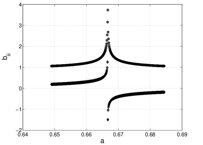
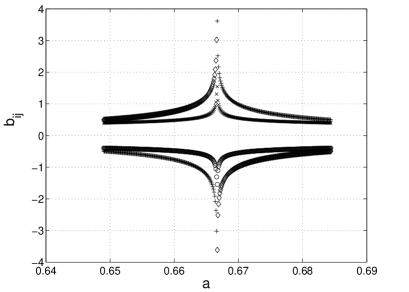
FIG. 1.: The energies $E_{i}$ (top left) and widths $\Gamma_{i}/2$ (top right) of the two eigenstates of the matrix (39) as a function of the parameter $a$. The thin lines give the energies $E_{i}$ and widths $\Gamma_{i}/2$ of the states at $\omega=0$. The lower part of the figure shows the coefficients $b_{ii}$ (bottom left) and $b_{ij\neq i}$ (bottom right) defined by Eq. (42). The x and o denote the $\Re(b_{ij})$ while the $\Im(b_{ij})$ are denoted by + and $\diamond$. $e_{1}=1-a/2;\;e_{2}=a;\;\gamma_{1}/2=1.0;\;\gamma_{2}/2=1.1$ and $\omega=0.05$.

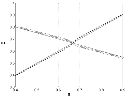
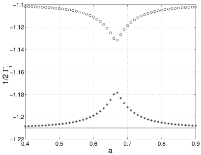
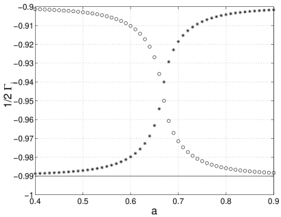
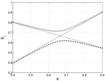
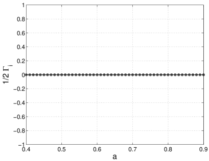
FIG. 2.: The energies $E_{i}$ (left) and widths $\Gamma_{i}/2$ (right) as a function of the tuning parameter $a$. $e_{1}=1-a/2;\;e_{2}=a$ and $\omega=0.05$. The $\gamma_{1}/2$ are 1.10 (top), 0.90 (middle), 0 (bottom); $\gamma_{2}=1.1\cdot\gamma_{1}$. The full lines show the $E_{i}$ and $\Gamma_{i}/2$ for $\omega=0$.

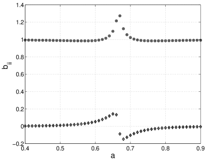
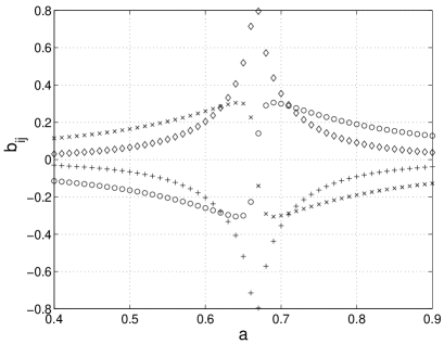
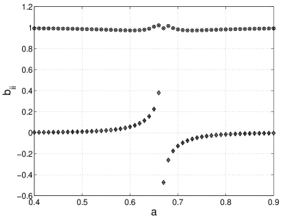
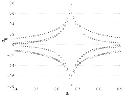
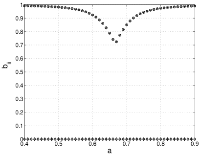
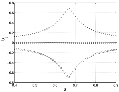
FIG. 3.: The mixing coefficients $b_{ii}$ (left) and $b_{ij\neq i}$ (right) defined by Eq. (42) as a function of the tuning parameter $a$. o and x denote the real parts and $\diamond$ and + the imaginary parts. $e_{1}=1-a/2;\;e_{2}=a$ and $\omega=0.05$. The $\gamma_{1}/2$ are the same as in Fig. 2: 1.10 (top), 0.90 (middle), 0 (bottom); $\gamma_{2}=1.1\cdot\gamma_{1}$. Note the different scales in the three cases.

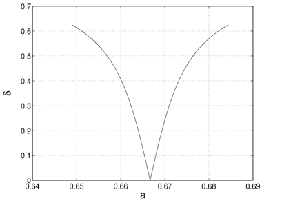
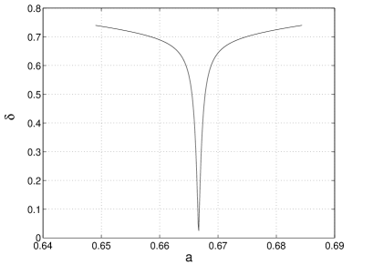
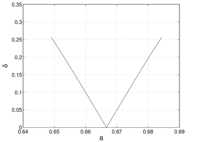
FIG. 4.: The differences $\delta=|b_{ii}|^{2}-|b_{ij\neq i}|^{2}$ as a function of the tuning parameter $a$. $e_{1}=1-a/2;\;e_{2}=a$ and $\omega=0.05$. The $\gamma_{1}/2$ are 1.010 (top left), 0.990 (bottom left), 0.90 (top right), 0 (bottom right); $\gamma_{2}=1.1\cdot\gamma_{1}$. Note the different scales in the different figures.

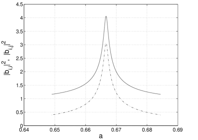
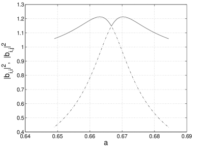
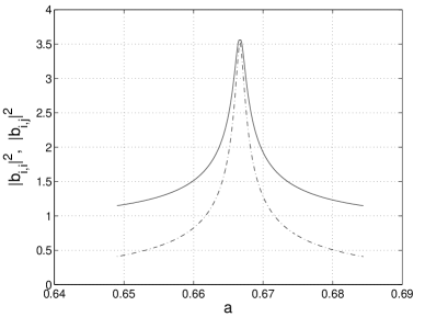
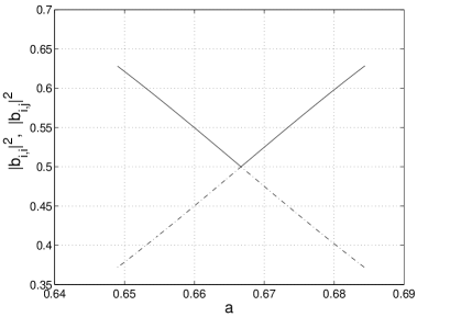
FIG. 5.: The $|b_{ii}|^{2}$ (full lines) and $|b_{ij\neq i}|^{2}$ (dash-dotted lines) as a function of the tuning parameter $a$. $e_{1}=1-a/2;\;e_{2}=a$ and $\omega=0.05$. The $\gamma_{1}/2$ are the same as in Fig. 4: 1.010 (top left), 0.990 (bottom left), 0.90 (top right), 0 (bottom right); $\gamma_{2}=1.1\cdot\gamma_{1}$. Note the different scales in the different figures.

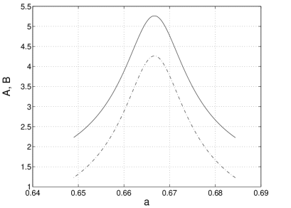
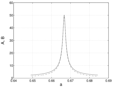
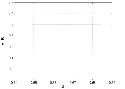
FIG. 6.: The $A$ (full lines) and $B$ (dash-dotted lines) defined in Eq. (23) as a function of the tuning parameter $a$. $e_{1}=1-a/2;\;e_{2}=a$ and $\omega=0.05$. The $\gamma_{1}/2$ are the same as in Fig. 4: 1.010 (top left), 0.990 (bottom left), 0.90 (top right), 0 (bottom right); $\gamma_{2}=1.1\cdot\gamma_{1}$. Note the different scales in the different figures.

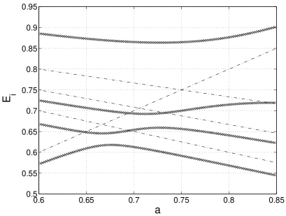
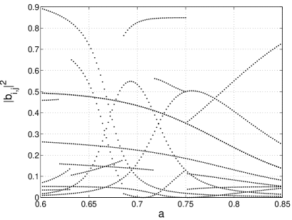
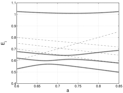
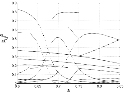
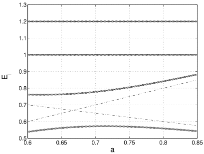
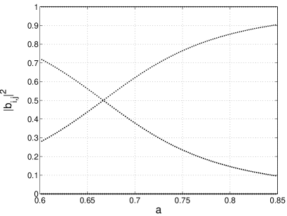
FIG. 7.: The energies $E_{i}$ (left) and mixing coefficients $|b_{ij}|^{2}$ (right) of four discrete states ($\gamma_{i}=0$ for $i=1,...,4$) obtained from ${\cal H}^{(4)}$, Eq. (65), as a function of the tuning parameter $a$. Top and middle: $e_{1}=1-a/3;\;e_{2}=1-5a/12;\;e_{3}=1-a/2;\;e_{4}=a$; $~{}\omega=0.05$ (top) and 0.1 (middle) for all non-diagonal matrix elements. Bottom: the same as above but $e_{1}=1;\;e_{2}=1.2$; $\omega=0$ for the coupling between the states $i=1,2$ and $j\neq i$, $\;\omega=0.1$ for the coupling between $i=3,4$ and $j=4,3$. In this case, $|b_{ii}|^{2}\geq|b_{ij\neq i}|^{2}$ (bottom right) as in Fig. 5 (bottom right). The dash-dotted lines (left) show $E_{i}$ for $\omega=0$. The states $i$ and $j$ are exchanged at some values $a$.

REFERENCES

- [1] V. Zelevinsky, B.A. Brown, N. Frazier, and M. Horoi, Phys. Rep. 276, 85 (1996); V. Zelevinsky, Ann. Rev. Nucl. Part. Sci. 46, 237 (1996)
- [2] C.W. Johnson, G.F. Bertsch and D.J. Dean, Phys. Rev. Lett. 80, 2749 (1998); C.W. Johnson, G.F. Bertsch, D.J. Dean and I. Talmi, Phys. Rev. C 6101, 4311 (2000)
- [3] R. Bijker, A. Frank, and S. Pittel, Phys. Rev. C 6002, 1302 (1999)
- [4] L. Kaplan and T. Papenbrock, Phys. Rev. Lett. 84, 4553 (2000)
- [5] D. Mulhall, A. Volya and V. Zelevinsky, Phys. Rev. Lett. 85, 4016
- [6] S. Drożdż and M. Wójcik, arXiv:nucl-th/0007045
- [7] J. Flores, M. Horoi, M. Müller and T.H. Seligman, Phys. Rev. E 6302, 6204 (2001)
- [8] I. Rotter, E. Persson, K. Pichugin and P. eba, Phys. Rev. E 62, 450 (2000)
- [9] E. Persson, I. Rotter, H.J. Stöckmann and M. Barth, Phys. Rev. Lett. 85, 2478 (2000)
- [10] W.D. Heiss, M. Müller, and I. Rotter, Phys. Rev. E 58, 2894 (1998)
- [11] H.M. Lauber, P. Weidenhammer and D. Dubbers, Phys. Rev. Lett. 72, 1004 (1994)
- [12] D.E. Manolopoulos and M.S. Child, Phys. Rev. Lett. 82, 2223 (1999)
- [13] F. Pistolesi and N. Manini, Phys. Rev. Lett. 85, 1585 (2000)
- [14] J.S. Briggs, V.I. Savichev and E.A. Solov’ev, J. Phys. B 33, 3363 (2000)
- [15] E.A. Solov’ev, Sov. Phys. – JETP 54, 893 (1981); – USP 32, 228 (1989)
- [16] A.I. Magunov, I. Rotter and S.I. Strakhova, J. Phys. B 32, 1669 (1999)
- [17] A.I. Magunov, I. Rotter and S.I. Strakhova, J. Phys. B 34, 29 (2001)
- [18] T. Timberlake and L.E. Reichl, Phys. Rev. A 59, 2886 (1999)
- [19] F. Haake Quantum Signatures of Chaos, Springer, Berlin 1991
- [20] H.W. Barz, J. Höhn and I. Rotter, Nucl. Phys. A 275, 111 (1977)
- [21] I. Rotter, Rep. Progr. Phys. 54, 635 (1991)
- [22] M. Müller, F.M. Dittes, W. Iskra and I. Rotter, Phys. Rev. E 52 5961 (1995)
- [23] E. Persson, T. Gorin and I. Rotter, Phys. Rev. E 54, 3339 (1996) and 58, 1334 (1998)
- [24] S. Drożdż, J. Okołowicz, M. Płoszajczak, and I. Rotter, Phys. Rev. C 62, 024313 (2000)
- [25] H.J. Stöckmann et al., to be published
- [26] F.M. Dittes, Phys. Rep. 339, 215 (2000)
- [27] R.G. Nazmitdinov, K.N. Pichugin, I. Rotter and P. eba, arXiv:cond-mat/0104056
- [28] C. Mahaux and H.A. Weidenmüller Shell-model approach to nuclear reactions, Springer, Berlin 1969
- [29] R.G. Newton, Scattering Theory of Waves and Particles, Springer, New York 1982
- [30] W. Iskra, M. Müller and I. Rotter, J. Phys. G 19, 2045 (1993) and 20, 775 (1994)
- [31] E. Persson, K. Pichugin, I. Rotter and P. eba, Phys. Rev. E 58, 8001 (1998)
- [32] P. eba, I. Rotter, M. Müller, E. Persson and K. Pichugin, Phys. Rev. E 61, 66 (2000)