Quantum State Tomography of Complex Multimode Fields using Array Detectors

Abstract

We demonstrate that it is possible to use the balanced homodyning with array detectors to measure the quantum state of correlated two-mode signal field. We show the applicability of the method to fields with complex mode functions, thus generalizing the work of Beck(Phys. Rev. Lett. 84, 5748 (2000)) in several important ways. We further establish that, under suitable conditions, array detector measurements from one of the two ouputs is sufficient to determine the quantum state of signal. We show the power of the method by reconstructing a truncated Perelomov state which exhibits complicated structure in the joint probability density for the quadratures.

I Introduction

The subject of quantum state tomography (QST) has been of great interest in the recent years after the experimental reconstruction of the complete wave function of the vacuum and squeezed states by balanced homodyne (BHD) method[1, 2, 3]. Much progress has been made by way of theoretical exploration of alternate schemes of QST like the self-homodyne tomography and their experimental verification[4]. In essence, the BHD method combines a strong local oscillator (LO) with the signal in a 50:50 beam-splitter (BS). The two outputs of the BS are measured by two photodetectors and electronically subtracted. The resultant quantity is directly proportional to the rotated quadrature $[\hat{a}\exp(-i\phi)+\hat{a}^{\dagger}\exp(i\phi)]/\sqrt{2}$ of the signal field and the angle $\phi$ is fixed by the LO. By performing the experiment many times for a given $\phi$ and repeating it for various values of $\phi$ in the range of $0\leq\phi\leq\pi$, the probability density $p(x,\phi)$ for the quadrature rotated through $\phi$ can be measured. From the measured probability density the Wigner function for the signal can be constructed and hence the elements of the density matrix[5, 6]. The serious problems that may arise in the numerical reconstruction of density matrix elements and the methods to avoid such pitfalls are discussed in the review article by Welsch et al [6] and in Ref. [7]. The BHD can be extended [8, 9, 10, 11, 12] to multimode signals and to measure other distributions like the positive P-distribution. The BHD is for optical fields and methods have been developed for reconstructing the vibrational state of molecules[13] and spin systems[14]. For measruing the quantum states of the modes of a cavity, atoms with properly chosen energy levels can be used as probes [15].

A serious drawback of the BHD using single detectors is the requirement for mode matching the signal and LO mode functions. A quantitative measure of mode matching is the overlap between the signal and LO mode functions and the efficiency of the BHD scheme is directly proportional to it,

$${\rm efficiency}\propto\int U^{*}_{\rm signal}(x)U_{\rm LO}(x)dx.$$ (1)

Here $U_{\rm signal}$ and $U_{\rm LO}$ are the respective mode functions of the signal and LO. If there is perfect mode matching, i.e., the overlap integral is unity, the BHD is very efficient. In the case of signal and the LO modes being orthogonal to each other, the BHD simply fails to determine the quantum state of the signal.

An ingenious way of circumventing the problem of mode matching was suggested by Beck[16]. The key idea is to replace the single detectors at the BS output ports by array detectors. Beck considers array detectors with pixels small enough such that the mode functions of the LO and signal over any pixel is constant. The output from a given pixel labeled $(j,j^{\prime})$ of one of the array detectors is given by

$$N_{1}(j,j^{\prime},\phi)={{\delta x\delta ycT}\over{2L}}\Big{[}{|\beta|^{2}\over{D_{x}D_{y}}}+\sum_{n,m}\hat{a}^{\dagger}_{n}\hat{a}_{m}U^{*}_{n}(j,j^{\prime})U_{m}(j,j^{\prime})$$ (2)

$$+{\beta\over{\sqrt{D_{x}D_{y}}}}\sum_{m}[\hat{a}_{m}\exp(-i\phi)U_{m}(j,j^{\prime})+H.c]\Big{]}.$$ (3)

Here the signal is taken to be multimode and the LO is assumed to be a single mode coherent state $|\beta\exp^{i\phi}\rangle$ ($\beta$ real). The summation is over the various modes of the signal field. The function $U_{m}(j,j^{\prime})$ is the value of the $m$th mode function of the signal over the pixel $(j,j^{\prime})$. The operators $\hat{a}^{\dagger}_{m}$ and $\hat{a}_{m}$ are the creation and annihilation operators for the $m$th mode of the signal. The mode function for the LO is taken to be the constant $1\over{\sqrt{D_{x}D_{y}}}$ over the entire detector surface. The dimension of each pixel is $\delta x\times\delta y$ and that of the detector is $D_{x}\times D_{y}$ (=$N\delta x\times N\delta y$). The constant $c$ is the speed of light vacuum, $T$ is the duration of counting and $L$ is the longitudinal quantization length. Similarly, the output of the corresponding pixel at the other output port of BS is given by

$$N_{2}(j,j^{\prime},\phi) = {{\delta x\delta ycT}\over{2L}}\Big{[}{|\beta|^{2}\over{D_{x}D_{y}}}+\sum_{n,m}\hat{a}^{\dagger}_{n}\hat{a}_{m}U^{*}_{n}(j,j^{\prime})U_{m}(j,j^{\prime})$$ (5)

$$-{\beta\over{\sqrt{D_{x}D_{y}}}}\sum_{m}[\hat{a}_{m}\exp(-i\phi)U_{m}(j,j^{\prime})+H.c]\Big{]}.$$

On taking the difference of $N_{1}(j,j^{\prime},\phi)$ and $N_{2}(j,j^{\prime},\phi)$, it is seen that

$$N_{d}(j,j^{\prime},\phi)={{\delta x\delta y}\over{\sqrt{D_{x}D_{y}}}}\beta\sum_{m}[\hat{a}_{m}\exp(-i\phi)U_{m}(j,j^{\prime})+H.c],$$ (6)

where we have set $L=cT$. If one of the mode functions, say $U_{l}$, is real, then the above expression yields, on summing over all the pixel indices and using orthonormal relationship among the modes,

$$\sum_{j,j^{\prime}}N_{d}(j,j^{\prime},\phi)U_{l}(j,j^{\prime})={1\over{\sqrt{D_{x}D_{y}}}}\beta[\hat{a}_{l}\exp(-i\phi)+\hat{a}^{\dagger}_{l}\exp(i\phi)].$$ (7)

It is to be noted that the mode matching factor does not enter in the expression relating the measured photocurrent difference and the rotated quadrature. This is of great practical utility as mode matching is extremely difficult in an actual experiment. The above expression for quadrature works for any mode function that is real and hence the quantum state of all such modes can be determined. However, their joint state cannot be estimated by the method as proposed by Beck. But correlated quantum states are of prime importance for conceptual understanding of quantum theory as well as applications[17, 18]. Hence, it is all the more essential that the array detector scheme be extended to correlated multimode fields whose mode functions need not be real.

In the present work we extend the Beck’s method to two-mode correlated states by interposing a linear device which introduces a variable relative phase between the two modes. The stringent condition to have real mode functions is relaxed by making measurements with the LO phase varying from zero to $3{\pi\over 2}$ and combining the measurements to get the value of the quadratures roatated through zero to $\pi$ as required for state reconstruction. Further, we establish that one of the outputs of BS as measured by an array detector is sufficient to measure the quantum state. This paper is organized as follows. In Section II the extension of Beck’s work to two-mode correlated state is given. Section III of the paper contains the results of Monte Carlo simulations to demonstrate the power of the method to construct joint probability densities with complicated structures. In Section IV of the paper we explicitly show that for mode functions satisfying certain conditions, a single array detector is sufficient to measure the quantum state. We have provided an appendix to make transparent the arguments given Section II for realxing the requirement for real mode functions.

II Joint quantum state of two-mode field

In the present section a method of estimating the quantum state of a correlated two mode signal is given. The basic requirement is to construct the joint probability density $P(x_{1},\phi_{1},x_{2},\phi_{2})$ for the two quadratures rotated through $\phi_{1}$ and $\phi_{2}$ respectively. It is, therefore, essential to rotate the two quadratures independently. If the signal modes are spatially seperable, they can be mixed with two independent LOs (usually made from a single source by using a BS) and measurements are carried out using two BHD arrangements[4]. In the other case, the signal is passed through a medium which mixes the modes with a relative phase. The mixed modes are taken to be spatially seperable[9] and one of the seperated modes is used in the input port of BS. This requires only one LO and one BHD arrangment. In both the cases, however, spatial seperation of modes is required at some stage and mode matching is essential. In the present section we discuss how to use the BHD with array detectors in the latter method. The mixing of modes is achieved by using a linear device which introduces a relative phase between the two modes. For instance, the linear device could be a medium in which the two modes interact via the Hamiltonian given by

$$H_{int}\propto\hat{a}^{\dagger}_{1}\hat{a}_{2}\exp(i\theta)+H.c$$ (8)

The field operators $(\hat{a}_{1}^{\prime},\hat{a}^{\prime}_{2})$ at the output of the linear device can be written as

$$\hat{a}^{\prime}_{1} = {\cos\nu}\hat{a}_{1}-i{\sin\nu}\exp(-i\theta)~{}\hat{a}_{2},$$ (9)

$$\hat{a}^{\prime}_{2} = {\cos\nu}\hat{a}_{2}-i{\sin\nu}\exp(i\theta)~{}\hat{a}_{1},$$ (10)

where $\nu$ is a constant determined by the length of the linear device, strength of interaction, etc. The device mixes the two modes of the signal. For later use we define the rotated quadratures for the transformed field:

$$\hat{X}^{\prime}_{k}(\phi,\theta,\nu)={\hat{a}^{\prime}_{k}\exp(-i\phi)+\hat{a}^{\dagger\prime}_{k}\exp(i\phi)\over\sqrt{2}},~{}~{}~{}~{}k=1,2$$ (11)

The positive frequency part of the electric field operator entering the signal port of BS is

$$\hat{E}^{(+)^{\prime}}(x,y)=\Big{[}{2\pi\hbar\tilde{\omega}\over L}\Big{]}^{1/2}\left[U_{1}(x,y)\hat{a}^{\prime}_{1}+U_{2}(x,y)\hat{a}^{\prime}_{2}\right].$$ (12)

The electric field operator depends on $\phi$,$\theta$ and $\nu$ in addition to the spatial coordinates $(x,y)$. However, in the sequel we include the dependence explicitly in the expressions for difference counts and other derived quantities. With the field operators given by Eq.9 entering the signal port of BS and the LO phase fixed at $\phi$, the difference count $N_{d}(j,j^{\prime},\phi,\theta,\nu)$ is

$$N_{d}(j,j^{\prime},\phi,\theta,\nu) = \beta{\delta x\delta y\over{\sqrt{D_{x}D_{y}}}}\Big{[}\exp(-i\phi)[U_{1}(j,j^{\prime})\hat{a}^{\prime}_{1}+U_{2}(j,j^{\prime})\hat{a}^{\prime}_{2}]$$ (14)

$$+\exp(i\phi)[U_{1}^{*}(j,j^{\prime})\hat{a}^{\dagger\prime}_{1}+U_{2}^{*}(j,j^{\prime})\hat{a}^{\dagger\prime}_{2}]\Big{]}.$$

and the difference count with the LO phase rotated further by $\pi/2$ is

$$N_{d}(j,j^{\prime},\phi+{\pi\over 2},\theta,\nu) = i\beta{\delta x\delta y\over{\sqrt{D_{x}D_{y}}}}\Big{[}\exp(i\phi)[U_{1}^{*}(j,j^{\prime})\hat{a}^{\dagger\prime}_{1}+U_{2}^{*}(j,j^{\prime})\hat{a}^{\dagger\prime}_{2}]$$ (16)

$$-\exp(-i\phi)[U_{1}(j,j^{\prime})\hat{a}^{\prime}_{1}+U_{2}(j,j^{\prime})\hat{a}^{\prime}_{2}]\Big{]}.$$

The quantities $N_{d}(j,j^{\prime},\phi,\theta,\nu)$ and $N_{d}(j,j^{\prime},\phi+{\pi\over 2},\theta,\nu)$ are measured in the experiment. From these measured quantities we construct

$$R(j,j^{\prime},\phi,\theta,\nu) = {1\over{2\beta}}\sqrt{D_{x}D_{y}\over{2}}\{N_{d}(j,j^{\prime},\phi,\theta,\nu)$$ (18)

$${}-iN_{d}(j,j^{\prime},\phi+{\pi\over{2}},\theta,\nu)\},$$

$$= {\delta x\delta y\over{\sqrt{2}}}\exp(i\phi)[\hat{a}^{\dagger\prime}_{1}U^{*}_{1}(j,j^{\prime})+\hat{a}^{\dagger\prime}_{2}U^{*}_{2}(j,j^{\prime})].$$ (19)

Multiplying $R(j,j^{\prime},\phi,\theta,\nu)$ by $U_{k}(j,j^{\prime})$ $(k=1,2)$ and summing over $(j,j^{\prime})$ yields

$$\sum_{j,j^{\prime}}R(j,j^{\prime},\phi,\theta,\nu)U_{k}(j,j^{\prime}) = {1\over{\sqrt{2}}}\exp(i\phi)\hat{a}^{\dagger\prime}_{k}.$$ (20)

The quadrature $\hat{X}{{}^{\prime}}_{k}(\phi)$ can now be written in terms $R(j,j^{\prime},\phi,\theta,\nu)$ and its conjugate as

$$X{{}^{\prime}}_{k}(\phi)=\sum_{j,j^{\prime}}[R(j,j{{}^{\prime}},\phi,\theta,\nu)U_{k}(j,j^{\prime})+C.c].$$ (21)

The equations determine the mixed quadratures in terms of measured difference counts. Using Eqs. 9-10, the quadratures for the mixed mode can be written in terms of the signal quadratures as

$$\hat{X}{{}^{\prime}}_{1}(\phi,\theta,\nu) = \cos\nu\hat{X}_{1}(\phi)+\sin\nu\hat{X}_{2}(\phi+\theta+{\pi\over 2}),$$ (22)

$$\hat{X}{{}^{\prime}}_{2}(\phi,\theta,\nu) = \cos\nu\hat{X}_{2}(\phi)+\sin\nu\hat{X}_{1}(\phi-\theta+{\pi\over 2}).$$ (23)

If measurements are carried out for two values of $\nu$, say $\nu_{1}$ and $\nu_{2}$, then the signal quadratures can be evaluated from Eqs.(22)-(23) and the resulting expressions are:

$$\hat{X}_{2}(\phi) = {1\over{\sin(\nu_{2}-\nu_{1})}}[\sin\nu_{1}\hat{X}{{}^{\prime}}_{2}(\theta,\phi,\nu_{2})-\sin\nu_{2}\hat{X}{{}^{\prime}}_{2}(\theta,\phi,\nu_{1})],$$ (24)

$$\hat{X}_{1}(\phi-\theta+{\pi\over{2}}) = {1\over{\sin(\nu_{1}-\nu_{2})}}[\cos\nu_{1}\hat{X}{{}^{\prime}}_{2}(\theta,\phi,\nu_{2})-\cos\nu_{2}\hat{X}{{}^{\prime}}_{2}(\theta,\phi,\nu_{1})],$$ (25)

$$\hat{X}_{1}(\phi) = {1\over{\sin(\nu_{2}-\nu_{1})}}[\sin\nu_{1}\hat{X}{{}^{\prime}}_{1}(\theta,\phi,\nu_{2})-\sin\nu_{2}\hat{X}{{}^{\prime}}_{1}(\theta,\phi,\nu_{1})],$$ (26)

$$\hat{X}_{2}(\phi+\theta+{\pi\over{2}}) = {1\over{\sin(\nu_{1}-\nu_{2})}}[\cos\nu_{1}\hat{X}{{}^{\prime}}_{1}(\theta,\phi,\nu_{2})-\cos\nu_{2}\hat{X}{{}^{\prime}}_{1}(\theta,\phi,\nu_{1})].$$ (27)

The first two expressions yield the values of the quadratures $\hat{X_{2}}$ and $\hat{X_{1}}$ rotated through angles $\phi$ and $\phi-\theta+{\pi\over 2}$ respectively. The last two yield the value of two quadratures rotated through $\phi_{1}=\phi$ and $\phi_{2}=\phi+\theta+{\pi\over{2}}$. By changing the LO phase $\phi$ and the phase $\theta$ in the interaction Hamiltonian, the quadratures can be measured to construct the joint probability distribution $P(x_{1},\phi_{1},x_{2},\phi_{2})$. Note that there is no need to assume that the mode functions are real. Of course, the difference count measurements are to be carried out over a range of $0-3\pi/2$ for the LO phase; in the case of real mode functions it is sufficient to measure the difference count when the LO phase is varied from $0-\pi$. From the measured joint probability density, the Wigner function for the two-mode state can be constructed which, in turn, can be used to determine the density matrix. The measured joint probability can also be used to construct the elements of the density matrix in two-mode number state basis[19].

The scheme suggested here is similar to what is described as the method of generalized rotation in phase space[9]. However, in our scheme there is no need to spatially separate the signal modes at the output of the linear device. This is possible as mode matching is not essential in the present scheme. In fact, not separating them is useful to reduce the number of experimental runs. In one run of the experiment, the pairs $\{\hat{X}_{1}(\phi),\hat{X}_{2}(\phi+\theta+{\pi\over 2})\}$ and $\{\hat{X}_{1}(\phi-\theta+{\pi\over 2}),\hat{X}_{2}(\phi)\}$ are simultaneously estimated.

III Monte Carlo Simulations

In this section we study the experimental feasibility of the above method by Monte Carlo (MC) simulations with the signal in the two-mode Perelomov state[20]. This state is generated from the two-mode vacuum $|0,0\rangle$ as follows:

$$|\zeta\rangle=\exp(\zeta\hat{a}^{\dagger}_{1}\hat{a}^{\dagger}_{2}-\zeta^{*}\hat{a}_{1}\hat{a}_{2})|0,0\rangle.$$ (28)

The number state expansion for the above state is given by

$$|\zeta\rangle={1\over{\cosh r}}\sum_{n=0}^{\infty}[\exp(-i\gamma)\tanh r]^{n}|n,n\rangle,$$ (29)

and the joint probability density is

$$p(x_{1},\phi_{1},x_{2},\phi_{2})={2\over{\pi{\rm AB}}}\exp\Big{[}-{(x_{1}+x_{2})^{2}\over{\rm A}}-{(x_{1}-x_{2})^{2}\over{\rm B}}\Big{]}.$$ (30)

The constants $r$, $\rm A$ and $\rm B$ are related to the squeeze parameter $\zeta$:

$$\zeta = r\exp(-i\gamma),$$ (31)

$$A = {|1+\tanh r\exp[-i(\phi_{1}+\phi_{2}+\gamma)]|^{2}\over{1-\tanh^{2}r}}$$ (32)

$$B = {|1-\tanh r\exp[-i(\phi_{1}+\phi_{2}+\gamma)]|^{2}\over{1-\tanh^{2}r}};$$ (33)

Random numbers distributed according to the distribution given in Eq. 30 were generated from Gaussian distributed random numbers by von Neumann’s rejection method[21]. These numbers were then used to generate the output of an actual experiment. In Fig. 1 the result of the simulation to reconstruct the joint probability density is given for $\phi_{1}=\pi/4$, $\phi_{2}=\pi/2$, $\gamma=\pi/4$ and $r=1.0$ along with its contour plot . For comparison, the theoretical distribution is also given. We find that to reconstruct the probability density with reasonable accuracy, as many as $1.6\times 10^{5}$ experimental runs would be required for each set of values of $\phi_{1}$ and $\phi_{2}$. In Fig. 2 we present the simulated results for identical values for the parameters except $\phi_{2}$ which is set equal to $-\pi/4$. In Fig. 1 the distribution is narrower compared to what is shown in Fig, 2. As expected, from the figures it is clear that the reconstruction is better, for a given number of experiments, if the probability density is narrower.

In order to see whether an experiment can capture the complicated spatial structures of probability density, the MC simulations were done for the signal in truncated Perelomov state. These are defined as

$$|c_{1},c_{2}\rangle=c_{1}|0,0\rangle+c_{2}\exp(-i\delta)|1,1\rangle.$$ (34)

The superposition coefficients $c_{1}$ and $c_{2}$ are taken to be real and they satisfy the normalization condition $c_{1}^{2}+c_{2}^{2}=1$. The joint probability density for the quadratures is

$$p(x_{1},\phi_{1},x_{2},\phi_{2})={\exp{(-x_{1}{{}^{2}}-x_{2}{{}^{2}})}\over\pi}[c_{1}^{2}+4c_{2}^{2}x_{1}{{}^{2}}x_{2}{{}^{2}}+4x_{1}x_{2}c_{1}c_{2}\cos(\phi_{1}+\phi_{2}+\delta)].$$ (35)

The result of the MC simulation for the truncated Perelomov state is depicted in Fig. 3. We have used $c_{1}=c_{2}={1/\sqrt{2}}$, $\delta=\pi/8$, $\phi_{1}=\pi/4$ and $\phi_{2}=\pi/4$. It requires $2\times 10^{5}$ points to generate the pattern shown.

IV QST using a single array detector

In this section we describe how to measure the joint probability density of a two-mode state using an array detector in one of the output ports of BS. No measurements are made at the other output. In the discussions to follow the pixels are labeled by a single index instead of two indices. We first introduce some notations to simplify the expressions:

$$U_{1}(k) : \textrm{value of the mode function $U_{1}$ on the pixel labeled $k$},$$ (36)

$$U_{2}(k) : \textrm{value of the mode function $U_{2}$ on the pixel labeled $k$},$$ (37)

$$n_{d}(k) : 1 k (k=2,3...9)$$ difference count between the pixels labeled and   (38)

$$V^{T} : V$$ transpose of vector whose elements are (41)

$$\{\hat{a}^{\dagger\prime}_{1}\hat{a}^{\prime}_{1},\quad\hat{a}^{\dagger\prime}_{2}\hat{a}^{\prime}_{2},\quad\hat{a}^{\dagger\prime}_{1}\hat{a}^{\prime}_{2},\quad\hat{a}^{\prime}_{1}\hat{a}^{\dagger\prime}_{2},\quad\exp(-i\phi)\hat{a}^{\prime}_{1},\quad\exp(i\phi)\hat{a}^{\dagger\prime}_{1},$$

$$\quad\exp(-i\phi)\hat{a}^{\prime}_{2},\quad\exp(i\phi)\hat{a}^{\dagger\prime}_{2}\}$$

$$M : 8\times 8 (k-1) (k=2,..9)$$ an matrix whose th row is given by (46)

$$\{U^{2}_{1}(1)-U^{2}_{1}(k),\quad U^{2}_{2}(1)-U^{2}_{2}(k),\quad U^{*}_{1}(1)U_{2}(1)-U^{*}_{1}(k)U_{2}(k),$$

$$U_{1}(1)U^{*}_{2}(1)-U_{1}(k)U^{*}_{2}(k),\quad S[U_{1}(1)-U_{1}(k)],$$

$$S[U^{*}_{1}(1)-U^{*}_{1}(k)],\quad S[U_{2}(1)-U_{2}(k)],\quad S[U^{*}_{2}(1)-U^{*}_{1}(k)]\},$$

$${}\textrm{where}~{}~{}S={\beta\over\sqrt{D_{x}D_{y}}}$$

The expression for $n_{d}(k)~{}(k=2,3\cdot\cdot\cdot 9)$ is

$$n_{d}(k) = k$$ Counts in pixel 1 - Counts in pixel (47)

$$= {\delta x\delta y\over 2}\Big{[}\sum_{n,m=1}^{2}\hat{a}^{\dagger\prime}_{n}\hat{a}^{\prime}_{m}[U^{*}_{n}(1)U_{m}(1)-U^{*}_{n}(k)U_{m}(k)]$$ (49)

$${}+{\beta\over{\sqrt{D_{x}D_{y}}}}\sum_{m}[\exp(-i\phi)\hat{a}^{\prime}_{m}[U_{m}(1)-U_{m}(k)]+H.c]\Big{]}$$

$$= {\delta x\delta y\over 2}\sum_{j=1}^{8}M_{kj}V_{j}.$$ (50)

The elements of the matrix are various combinations of the mode functions $U_{1}$ and $U_{2}$ over a selected set of nine pixels of the array detector. If the elements of $M$ are such that the matrix is invertible, the elements of the vector $V$ can be determined from the equation

$$V_{j}=\sum_{k=2}^{9}(M^{-1})_{j,k-1}n_{d}(k)\quad j=1,2\cdot\cdot\cdot 8.$$ (51)

Note that the vector $V$ has as its elements the creation and annihilation operators of the two modes and their quadratic forms. The above equation then implies that the elements of $V$ are determined from the measured quantities $n_{d}(k)$. It is evident that the mixed quadratures can be determined as

$$\hat{X}{{}^{\prime}}_{1}(\phi,\theta,\nu) = {V_{5}+V_{6}\over\sqrt{2}},$$ (52)

$$\hat{X}{{}^{\prime}}_{2}(\phi,\theta,\nu) = {V_{7}+V_{8}\over\sqrt{2}}.$$ (53)

Once the mixed quadratures are estimated, the signal mode qudratures are obtained using Eqs.22-23. It is clear that if we can choose nine pixels so that the matrix $M$ is invertible, then the joint probability density of two-mode states can be determined. Despite the fact that only one of the output ports of BS is used, the LO fluctuations are eliminated as in the case of BHD. Another interesting feature is that there is no need to assume that the mode functions are real and the LO phase need not be changed beyond the usual range $0-\pi$. The method can be extended to more than two modes. But the requirements on the mode functions will become more stringent.

V Summary

The use of array detectors in BHD eliminates the need for difficult-to-achieve mode-matching. For two-mode signals, a linear device to introduce a relative phase between two modes can be used in the signal port of the BS. By varying the LO phase from zero to $3\pi\over 2$ and the relative phase between the modes, the joint probability density for the quadratures of the two modes can be experimentally determined. The QST measurements can carried out with one array detector instead of detectors at both the output ports of BS. The method retains the advantage of BHD in the sense that the LO fluctuations do not affect the measurement. However, the success of the method depends of the shape of the mode functions.

A QST of a single, complex mode signal

In this appendix we show how to measure the quantum state of a single, complex mode signal. This appendix is provided to make the arguments of Section II more transparent. In Beck’s method it is required to have the mode function real for determining its quantum state. If the mode function is not real, then it cannot be factored out in the RHS of Eq. (6) and hence the measured difference count cannot be related to the quadrature. Note that this problem does not arise in the case of the conventional BHD using single detectors. We set $N_{d}(j,j^{\prime},\phi)$ as $N_{d}(\phi)$ and $U(j,j^{\prime})$ as $U$ to avoid lengthy expressions. Hence, Eq. (6) is rewritten as

$$N_{d}(\phi)={{\delta x\delta y}\over{\sqrt{D_{x}D_{y}}}}\beta[U\exp(-i\phi)\hat{a}+U{{}^{*}}\exp(i\phi)\hat{a}^{\dagger}].$$ (A1)

With the LO phase rotated through $\phi+{\pi\over 2}$, the difference count is

$$N_{d}(\phi+{\pi\over 2})=i{{\delta x\delta y}\over{\sqrt{D_{x}D_{y}}}}\beta[\hat{a}^{\dagger}\exp(i\phi)U{{}^{*}}-U\exp(-i\phi)\hat{a}].$$ (A2)

Comibining the expressions for $N_{d}(\phi)$ and $N_{d}(\phi+{\pi\over 2})$ we get

$$N_{d}(\phi)-iN_{d}(\phi+{\pi\over 2})=U{{}^{*}}\exp(i\phi)\hat{a}^{\dagger}$$ (A3)

and

$$N_{d}(\phi)+iN_{d}(\phi+{\pi\over 2})=U\exp(-i\phi)\hat{a}.$$ (A4)

Having measured the operators $\exp(-i\phi)\hat{a}$ and its adjoint, the quadrature can be estimated at once as it is a linear combination of the two operators. To achieve this we multiply the last two equations by $U$ and $U{{}^{*}}$ respectively and use the normalization relation $\delta x\delta y\sum_{j.j^{\prime}}U^{*}U=1$ to yield

$$\hat{X}(\phi)={\sqrt{D_{x}D_{y}}\over{2\sqrt{2}\beta}}\sum_{j,j^{\prime}}[N_{d}(\phi)(U+U^{*})+iN_{d}(\phi+{\pi\over 2})(U^{*}-U)].$$ (A5)

As asserted in the beginning of the appendix, there is no need to assume the mode functions to be real in the above expression. When $U$ is real the second term on the RHS vanishes and we recover, as expected, Eq.7.

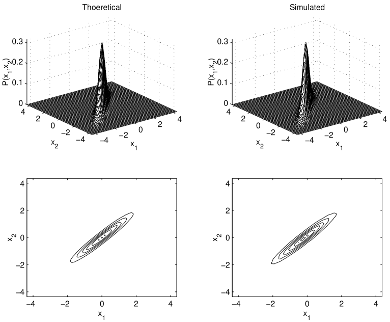
FIG. 1.: Joint probability density for two-mode Perelomov state. The parameter values are $\phi_{1}=\pi/4$, $\phi_{2}=\pi/2$, $\gamma=\pi/4$ and $r=1.0$.

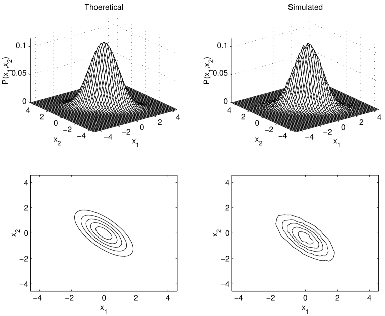
FIG. 2.: Joint probability density for two-mode Perelomov state with with the parameters taking the same values as in Fig. 1 except $\phi_{2}$ which is set equal to $-\pi/4$.

FIG. 3.: Theoretical and simulated joint probability densities for the truncated Perelomov state. The parameter values are $c_{1}=c_{2}=1/\sqrt{2}$ and $\delta=\pi/8$

REFERENCES

- [1] D.T. Smithey, M.Beck, M.G. Raymer, and A. Faridani, Phys. Rev. Lett. 70, 1244 (1993).
- [2] D.T.Smithey, M. Beck, J. Cooper, and M.G. Raymer, Phys. Rev. A 48, 3159 (1993).
- [3] G. Breitenbach, T. Muller, S.F. Pereira, J.-Ph. Poziat, S. Schiller, and J. Mlynek, J. Opt. Soc. Am. B, 12, 2304 (1995).
- [4] M. Vasilyev, S.-K. Choi, P. Kumar and G.M. D’Ariano, Phys. Rev. Lett. 84, 2354 (2000).
- [5] K. Vogel, and H. Risken, Phys. Rev. A 40, 2847 (1989).
- [6] For review see: U. Leonhardt, Measuring the Quantum State of Light, Oxford University Press, Oxford (1997); D.-G. Welsch, W. Vogel, and T. Opantry,Progress in Optics, Ed. E. Wolf, Vol. XXXIX (1999).
- [7] G. S. Agarwal and J. Banerjee, LANL e-print quant-ph 0007049 (submitted to Phys. Rev. A.)
- [8] M.G. Raymer, D.F. McAlister, and U. Leonhardt, Phys. Rev. A. 54, 2397 (1996).
- [9] M.G. Raymer, and A.C. Funk, Phys. Rev. A. 61, 015801 (1999).
- [10] T. Opantry, D.-G. Welsch, and W. Vogel, Phys. Rev. A 55, 1416 (1997).
- [11] C. Iaconis, E. Mukamel, and I. A. Walmsley J. Opt. B 2, 510 (2000).
- [12] G. S. Agarwal and S. Chaturvedi, Phy. Rev. A 49, R665(1994).
- [13] T. J. Dunn, J. N. Sweetser, I. A. Walmsley, and C. Radzewicz, Phys. Rev. Lett. 70, 3388 (1993); T. J. Dunn, I. A. Walmsley, and S. Mukamel, ibid. 74, 884 (1995).
- [14] G. S. Agarwal, Phy. Rev. A 57, 671(1998).
- [15] M. S. Kim and G. S. Agarwal, Phy. Rev. A 59, 3044 (1999).
- [16] M. Beck, Phys. Rev. Lett. 84, 5748 (2000).
- [17] Z. -Y. Ou and L. Mandel, Phys. Rev. Lett 61, 50 (1988); Y. H. Shih and C. O. Alley, Phys. Rev. Lett. 61, 2921 (1988).
- [18] D. Bouwmeester, J. -W. Pan, K. Mattle, M. Eibl, H. Weinfurter, and A. Zeilinger, Nature (London) 390, 575 (1997); D. Boschi, S. Branca, F. De Martini, L. Hardy, and S. Popescu, Phys. Rev. Lett. 80, 1121 (1998); A. Furusawa, J. L. Sorensen, S. L. Braunstein, C. A. Fuchs, H. J. Kimble, and E. S. Polzik, Science 282, 706 (1998).
- [19] G. M. D’Ariano, U. Leonhardt, and H. Paul, Phys. Rev. A 52, R1801 (1995).
- [20] B. Schumaker and C. M. Caves, Phys. Rev. A 31, 3093 (1985).
- [21] W. H. Press, S. A. Teukolsky, W. T. Vettering, and B. P. Flannery, Numerical Recipes in FORTRAN, Cambridge University Press (1995).