Abstract

The maximum-likelihood method for quantum estimation is reviewed and applied to the reconstruction of density matrix of spin and radiation as well as to the determination of several parameters of interest in quantum optics.

1 Introduction

Quantum estimation of states, observables and parameters is, from very basic principles, matter of statistical inference after sampling a population. Why is it so ? And what does this statement exactly mean ? The quantum description of a physical system is intrinsically a statistical one since given an unknown quantum state $\hat{\varrho}\,$: i) one cannot determine the quantum state from a single measurement (even joint measurement) performed on the system [1]; ii) it is not possible to measure different observables after copying the state preparation at disposal, since the linearity of quantum mechanics leads to the impossibility of cloning an arbitrary state [2]. In a way, this means that any quantum estimation procedure necessary requires many identical preparations of the system under examination, on which one performs repeated measurements of an observable or of a set of observables.

The full inference of the quantum state from feasible measurements is a hot topic of the last decade. In recent years, experiments have been performed to characterize the quantum state of different physical systems, such as single-mode radiation field [3], a diatomic molecule [4], a trapped ion [5], and an atomic beam [6]. These results stimulated some efforts for efficient data-processing algorithms, in order to extract the maximum available information on the quantum state, since one always deals with finite ensembles [7], and every detection scheme is affected by noise and imperfections. The need for an efficient data processing is even more stringent in cases where one is not interested in the complete characterization of the state, but only in some specific feature, as when one addresses the problem of characterizing a device, rather than a quantum state, as, for example, the estimation of coupling constants, gain coefficients, or nonlinear susceptibilities.

The most comprehensive quantum estimation procedure is quantum tomography [8]. In quantum tomography the expectation value of an operator is obtained by averaging a special function (usually termed sampling kernel or pattern function) over the experimental data of a sufficiently complete set of observables which is called a “quorum”. For example, in homodyne tomography of radiation the quorum observables are the quadratures of the e.m. field (for varying phase with respect to the local oscillator). The expectation value of a generic operator is obtained by averaging the corresponding pattern function over data. The method is very general and efficient, however, in the averaging procedure, we have fluctuations which result in large statistical errors.

In this paper we review the the maximum-likelihood (ML) principle approach to the quantum estimation problem. The ML idea is to find the quantum state, or the value of the parameters, that are most likely to generate the observed data. This idea can be quantified and implemented using the concept of the likelihood functional. Concerning the estimation of quantum state, in contrast to quantum tomography, the ML method estimates the state as a whole. As a result, a priori knowledge about properties of the density matrix can be incorporated from the very beginning, thus assuring positivity and normalization of matrix, with the result of a substantial reduction of statistical errors [9]. Regarding the estimation of specific parameters, we notice that in all the cases here analyzed the resulting estimators are efficient, unbiased and consistent, thus providing a statistically reliable determination [10]. Moreover, by using the ML method only small samples of data are required for a precise determination.

2 Maximum likelihood principle

Here we briefly review the theory of the maximum-likelihood (ML) estimation of a single parameter. The generalization to several parameters, as for example the elements of the density matrix is, in principle, straightforward. The only point that should be carefully analyzed is the parameterization of the multidimensional quantity to be estimated. In the next section the specific case of the density matrix will be discussed.

Let $p(x|\lambda)$ the probability density of a random variable $x$, conditioned to the value of the parameter $\lambda$. The form of $p$ is known, but the true value of the parameter $\lambda$ is unknown, and will be estimated from the result of a measurement of $x$. Let $x_{1},x_{2},...,x_{N}$ be a random sample of size $N$. The joint probability density of the independent random variable $x_{1},x_{2},...,x_{N}$ (the global probability of the sample) is given by

$${\cal L}(x_{1},x_{2},...,x_{N}|\lambda)=\Pi_{k=1}^{N}\>p(x_{k}|\lambda)\;,$$ (1)

and is called the likelihood function of the given data sample (hereafter we will suppress the dependence of ${\cal L}$ on the data). The maximum-likelihood estimator (MLE) of the parameter $\lambda$ is defined as the quantity $\lambda_{\sc ml}\equiv\lambda_{\sc ml}(\{x_{k}\})$ that maximizes ${\cal L}(\lambda)$ for variations of $\lambda$, namely $\lambda_{\sc ml}$ is given by the solution of the equations

$$\frac{\partial{\cal L}(\lambda)}{\partial\lambda}=0\;;\quad\frac{\partial^{2}{\cal L}(\lambda)}{\partial\lambda^{2}}<0\;.$$ (2)

Since the likelihood is positive the first equation is equivalent to $\partial L/\partial\lambda=0$ where

$$L(\lambda)=\log{\cal L}(\lambda)=\sum_{k=1}^{N}\log p(x_{k}|\lambda)\;$$ (3)

is the so-called log-likelihood function.

In order to obtain a measure for the confidence interval in the determination of $\lambda_{\sc ml}$ we consider the variance

$$\sigma^{2}_{\lambda}=\int\left[\prod_{k}dx_{k}\>p(x_{k}|\lambda)\right]\left[\lambda_{\sc ml}(\{x_{k}\})-\lambda\right]^{2}\>\;.$$ (4)

Upon defining the Fisher information

$$F=\int dx\left[\frac{\partial p(x|\lambda)}{\partial\lambda}\right]^{2}\frac{1}{p(x|\lambda)}\;,$$ (5)

it is easy to prove [11] that

$$\sigma^{2}_{\lambda}\geq(N\>F)^{-1}\;$$ (6)

where $N$ is the number of measurements. The inequality in Eq. (6) is known as the Cramér-Rao bound [12] on the precision of ML estimation. Notice that this bound holds for any functional form of the probability distribution $p(x|\lambda)$, provided that the Fisher information exists $\forall\lambda$ and $\partial_{\lambda}p(x|\lambda)$ exists $\forall x$. When an experiment has ”good statistics” (i.e. a data sample large enough) the Cramér-Rao bound is saturated.

3 Quantum state estimation

In this section we review the the method for the maximum likelihood estimation of the quantum state, focusing attention to the cases of homodyne and spin tomographies [9]. The physical situation we have in mind is an experiment consisting of $N$ measurements performed on identically prepared copies of a given system. Quantum mechanically, each measurement is described by a positive operator-valued measure (POVM). The outcome of the $i$th measurement corresponds to the realization of a specific element of the POVM used in the corresponding run. We denote this element by $\hat{\Pi}_{i}$. The likelihood is here a functional of the density matrix ${\cal L}(\hat{\varrho})$ and is given by the product

$${\cal L}(\hat{\varrho})=\prod_{i=1}^{N}\hbox{Tr}(\hat{\varrho}\hat{\Pi}_{i})\>,$$ (7)

which represents the probability of the observed data. The unknown element of the above expression, which we want to infer from data, is the density matrix describing the measured ensemble.

We restrict ourselves to finite dimensional Hilbert spaces. In this case, it can be proved that ${\cal L}(\hat{\varrho})$ is a concave function defined on a convex and closed set of density matrices. Therefore, its maximum is achieved either on a single isolated point, or on a convex subset of density matrices. In the first case we have a proper reconstruction scheme, namely the set of observables chosen for the measurement provides the complete characterization of the state under examinations. On the other hand, if the maximum is not unique, the set of chosen observables is insufficient, namely it does not constitute a quorum.

In order to optimize the procedure for the maximization of the likelihood function we introduce a specific parameterization of the set of density matrices. A given density matrix can be written in the form

$$\hat{\varrho}=\hat{T}^{\dagger}\hat{T}\;,$$ (8)

which automatically guarantees that $\hat{\varrho}$ is positive and Hermitian for any complex lower triangular matrix $\hat{T}$, with real elements on the diagonal. For an $M$-dimensional Hilbert space, the number of real parameters in the matrix $\hat{T}$ is $M+2M(M-1)/2=M^{2}$, which equals the number of independent real parameters for a Hermitian matrix. This confirms that our parameterization is minimal, up to the unit trace condition.

In numerical calculations, it is convenient to replace the likelihood functional by its natural logarithm, which does not change the location of the maximum. Thus the function subjected to numerical maximization is given by

$$L(\hat{T})=\sum_{i=1}^{N}\ln\hbox{Tr}(\hat{T}^{\dagger}\hat{T}\hat{\Pi}_{i})-\lambda\hbox{Tr}(\hat{T}^{\dagger}\hat{T})\;,$$ (9)

where $\lambda$ is a Lagrange multiplier accounting for normalization of $\hat{\varrho}$ that equals the total number of measurements $N$ [13]. Using this formulation, the maximization problem can be solved by standard numerical procedures for searching the maximum over the $M^{2}$ real parameters of the matrix $\hat{T}$ [9]. The examples presented below use the downhill simplex method [14].

Our first example is the application of the ML estimation in quantum homodyne tomography of a single-mode radiation field [15], which is so far the most successful method in measuring nonclassical states of light [3, 16]. The experimental apparatus used in this technique is the homodyne detector. The realistic, imperfect homodyne measurement is described by the positive operator-valued measure

$$\hat{\cal H}(x;\varphi)=\frac{1}{\sqrt{\pi(1-\eta)}}\exp\left(-\frac{(x-\sqrt{\eta}\hat{x}_{\varphi})^{2}}{1-\eta}\right)\>,$$ (10)

where $\eta$ is the detector efficiency, and $\hat{x}_{\varphi}=(a^{\dagger}\,e^{i\varphi}+a\,e^{-i\varphi})/2$ is the quadrature operator ($[a,a^{\dagger}]=1$), depending on the externally adjustable local oscillator (LO) phase $\varphi$.

After repeating the measurement $N$ times, we obtain a set of pairs $(x_{i};\varphi_{i})$ consisting of the outcome $x_{i}$ and the LO phase $\varphi_{i}$ for the $i$th run, where $i=1,\ldots,N$. The log-likelihood functional is given by Eq. (9) with $\hat{\Pi}_{i}\equiv\hat{\cal H}(x_{i};\varphi_{i})$. Of course, for a light mode it is necessary to truncate the Hilbert space to a finite dimensional basis. We shall assume that the highest Fock state has $M-1$ photons, i.e. that the dimension of the truncated Hilbert space is $M$. For the expectation $\mbox{Tr}[\hat{T}^{\dagger}\hat{T}\hat{\cal H}(x;\varphi)]$ it is necessary to use an expression which is explicitly positive, in order to protect the algorithm against occurrence of small negative numerical arguments of the logarithm function. A simple derivation yields

$$\mbox{Tr}[\hat{T}^{\dagger}\hat{T}\hat{\cal H}(x;\varphi)]=\sum_{k=0}^{M-1}\sum_{j=0}^{k}\left|\sum_{n=0}^{k-j}\langle k|\hat{T}|n+j\rangle B_{n+j,n}\langle n|x\rangle e^{in\varphi}\right|^{2}\;,$$ (11)

where $B_{n+j,n}=\left[{{n+j}\choose n}\eta^{n}(1-\eta)^{j}\right]^{1/2}$ and $\langle n|x\rangle=H_{n}(x)\exp(-x^{2}/2)/\sqrt{2^{n}n!\pi^{1/2}}$ are eigenstates of the harmonic oscillator in the position representation—$H_{n}(x)$ being the $n$th Hermite polynomial.

We have applied the ML technique to reconstruct the density matrix in the Fock basis from Monte Carlo simulated homodyne statistics [9]. Fig. 1 depicts the matrix elements of the density operator as obtained for a coherent state and a squeezed vacuum. Remarkably, only 50000 homodyne data have been used for quantum efficiency at photodetectors $\eta=80\%$. We notice that the ML method is affected by much smaller statistical errors than conventional tomography. As a comparison one could see that the same precision of the reconstructions in Fig. 1 could be achieved using $10^{7}$–$10^{8}$ data samples in conventional tomography of Ref. [15]. On the other hand, in order to find numerically the ML estimate we need to set a priori the cut-off parameter for the photon number, and its value is limited by increasing computation time.

Figure 1.  : Reconstruction of the density matrix of a single-mode radiation field by the ML method. The plot shows the matrix elements of a coherent state (left) with $\langle\hat{a}^{{\dagger}}\hat{a}\rangle=1$ photon, and for a squeezed vacuum (right) with $\langle\hat{a}^{{\dagger}}\hat{a}\rangle=0.5$ photon. A sample of 50000 simulated homodyne data for quantum efficiency $\eta=80\%$ has been used.

We mention that ML estimation can also be applied to the reconstruction of the quantum state a two-mode field [9], along with the multi-mode tomographic technique with a single LO [17].

Finally, we apply the ML procedure for reconstructing the density matrix of spin systems. For example, let us consider $N$ repeated preparations of a pair of spin-1/2 particles. The particles are shared by two parties. In each run, the parties select randomly and independently from each other a direction along which they perform spin measurement. The obtained result is described by the joint projection operator over spin coherent states

$$\hat{\cal F}_{i}=|\Omega^{A}_{i},\Omega^{B}_{i}\rangle\langle\Omega^{A}_{i},\Omega^{B}_{i}|\;,$$ (12)

where $\Omega^{A}_{i}$ and $\Omega^{B}_{i}$ are the vectors on the Bloch sphere corresponding to the outcomes of the $i$th run, and the indices $A$ and $B$ refer to the two particles. As in the previous examples, it is convenient to use an expression for the quantum expectation value $\mbox{Tr}(\hat{T}^{\dagger}\hat{T}\hat{\cal F}_{i}$) which is explicitly positive. The suitable form is

$$\mbox{Tr}(\hat{T}^{\dagger}\hat{T}\hat{\cal F}_{i})=\sum_{\mu}|\langle\mu|\hat{T}|\Omega^{A}_{i},\Omega^{B}_{i}\rangle|^{2}\;,$$

where $|\mu\rangle$ is an orthonormal basis in the Hilbert space of the two particles. The result of a simulated experiment with only 500 data for the reconstruction of the density matrix of the singlet state is shown in Fig. 2.

Figure 2.  : Reconstruction of the density matrix of a pair of spin-1/2 particles in the singlet state by ML method. The matrix elements has been obtained by a sample of 500 simulated data.

4 Parameters estimation in quantum optics

Here we focus our attention on the determination of specific parameters which are relevant in quantum optics, and analyze their ML estimation procedure in some details. In the next two subsections we consider the estimation of the parameters of a Gaussian state and the estimation of the quantum efficiency of both linear and avalanche photodetectors. The reader may found more details in Ref. [10].

4.1 Gaussian state estimation

In this section we apply the ML method to estimate the quantum state of a single-mode radiation field that is characterized by a Gaussian Wigner function. Such kind of states comprises the wide class of coherent, squeezed and thermal states, namely most of the states effectively produced in an optical laboratory. We consider the Wigner function of the form

$$W(x,y)=\frac{2\Delta^{2}}{\pi}\exp\left\{-2\Delta^{2}\left[\frac{1}{\kappa}(x-a)^{2}+\kappa(y-b)^{2}\right]\right\}\;,$$ (13)

and we apply the ML technique starting from homodyne detection to estimate the four real parameters $\Delta,\kappa,a$ and $b$. The four parameters are connected to the number of thermal, squeezing and coherent-signal photons in the quantum state as follows

$$n_{th}=\frac{1}{2}\left(\frac{1}{\Delta^{2}}-1\right)\qquad n_{sq}=\frac{1+\kappa^{2}}{4\kappa}-\frac{1}{2}\qquad n_{coh}=a^{2}+b^{2}\;.$$ (14)

In fact, the quantum state corresponding to the Wigner function in Eq. (13) writes

$$\hat{\varrho}=D(\mu)\,S(r)\,\frac{1}{n_{th}+1}\left(\frac{n_{th}}{n_{th}+1}\right)^{a^{\dagger}a}\,S^{\dagger}(r)\,D^{\dagger}(\mu)\;,$$ (15)

with $r=\frac{1}{2}\log\kappa$ and $\mu=a+i\,b$, and where $S(r)=\exp[r(a^{2}-a^{{\dagger}2})/2]$ and $D(\mu)=\exp(\mu a^{\dagger}-\mu^{*}a)$ denote the squeezing and displacement operators, respectively.

We consider repeated preparations of a Gaussian state, on which we perform homodyne measurements at different phases $\phi$ with respect to the local oscillator. The homodyne distribution is given, for unit quantum efficiency of photodetectors, by the Gaussian [18]

$$p(x,\phi)=\sqrt{\frac{2\Delta^{2}\kappa}{\pi(\kappa^{2}\cos^{2}\phi+\sin^{2}\phi)}}\exp\left\{-2\Delta^{2}\kappa\frac{\left[x-a\cos\phi-b\sin\phi)\right]^{2}}{\kappa^{2}\cos^{2}\phi+\sin^{2}\phi}\right\}\;.$$ (16)

For non-unit quantum efficiency the ideal distribution of Eq. (16) is replaced by a convolution with a Gaussian of variance $(1-\eta)/(4\eta)$. From Eqs. (3) and (16) one easily evaluates the log-likelihood function for a set of $N$ homodyne outcomes $x_{i}$ at random phases $\phi_{i}$ as follows

$$L=\sum_{i=1}^{N}\frac{1}{2}\log\frac{2\Delta^{2}\kappa}{\pi(\kappa^{2}\cos^{2}\phi_{i}+\sin^{2}\phi_{i})}-2\Delta^{2}\kappa\frac{\left[x_{i}-a\cos\phi-b\sin\phi)\right]^{2}}{\kappa^{2}\cos^{2}\phi_{i}+\sin^{2}\phi_{i}}\;.$$ (17)

The ML estimators $\Delta_{\sc ml},\kappa_{\sc ml},a_{\sc ml}$ and $b_{\sc ml}$ are found upon maximizing Eq. (17) versus $\Delta,\kappa,a$ and $b$.

In order to check the reliability of the state reconstruction we performed a set of Monte Carlo simulated experiments, starting from homodyne measurements with quantum efficiencies in the range $\eta=70-90\%$. For states with average photons in the range $n_{th}<3$, $n_{coh}<5$, and $n_{sq}<3$ and for data samples of size of the order $N=10^{4}-10^{5}$ we always found a reconstructed state very close to the theoretical one. As a matter of fact, the quality of the state reconstruction is good enough that other physical quantities that are theoretically evaluated from the experimental values of $\Delta_{\sc ml},\kappa_{\sc ml},a_{\sc ml}$ and $b_{\sc ml}$ are inferred very precisely. For example, we evaluated the photon number probability of a squeezed thermal state, which is given by the integral

$$\langle n|\hat{\varrho}|n\rangle=\int_{0}^{2\pi}\frac{d\phi}{2\pi}\frac{[C(\phi,n_{th},\kappa)-1]^{n}}{C(\phi,n_{th},\kappa)^{n+1}}\;,$$ (18)

with $C(\phi,n_{th},\kappa)=(n_{th}+\frac{1}{2})(\kappa^{-1}\sin^{2}\phi+\kappa\cos^{2}\phi)+\frac{1}{2}$. The comparison of the theoretical and the experimental results for a state with $n_{th}=0.1$ and $n_{sq}=3$ is reported in Fig. 3. The statistical error of the reconstructed number probability affects the third decimal digit, and is not visible on the scale of the plot.

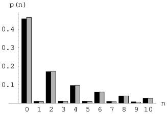
Figure 3.  : The photon distribution of a squeezed-thermal state as reconstructed by the ML estimation of the corresponding Wigner function (left histogram for the theoretical values, right histogram for the reconstructed values). Number of data samples $N=50000$, quantum efficiency $\eta=80\%$, number of thermal photons $n_{th}=0.1$, number of squeezing photons $n_{sq}=3$. The statistical error affects the third decimal digit, and it is not visible in the scale of the plot.

As a further development, we mention that the ML estimation of Gaussian Wigner functions also provides a technique to estimate the coupling constants of quadratic Hamiltonians of the form

$$\hat{H}=\alpha a+\alpha^{*}a^{\dagger}+\varphi a^{\dagger}a+\frac{1}{2}\xi a^{2}+\frac{1}{2}\xi^{*}a^{{\dagger}2}\;.$$ (19)

Hamiltonians like that in Eq. (19) describes the interaction of light modes in active optical medium characterized by a second order susceptibility tensor. Actually, the unitary evolution operator $\hat{U}=e^{-i\hat{H}t}$ preserves the Gaussian form of an input state with Gaussian Wigner function, and therefore one can use a Gaussian state to probe and characterize an optical device.

4.2 Absolute estimation of the quantum efficiency

The operation of a photodetector is, in principle, very simple: each photon ionizes an atom, and the resulting charge is amplified to produce a measurable pulse. In practice, however, available photodetectors are usually characterized by a quantum efficiency lower than unity, which means that only a fraction of the incoming photons lead to an electric pulse, and ultimately to a ”count”. We may distinguish two main classes of photodetectors. In the first we have detectors where the resulting current proportional to the incoming photon flux: in this case we have a linear photodetector. For example, this is the case of the high flux photodetectors used in homodyne detection. In the second class we have photodetectors operating at very low intensities, which resort to avalanche process in order to transform a single ionization event into a recordable pulse. This implies that one cannot discriminate between a single photon or many photons as the outcomes from such detectors are either a ”click”, corresponding to any number of photons, or ”nothing” which means that no photons have been revealed.

Conventional characterization of photodetectors resorts to prepare a reference state with known intensity, and then measuring which fraction of the signal is actually revealed. This unavoidably leads to rather poor performances when applied in the relevant regime of quantum signals. Detection losses, in facts, distorce the whole probability distribution of the quantity being measured, not only the average value. Moreover, we need the accurate knowledge of the quantum state of the reference signal. In the following, we apply the ML principle to the absolute estimation of the quantum efficiency of both linear and avalanche photodetectors. We show that, along with the reliable characterization of quantum signals, ML method is an effective and statistically efficient tool for characterizing the response of a photodetector to low-intensity and/or nonclassical states.

Let us first study the case of linear photodetectors. As a reference state we consider a squeezed-coherent state, measured by homodyne detection. The effect of non-unit quantum efficiency $\eta$ on the probability distribution of homodyne detection is twofold. We have both a rescaling of the mean value and a broadening of the distribution. For a squeezed state $|x_{0},r\rangle=D(x_{0})S(r)|0\rangle$ with the direction of squeezing parallel to the signal phase and to the phase of the homodyne detection (without loss of generality we set this phase equal to zero and $x_{0},r>0$ ) we have [19]

$$p_{\eta}(x)=\frac{1}{\sqrt{2\pi\Delta^{2}}}\exp\left[-\frac{(x-\eta x_{0})^{2}}{2\Delta^{2}}\right]\qquad\Delta^{2}=\frac{1}{4}\left(e^{-2r}+1-\eta\right)\;.$$ (20)

The total number of photons of the state is given by $n=x_{0}^{2}+\sinh^{2}r$, whereas the squeezing fraction is defined as $\gamma=\sinh^{2}r/n$. Apart from an irrelevant constant, the log-likelihood function can be written as

$$-L(\eta)=\log\Delta^{2}+\frac{1}{\Delta^{2}}\left(\overline{x^{2}}+\eta x_{0}^{2}-2\eta x_{0}\overline{x}\right)\;.$$ (21)

The resulting MLE is thus given by

$$\eta_{\sc ml}=1+e^{-2r}+\frac{1}{x_{0}^{2}}\left\{1-\sqrt{1+64x_{0}^{2}\left[\overline{x^{2}}+(1+e^{-2r})(x_{0}-2\overline{x}+x_{0}e^{-2r})x_{0}\right]}\right\}$$

A set of Monte Carlo simulated experiments confirmed that the Cramér-Rao bound is attained. The performances of the ML estimation can be compared to the ”naive” estimation based only on the measurement of the mean value, i.e. $\eta_{\sc av}=\overline{x}/x_{0}$. We expect the naive method to be less efficient, since the quantum efficiency not only rescales the mean value, but also spreads the variance of the homodyne distribution in Eq. (20). In Fig. 4, on the basis of a Monte Carlo simulated experiment, we compare the ML and the average-value methods in estimating the quantum efficiency through homodyne detection on a squeezed state. The advantages of ML method are apparent, especially for the estimation of low values of $\eta$.

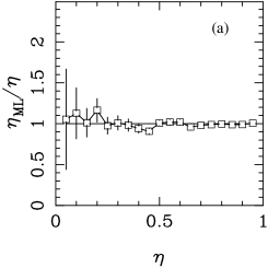
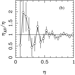
Figure 4.  : Quantum efficiency of linear photodetectors: ML estimation through homodyne detection on a squeezed state. The plots report the ratio between the estimated value of the quantum efficiency and the true value, as a function of the true value. On the left the results from maximum-likelihood method; on the right by the ”naive” average-value method. Homodyne sample: $2500$ data. Reference state: a squeezed state with mean number of photons $n=1$ and squeezing fraction $\gamma=99\%$ (nearly a squeezed vacuum).

Let us now consider avalanche photodetectors, which perform the ON/OFF measurement described by the two-value POM

$$\hat{\Pi}_{\sc off}=\sum_{p=0}^{\infty}(1-\eta)^{p}\>|p\rangle\langle p|\qquad\hat{\Pi}_{\sc on}={\bf I}-\hat{\Pi}_{\sc off}\;,$$ (22)

where ${\bf I}$ denotes the identity operator. With avalanche photodetectors we have only two possible outcomes: ”click” or ”no clicks” which we denote by ”1” and ”0” respectively. The log-likelihood function is given by

$$L(\eta)=(N-N_{c})\log P_{0}(\eta)+N_{c}\log[1-P_{0}(\eta)]\;,$$ (23)

where $P_{0}(\eta)=\hbox{Tr}[\hat{\varrho}\hat{\Pi}_{\sc off}]$ is the probability of having no clicks for the reference state described by the density matrix $\varrho$, $N$ is the total number of measurements, and $N_{c}$ is the number of events leading to a click. The maximum of $L(\eta)$, i.e. the MLE for the quantum efficiency, satisfies the equation

$$P_{0}(\eta_{\sc ml})=1-\frac{N_{c}}{N}\;,$$ (24)

whose solution, of course, depends on the choice of the reference state. The optimal choice would be using single-photon states as a reference. In this case, we have the trivial result $\eta_{\sc ml}=N_{c}/N$. However, single-photon state are not easy to prepare and generally one would like to test $\eta$ for coherent pulses $|\alpha\rangle$. In this case, we have $P_{0}(\eta)=\exp(-|\alpha|^{2}\eta)$ and

$$\eta_{\sc ml}=-\frac{1}{|\alpha|^{2}}\log\left(1-\frac{N_{c}}{N}\right)\;.$$ (25)

The Fisher information is given by

$$F=\left(\frac{\partial P_{0}}{\partial\eta}\right)^{2}\frac{1}{P_{0}}+\left(\frac{\partial P_{1}}{\partial\eta}\right)^{2}\frac{1}{P_{1}}=\frac{1}{P_{0}(1-P_{0})}\left(\frac{\partial P_{0}}{\partial\eta}\right)^{2}\;,$$ (26)

and therefore, for a weak coherent reference one has

$$F=\frac{\eta^{2}}{e^{\eta|\alpha|^{2}}-1}\simeq\frac{\eta}{|\alpha|^{2}}\qquad\sigma_{\eta} \simeq \frac{|\alpha|}{\sqrt{\eta N}}\>.$$ (27)

5 Summary and conclusions

In this paper we reviewed the application of the maximum likelihood principle to the reconstruction of the density matrix of a generic quantum system [9], as well as to the estimation of relevant parameters in quantum optics [10]. In all cases, the resulting reconstruction algorithm is statistically efficient, and provides the reliable estimation of the quantity of interest using much smaller data samples compared to conventional methods. In particular, the ML estimation of the density matrix allows one to incorporate the natural physical constraints we have on the quantum state, thus leading to a substantial reduction of statistical fluctuations. For quantum-optical parameters, the ML approach provides efficient estimation schemes based on feasible measurements like homodyne detection. The resulting procedures lead to substantial improvement over conventional methods and are of technological interest.

References

- 1. G. M. D’Ariano and H. P. Yuen, Phys. Rev. Lett. 76, 2832 (1996)
- 2. W. K. Wootters, W. H. Zurek, Nature, 299, 802 (1982); H. P. Yuen, Phys. Lett. A113, 405 (1986).
- 3. D. T. Smithey, M. Beck, M. G. Raymer, and A. Faridani, Phys. Rev. Lett. 70, 1244 (1993); G. Breitenbach, S. Schiller, and J. Mlynek, Nature 387, 471 (1997).
- 4. T. J. Dunn, I. A. Walmsley, and S. Mukamel, Phys. Rev. Lett. 74, 884 (1995).
- 5. D. Leibfried et al., Phys. Rev. Lett. 77, 4281 (1996).
- 6. Ch. Kurtsiefer, T. Pfau, and J. Mlynek, Nature 386, 150 (1997).
- 7. S. Massar and S. Popescu, Phys. Rev. Lett. 74, 1259 (1995); R. Derka, V. Bužek, and A. K. Ekert, Phys. Rev. Lett. 80, 1571 (1998).
- 8. G. M. D’Ariano, L. Maccone, M. G. A. Paris, Quorum of observables for universal quantum estimation, quant-ph/0006006.
- 9. K. Banaszek, G. M. D’Ariano, M. G. A. Paris, M. F. Sacchi, Phys. Rev. A 61, 10304(R) (2000).
- 10. G. M. D’Ariano, M. G. A. Paris, M. F. Sacchi, Parameter estimation in quantum optics, to appear in Phys. Rev. A (August 2000).
- 11. H. G. Tucker, Probability and mathematical statistics, Academic Press (1962).
- 12. H. Cramér, Mathematical methods of statistics, Princeton Press (1946).
- 13. In terms of -eigenvectors , one has as . The maximum likelihood condition gives . After multiplication by and summation over , one obtains .
- 14. W. H. Press, S. A. Teukolsky, W. T. Vetterling, B. P. Flannery: Numerical Recipes in Fortran: The Art of Scientific Computing (Cambridge University Press, Cambridge, 1992) Sec. 10.4
- 15. G. M. D’Ariano, U. Leonhardt, and H. Paul, Phys. Rev. A 52, R1801 (1995).
- 16. G. M. D’Ariano, P. Kumar, and M. F. Sacchi, Phys. Rev. A 59, 826 (1999).
- 17. G. M. D’Ariano, P. Kumar, and M. F. Sacchi, Phys. Rev. A 61, 013806 (2000).
- 18. H. P. Yuen, Phys. Rev. A 13, 2226 (1976).
- 19. U. Leonhardt and H. Paul, Phys. Rev. A 48, 4598 (1993)