Motional Casimir force

Abstract

We study the situation where two point like mirrors are placed in the vacuum state of a scalar field in a two-dimensional spacetime. Describing the scattering upon the mirrors by transmittivity and reflectivity functions obeying unitarity, causality and high frequency transparency conditions, we compute the fluctuations of the Casimir forces exerted upon the two motionless mirrors. We use the linear response theory to derive the motional forces exerted upon one mirror when it moves or when the other one moves. We show that these forces may be resonantly enhanced at the frequencies corresponding to the cavity modes. We interpret them as the mechanical consequence of generation of squeezed fields.

PACS: 03.65 - 42.50 - 12.20

Introduction

The vacuum fluctuations of the electromagnetic field manifest themselves through macroscopic Casimir forces [1, 2, 3]. These forces result from the radiation pressure exerted upon boundaries by the scattered fluctuations which depends upon the instantaneous and local value of the stress tensor. Consequently, they are fluctuating quantities [4]. More precisely, the forces exerted upon the two mirrors of a Fabry-Perot cavity have to be considered as random variables. In the present paper, we compute the associated correlation functions. For the sake of simplicity, we study the situation where two point like mirrors are placed in the vacuum state of a scalar field in a two-dimensional (2D) spacetime.

As illustrated by the Langevin theory of Brownian motion [5], any fluctuating force has a long term cumulative effect. This cumulative force can be derived from linear response theory [6]. The fluctuations of Casimir forces thus imply that mirrors moving in the vacuum must experience systematic forces. In a previous paper [7], we have computed such a motional force for a single mirror in the vacuum state (of a scalar field in a 2D spacetime). At the limit of perfect reflectivity, we found a dissipative force proportional to the third time derivative of the mirror’s position $q$

$$F\left(t\right)=\frac{\hbar q^{\prime\prime\prime}\left(t\right)}{6\pi c^{2}}$$ (1)

which corresponds to a linear susceptibility at the frequency $\omega$

$$\chi[\omega]=\frac{i\hbar\omega^{3}}{6\pi c^{2}}$$ (2)

(from now on, we use natural units where $c=1$; however, we keep $\hbar$ as a scale for vacuum fluctuations). This damping force for a single moving mirror is connected to the Casimir force (mean force between two mirrors at rest) since both result from a modification of the vacuum stress tensor [8]. Actually, expression (1a) identifies with the linear approximation of the force computed using the techniques of quantum field theory [9, 10, 11]. As required by Lorentz invariance of the vacuum state [12], the damping force vanishes for a motion with a uniform velocity. In the case of a uniform acceleration, the mirror is submitted to the same fluctuating field as if it were at rest in a thermal field [13] so that it experiences also a zero motional force.

In the present paper, we compute the explicit expressions of the forces exerted upon one mirror due either to its own motion (in presence of the second mirror) or to the motion of the other. These expressions, obtained from linear response theory, are valid in a first order expansion in the mirrors’ displacement without restriction on the motion’s frequency.

A problem in any calculation of vacuum induced effects is to dispose of the divergences associated with the infiniteness of the total vacuum energy. This problem can be solved by assuming that the boundaries are transparent at high frequencies. Using a scattering approach where the mirrors are described by transmittivity and reflectivity functions obeying unitarity, causality and high frequency transparency conditions, one obtains a regular expression for the mean force between two mirrors [3]. The same approach also provides directly a causal motional force in the single mirror problem whereas the non causal expression (1) is recovered as an asymptotic limit for a perfectly reflecting mirror [7].

In the present paper, we use this approach to study the motional forces in the two mirrors problem. First, we compute the correlation functions characterizing the fluctuating Casimir forces exerted upon the two motionless mirrors. Then, we use the linear response theory to derive the susceptibility functions associated with the motional forces. In order to obtain these functions, we use some analytic properties of the correlation functions which are analysed in Appendix A. We check that our results are consistent with already known limiting cases: the static Casimir force [3] (limit of a null frequency), the one mirror problem [7] (limit where one mirror is transparent) and the limit of perfect reflection [10].

The expressions obtained for perfectly reflecting mirrors correspond to a damping force analogous to equation (1) with two differences. First, the response is delayed because of the time of flight from one mirror to the other. Second, the motional modification of the vacuum fields is reflected back by the mirrors. The resulting interference between the different numbers of cavity roundtrips gives rise to a divergence of the susceptibility functions. For partially transmitting mirrors, these functions are regular and describe a resonant enhancement of the motional Casimir force, which may be large when the Fabry-Perot cavity has a high finesse [14]. A resonance approximation is used to evaluate the susceptibility functions in this case.

It is known that mirrors moving with a non uniform velocity squeeze the vacuum fields [15, 16]. This requires that energy and impulsion be exchanged between the mirrors and the fields. The motional Casimir forces thus appear as a mechanical consequence of this squeezing effect. In Appendix B, we discuss the motional modifications of the field scattering by the mirrors and we write an effective Hamiltonian describing the squeezing effect as well as the mechanical forces upon the mirrors.

Notations

Any function $f(t)$ defined in the time domain and its Fourier transform $f[\omega]$ are supposed to be related through

$$f(t)=\int\frac{{\rm d}\omega}{2\pi}f[\omega]e^{-i\omega t}$$ (3)

In the following, some functions of time will be expressed as integrals over two frequencies, with the notation

$$f(t)=\int\frac{{\rm d}\omega}{2\pi}\int\frac{{\rm d}\omega^{\prime}}{2\pi}e^{-i\omega t-i\omega^{\prime}t}f[\omega,\omega^{\prime}]$$ (4)

Comparing with (2a), one gets the equivalent expression

$$f[\omega]=\int\frac{{\rm d}\omega^{\prime}}{2\pi}f[\omega-\omega^{\prime},\omega^{\prime}]$$ (5)

In a 2D spacetime (time coordinate $t$, space coordinate $x$), a free scalar field is the sum of two counterpropagating components $\varphi(t-x)+\psi(t+x)$ which will be written as the two components of a column matrix

$\displaystyle\Phi_{x}(t)=\left(\begin{array}[]{c}\varphi(t-x)\\ \psi(t+x)\end{array}\right)$

The Fourier transform $\Phi_{x}[\omega]$ of the column $\Phi_{x}(t)$ is related to the standard annihilation and creation operators corresponding to the two propagation directions

$$\Phi_{x}[\omega]=\left(\begin{array}[]{c}\varphi[\omega]e^{i\omega x}\\ \psi[\omega]e^{-i\omega x}\end{array}\right)=e^{i\eta\omega x}\Phi[\omega]$$

$$\varphi[\omega]=\sqrt{\frac{\hbar}{2|\omega|}}\left(\theta(\omega)a_{\omega}+\theta(-\omega)a_{-\omega}^{\dagger}\right)\qquad\psi[\omega]=\sqrt{\frac{\hbar}{2|\omega|}}\left(\theta(\omega)b_{\omega}+\theta(-\omega)b_{-\omega}^{\dagger}\right)$$

where the abbreviated notation $\Phi$ stands for the values of $\Phi_{x}$ evaluated at $x=0$ and

$\displaystyle\eta=\left(\begin{array}[]{cc}1&0\\ 0&-1\end{array}\right)$

The energy and impulsion densities correspond to two counterpropagating energy fluxes

$\displaystyle e_{x}(t)=\varphi^{\prime}(t-x)^{2}+\psi^{\prime}(t+x)^{2}\qquad p_{x}(t)=\varphi^{\prime}(t-x)^{2}-\psi^{\prime}(t+x)^{2}$

They may be written as integrals over two frequencies (see eqs 2) with

$\displaystyle e_{x}[\omega,\omega^{\prime}]=i\omega i\omega^{\prime}\ \mathop{\rm Tr}\left[\Phi_{x}[\omega]\Phi_{x}[\omega^{\prime}]^{\rm T}\right]\qquad e_{x}[\omega,\omega^{\prime}]=i\omega i\omega^{\prime}\ \mathop{\rm Tr}\left[\eta\Phi_{x}[\omega]\Phi_{x}[\omega^{\prime}]^{\rm T}\right]$

$\mathop{\rm Tr}$ stands for the trace operation and $X^{\rm T}$ for the transposed of $X$. So, their mean values in a quantum state are functions of the covariance matrix

$\displaystyle\left\langle\Phi_{x}[\omega]\Phi_{x^{\prime}}[\omega^{\prime}]^{\rm T}\right\rangle=e^{i\eta\omega x}\left\langle\Phi[\omega]\Phi[\omega^{\prime}]^{\rm T}\right\rangle e^{i\eta\omega^{\prime}x^{\prime}}$

For a stationary state such as the vacuum, the covariance matrix depends only upon one frequency parameter

$$\left\langle\Phi[\omega]\Phi[\omega^{\prime}]^{\rm T}\right\rangle=2\pi\delta(\omega+\omega^{\prime})c[\omega]$$ (7)

It will be useful to write it in terms of the anticommutators which characterize the field states and of the commutators which do not depend upon the states

$$c[\omega]=c_{+}[\omega]+c_{-}[\omega]$$ ()

$$c_{+}[\omega] = \frac{c[\omega]+c[-\omega]^{\rm T}}{2}=c_{+}[-\omega]^{\rm T}\qquad c_{-}[\omega]=\frac{c[\omega]-c[-\omega]^{\rm T}}{2}=\frac{I\hbar}{4\omega}$$ (8)

$I$ is the unit matrix. The vacuum state corresponds to

$$c[\omega]=I\theta(\omega)\frac{\hbar}{2\omega}\qquad c_{+}[\omega]=I\varepsilon(\omega)\frac{\hbar}{4\omega}\qquad\varepsilon(\omega)=\theta(\omega)-\theta(-\omega)$$ (9)

Scattering upon motionless mirrors

The scattering of the field upon a partially transmitting mirror at rest at $q$ is described by

$$\Phi_{\rm out}[\omega]=e^{-i\eta\omega q}S[\omega]e^{i\eta\omega q}\Phi_{\rm in}[\omega]\qquad S[\omega]=\left(\begin{array}[]{cc}s[\omega]&r[\omega]\\ r[\omega]&s[\omega]\end{array}\right)$$ (9)

The $S-$matrix is supposed to be real in the temporal domain, causal and unitary

$$S[-\omega]=S[\omega]^{*}$$ ()

$$S[\omega]{\rm\ is\ analytic\ (and\ regular)\ for\ }\mathop{\rm Im}\omega>0$$ ()

$$S[\omega]S[\omega]^{\dagger}=1$$ ()

Finally, the mirror is supposed to be transparent at high frequencies

$$S[\omega]\rightarrow I{\rm\quad for\ }\omega\rightarrow\infty$$ (10)

This assumption will allow us to regularize the ultraviolet divergences associated with the infiniteness of the vacuum energy [3]. A mirror perfectly reflecting ($s=0$ and $r=-1$) at all frequencies does not obey this condition and it will be better to consider the perfect mirror as the limit of a model obeying the transparency condition (for example a mirror perfectly reflecting at frequencies below a reflection cutoff).

We study now the situation where two mirrors are placed at rest in the vacuum at positions $q_{1}$ and $q_{2}$ (see Figure 1).

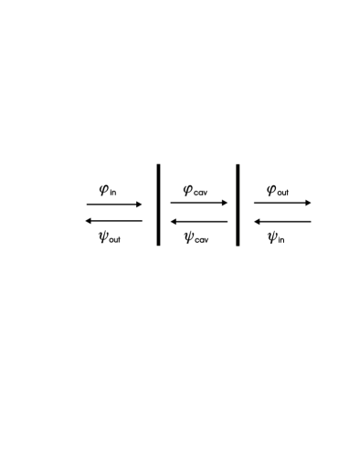
FIG. 1.: Two mirrors scatter the two counterpropagating fields. The subscripts ‘in’, ‘out’ and ‘cav’ refer respectively to the input, output and intracavity fields.

As the final results will depend only on the distance $q=q_{2}-q_{1}$ between the two mirrors, we consider from now on

$$q_{2}=\frac{q}{2}\qquad q_{1}=-\frac{q}{2}$$ (11)

The scattering of the field by the mirrors (see Figure 1) is described by two scattering matrices given by equations (5)

$$\left(\begin{array}[]{c}\varphi_{\rm cav}[\omega]\\ \psi_{\rm out}[\omega]\end{array}\right) = \left(\begin{array}[]{cc}s_{1}[\omega]&r_{1}[\omega]e^{i\omega q}\\ r_{1}[\omega]e^{-i\omega q}&s_{1}[\omega]\end{array}\right)\left(\begin{array}[]{c}\varphi_{\rm in}[\omega]\\ \psi_{\rm cav}[\omega]\end{array}\right)$$

$$\left(\begin{array}[]{c}\varphi_{\rm out}[\omega]\\ \psi_{\rm cav}[\omega]\end{array}\right) = \left(\begin{array}[]{cc}s_{2}[\omega]&r_{2}[\omega]e^{-i\omega q}\\ r_{2}[\omega]e^{i\omega q}&s_{2}[\omega]\end{array}\right)\left(\begin{array}[]{c}\varphi_{\rm cav}[\omega]\\ \psi_{\rm in}[\omega]\end{array}\right)$$

As usual in the computation of a Fabry Perot cavity, one can solve these equations to express the outcoming and the intracavity fields in terms of the input ones

$\displaystyle\Phi_{\rm out}[\omega]=S[\omega]\Phi_{\rm in}[\omega]\qquad\Phi_{\rm cav}[\omega]=R[\omega]\Phi_{\rm in}[\omega]$

The global scattering matrix $S[\omega]$ and the resonance matrix $R[\omega]$ are given by (all the reflectivities and transmittivities are evaluated at frequency $\omega$)

$$S[\omega]=\frac{1}{d[\omega]}\left(\begin{array}[]{cc}s_{1}s_{2}&r_{2}e^{-i\omega q}+d_{2}r_{1}e^{i\omega q}\\ r_{1}e^{-i\omega q}+d_{1}r_{2}e^{i\omega q}&s_{1}s_{2}\end{array}\right)$$ ()

$$R[\omega]=\frac{1}{d[\omega]}\left(\begin{array}[]{cc}s_{1}&s_{2}r_{1}e^{i\omega q}\\ s_{1}r_{2}e^{i\omega q}&s_{2}\end{array}\right)$$ ()

$$d_{1}[\omega]=s_{1}[\omega]^{2}-r_{1}[\omega]^{2}\qquad d_{2}[\omega]=s_{2}[\omega]^{2}-r_{2}[\omega]^{2}$$ (18)

$$d[\omega]=1-r[\omega]e^{2i\omega q}\qquad r[\omega]=r_{1}[\omega]r_{2}[\omega]$$ (19)

One checks from conditions (6) that the matrices $S$ and $R$ are real in the time domain, that they are retarded response functions, that the matrix $S$ is unitary and that the Fabry-Perot is transparent at the high frequency limit

$$S[-\omega]=S[\omega]^{*}\qquad R[-\omega]=R[\omega]^{*}$$ ()

$$S[\omega]{\rm\ and\ }R[\omega]{\rm\ are\ analytic\ (and\ regular)\ for\ }\mathop{\rm Im}\omega>0$$ ()

$$S[\omega]S[\omega]^{\dagger}=1$$ ()

$$S[\omega]\rightarrow I{\rm\quad}R[\omega]\rightarrow{\rm I\quad for\ }\omega\rightarrow\infty$$ ()

Casimir force between two motionless mirrors

As usual in a local formulation of the Casimir effect [17], the forces $F_{1}(t)$ and $F_{2}(t)$ acting upon the two mirrors can be deduced from the stress tensor evaluated at both sides of the mirrors

$$F_{1}(t) = \varphi_{\rm in}^{\prime}(t-q_{1})^{2}-\varphi_{\rm cav}^{\prime}(t-q_{1})^{2}+\psi_{\rm out}^{\prime}(t+q_{1})^{2}-\psi_{\rm cav}^{\prime}(t+q_{1})^{2}$$

$$F_{2}(t) = \varphi_{\rm cav}^{\prime}(t-q_{2})^{2}-\varphi_{\rm out}^{\prime}(t-q_{2})^{2}+\psi_{\rm cav}^{\prime}(t+q_{2})^{2}-\psi_{\rm in}^{\prime}(t+q_{2})^{2}$$

The forces are quadratic forms of the vacuum fields as the energy or impulsion densities, so that they can be expressed as integrals (2) over two frequencies with (using equation 7)

$$F_{1}[\omega,\omega^{\prime}] = \exp\left(-\frac{i}{2}(\omega+\omega^{\prime})q\right)i\omega i\omega^{\prime}\left(\varphi_{\rm in}[\omega]\varphi_{\rm in}[\omega^{\prime}]-\varphi_{\rm cav}[\omega]\varphi_{\rm cav}[\omega^{\prime}]\right)$$

$$+\exp\left(\frac{i}{2}(\omega+\omega^{\prime})q\right)i\omega i\omega^{\prime}\left(\psi_{\rm out}[\omega]\psi_{\rm out}[\omega^{\prime}]-\psi_{\rm cav}[\omega]\psi_{\rm cav}[\omega^{\prime}]\right)$$

$$F_{2}[\omega,\omega^{\prime}] = \exp\left(-\frac{i}{2}(\omega+\omega^{\prime})q\right)i\omega i\omega^{\prime}\left(\psi_{\rm cav}[\omega]\psi_{\rm cav}[\omega^{\prime}]-\psi_{\rm in}[\omega]\psi_{\rm in}[\omega^{\prime}]\right)$$

$$+\exp\left(\frac{i}{2}(\omega+\omega^{\prime})q\right)i\omega i\omega^{\prime}\left(\varphi_{\rm cav}[\omega]\varphi_{\rm cav}[\omega^{\prime}]-\varphi_{\rm out}[\omega]\varphi_{\rm out}[\omega^{\prime}]\right)$$

Noting that the matrices

$\displaystyle P_{\pm}=\frac{1\pm\eta}{2}$

are the projectors onto the counterpropagating components $\varphi$ and $\psi$ and using the expressions of the output and cavity fields in terms of the input ones, one obtains

$$F_{i}[\omega,\omega^{\prime}]=i\omega i\omega^{\prime}\ \mathop{\rm Tr}\left[{\cal F}_{i}[\omega,\omega^{\prime}]\Phi_{x}[\omega]\Phi_{x}[\omega^{\prime}]^{\rm T}\right]$$ (20)

with

$${\cal F}_{i}[\omega,\omega^{\prime}] = \varepsilon_{i}\exp\left(-\frac{i}{2}(\omega+\omega^{\prime})q\right)\left(P_{\varepsilon_{i}}-R[\omega^{\prime}]^{\rm T}P_{\varepsilon_{i}}R[\omega]\right)$$ (21)

$$+\varepsilon_{i}\exp\left(\frac{i}{2}(\omega+\omega^{\prime})q\right)\left(S[\omega^{\prime}]^{\rm T}P_{-\varepsilon_{i}}S[\omega]-R[\omega^{\prime}]^{\rm T}P_{-\varepsilon_{i}}R[\omega]\right)$$

$$\varepsilon_{1} = 1\qquad\varepsilon_{2}=-1$$ (22)

The two matrices ${\cal F}_{i}$ obey the following properties

$${\cal F}_{i}[\omega,\omega^{\prime}]^{\rm T}={\cal F}_{i}[\omega^{\prime},\omega]\qquad{\cal F}[\omega,\omega^{\prime}]^{\dagger}={\cal F}[-\omega^{\prime},-\omega]$$ (23)

When evaluating the mean forces in the vacuum, one obtains from equations (3,4)

$\displaystyle\left\langle F_{i}[\omega,\omega^{\prime}]\right\rangle=\theta(\omega)\frac{\hbar\omega}{2}2\pi\delta(\omega+\omega^{\prime})\ \mathop{\rm Tr}{\cal F}_{i}[\omega,-\omega]$

Using the unitarity of the $S-$matrix and the following expression of $RR^{\dagger}$

$$R[\omega]R[\omega]^{\dagger}=I+Q[\omega]+Q[\omega]^{\dagger}$$ ()

$$Q[\omega]=\frac{1}{d[\omega]}\left(\begin{array}[]{cc}r_{1}r_{2}e^{2i\omega q}&r_{1}e^{i\omega q}\\ r_{2}e^{i\omega q}&r_{1}r_{2}e^{2i\omega q}\end{array}\right)$$ ()

one shows that

$\displaystyle\mathop{\rm Tr}{\cal F}_{i}[\omega,-\omega]=\varepsilon_{i}\mathop{\rm Tr}\left(I-R[\omega]R[\omega]^{\dagger}\right)=-\varepsilon_{i}\mathop{\rm Tr}\left(Q[\omega]+Q[\omega]^{\dagger}\right)$

This leads to the known expression for the Casimir force between two partially transmitting mirrors [3]

$$\left\langle F_{i}(t)\right\rangle=-\varepsilon_{i}\int_{0}^{\infty}\frac{{\rm d}\omega}{2\pi}\hbar\omega\left(\frac{r[\omega]e^{2i\omega q}}{d[\omega]}+\frac{r[\omega]^{*}e^{-2i\omega q}}{d[\omega]^{*}}\right)$$ (25)

Force fluctuations

We now compute the correlation functions characterizing the fluctuations of the forces $F_{1}$ and $F_{2}$ acting upon the two mirrors

$\displaystyle C_{ij}(t)=\left\langle F_{i}(t)F_{j}(0)\right\rangle-\left\langle F_{i}\right\rangle\left\langle F_{j}\right\rangle$

Inserting the expressions (11) of the forces in terms of the field operators, it appears that the correlation functions $C_{ij}$ are related to fourth order moments or second order moments of annihilation or creation operators. With the help of Wick’s rules, the fourth order moments may be deduced from the second order ones. In simple words, the vacuum fields may be considered as stationary gaussian random variables and higher order statistical quantities can be deduced from the covariance matrix.

Using this method, simple algebraic manipulations lead to an expression of the functions $C_{ij}$ as integrals over two frequencies (see equations 2) with

$$C_{ij}[\omega,\omega^{\prime}]=2\omega^{2}\omega^{\prime\ 2}\ \mathop{\rm Tr}\left[{\cal F}_{i}[\omega,\omega^{\prime}]c_{\rm in}[\omega]{\cal F}_{j}[\omega,\omega^{\prime}]^{\dagger}c_{\rm in}[\omega^{\prime}]^{\rm T}\right]$$ (26)

This becomes for the vacuum state (see equation 4)

$$C_{ij}[\omega,\omega^{\prime}] = \frac{\hbar^{2}}{2}\theta(\omega)\theta(\omega^{\prime})\omega\omega^{\prime}\gamma_{ij}[\omega,\omega^{\prime}]$$ (27)

$$\gamma_{ij}[\omega,\omega^{\prime}] = \mathop{\rm Tr}\left[{\cal F}_{i}[\omega,\omega^{\prime}]{\cal F}_{j}[\omega,\omega^{\prime}]^{\dagger}\right]$$ ()

In other words, the noise spectra associated with the fluctuations of the Casimir forces may be written

$$C_{ij}[\omega]=\frac{\hbar^{2}}{2}\theta(\omega)\int_{0}^{\omega}\frac{{\rm d}\omega^{\prime}}{2\pi}\omega^{\prime}(\omega-\omega^{\prime})\gamma_{ij}[\omega^{\prime},\omega-\omega^{\prime}]$$ (28)

From properties (12), the coefficients $\gamma_{ij}$ obey

$\displaystyle\gamma_{ij}[\omega,\omega^{\prime}]=\gamma_{ij}[\omega^{\prime},\omega]=\gamma_{ji}[\omega,\omega^{\prime}]^{*}=\gamma_{ji}[-\omega,-\omega^{\prime}]$

Equations (16-17) give the correlation functions which characterize the fluctuations of the Casimir forces exerted upon the two mirrors. The explicit evaluation of the coefficients $\gamma_{ij}$ in terms of the scattering coefficients is given in the Appendix A (see equations 27 and 21).

Motional Casimir forces

We study now the motional Casimir forces. These forces could be obtained by analysing the modification of the stress tensor associated with the mirror’s motion [8]. At first order in the mirrors’ displacements, they can also be derived from the fluctuations computed for motionless mirrors by using the linear response theory [6]. We have used both methods and checked that they provide the same results, as it is the case in the single mirror problem [7]. Here, we present the linear response technique. The main steps of the other method are given in Appendix B.

The classical motion of the mirrors corresponds to an effective perturbation of the Hamiltonian

$$\delta H(t)=-\sum_{j}F_{j}(t)\delta q_{j}(t)$$ (29)

where $F_{j}$ are the force operators exerted upon the two mirrors. The linear response theory provides the mean motional forces associated with this perturbation in terms of susceptibility functions $\chi_{ij}$

$$\left\langle\delta F_{i}(t)\right\rangle=\sum_{j}{\int}{\rm d}\tau\ \chi_{ij}(\tau)\delta q_{j}(t-\tau)$$ (30)

The susceptibility functions $\chi_{ij}$ may be deduced from the correlation functions since they are the retarded parts of the mean values of the force commutators $\xi_{ij}$

$$\chi_{ij}(t) = 2i\theta(t)\xi_{ij}(t)$$ ()

$$\xi_{ij}(t) = \frac{\left[F_{i}(t),F_{j}(0)\right]}{2\hbar}=\frac{C_{ij}(t)-C_{ji}(-t)}{2\hbar}$$ ()

The motional forces will be conveniently characterized by the susceptibility functions written in the frequency domain (compare with equations 1)

$$\left\langle\delta F_{i}[\omega]\right\rangle=\sum_{j}\chi_{ij}[\omega]\delta q_{j}[\omega]$$ (31)

In a first step, we compute the force commutators from the correlation functions

$\displaystyle\xi_{ij}[\omega,\omega^{\prime}]=\frac{C_{ij}[\omega,\omega^{\prime}]-C_{ji}[-\omega^{\prime},-\omega]}{2\hbar}$

Using the properties (12) and writing the covariances (15) in terms of anticommutators and commutators (see equations 3), one shows that

$\displaystyle\xi_{ij}[\omega,\omega^{\prime}]=\frac{\omega\omega^{\prime}}{2}\mathop{\rm Tr}\left[{\cal F}_{j}[\omega,\omega^{\prime}]^{\dagger}{\cal F}_{i}[\omega,\omega^{\prime}]\omega c_{+,{\rm in}}[\omega]+{\cal F}_{j}[\omega^{\prime},\omega]^{\dagger}{\cal F}_{i}[\omega^{\prime},\omega]\omega^{\prime}c_{+,{\rm in}}[\omega^{\prime}]\right]$

In the vacuum state, this becomes (see equations 4 and 16)

$\displaystyle\xi_{ij}[\omega,\omega^{\prime}]=\frac{\hbar\omega\omega^{\prime}}{8}\left(\varepsilon(\omega)+\varepsilon(\omega^{\prime})\right)\gamma_{ij}[\omega,\omega^{\prime}]$

Writing the Fourier transform of the force commutator as

$\displaystyle\xi_{ij}[\omega]=\frac{\hbar}{4}\int_{0}^{\omega}\frac{{\rm d}\omega^{\prime}}{2\pi}\omega^{\prime}(\omega-\omega^{\prime})\gamma_{ij}[\omega^{\prime},\omega-\omega^{\prime}]$

one obtains the simple following relation with the noise spectrum (17)

$\displaystyle C_{ij}[\omega]=2\hbar\theta(\omega)\xi_{ij}[\omega]$

The noise spectrum $C_{ij}$ contains only positive frequency components, as expected for the zero temperature state. This corresponds to the fact that the vacuum fluctuations can damp the mirrors’ motion but cannot excite it [18].

In a second step, we deduce the susceptibility functions as the retarded part of the force commutators. This derivation relies upon the analytic properties of the correlation functions and requires a detailed inspection of the expression of the coefficients $\gamma_{ij}[\omega,\omega^{\prime}]$ in terms of the scattering coefficients. This analysis, presented in Appendix A, shows that $\xi_{ij}[\omega]$ is a sum of terms which are either retarded or advanced functions of $\omega$. The susceptibility functions $\chi_{ij}[\omega]$ are obtained by retaining only the retarded terms (see equations 19). One gets them as integrals over two frequencies with

$$\chi_{ij}[\omega,\omega^{\prime}]=\frac{i\hbar\omega\omega^{\prime}}{4}\left(\varepsilon(\omega)\gamma_{ij}^{R}[\omega,\omega^{\prime}]+\varepsilon(\omega^{\prime})\gamma_{ij}^{R}[\omega^{\prime},\omega]\right)$$ (32)

where the coefficients $\gamma_{ij}^{R}$ are the retarded parts of the coefficients $\gamma_{ij}$ considered as an analytic function of its second frequency parameter

$$\gamma_{11}^{R}[\omega,\omega^{\prime}] = 2\frac{\alpha_{1}[\omega,\omega^{\prime}]}{d[\omega]d[\omega^{\prime}]}+\alpha_{1}[\omega,\omega^{\prime}]\beta_{1}[\omega,\omega^{\prime}]r_{2}[\omega]\frac{e^{2i\omega q}}{d[\omega]}r_{2}[\omega^{\prime}]\frac{e^{2i\omega^{\prime}q}}{d[\omega^{\prime}]}$$ ()

$$+r_{1}[\omega^{\prime}]d_{1}[\omega]r_{2}[\omega]\frac{e^{2i\omega q}}{d[\omega]}+r_{1}[\omega]d_{1}[\omega^{\prime}]r_{2}[\omega^{\prime}]\frac{e^{2i\omega^{\prime}q}}{d[\omega^{\prime}]}$$

$$+\left(r_{1}[\omega]^{*}+r_{1}[\omega^{\prime}]\right)\left(r_{2}[\omega]^{*}e^{-2i\omega q}+r_{2}[\omega^{\prime}]e^{2i\omega^{\prime}q}\right)\frac{1}{d[\omega]d[\omega^{\prime}]}$$

$$+2-\frac{1}{d[\omega]}-\frac{1}{d[\omega^{\prime}]}$$

$$\gamma_{21}^{R}[\omega,\omega^{\prime}] = -\alpha_{1}[\omega,\omega^{\prime}]\alpha_{2}[\omega,\omega^{\prime}]\frac{e^{i\omega q}}{d[\omega]}\frac{e^{i\omega^{\prime}q}}{d[\omega^{\prime}]}-\left(r_{1}[\omega^{\prime}]+r_{1}[\omega]^{*}\right)\left(r_{2}[\omega^{\prime}]+r_{2}[\omega]^{*}\right)\frac{e^{-i\omega q}}{d[\omega]^{*}}\frac{e^{i\omega^{\prime}q}}{d[\omega^{\prime}]}$$ ()

$$\alpha_{i}[\omega,\omega^{\prime}] = 1-s_{i}[\omega]s_{i}[\omega^{\prime}]+r_{i}[\omega]r_{i}[\omega^{\prime}]$$ ()

$$\beta_{i}[\omega,\omega^{\prime}] = 1-s_{i}[\omega]s_{i}[\omega^{\prime}]-r_{i}[\omega]r_{i}[\omega^{\prime}]$$ ()

$\gamma_{22}^{R}$ and $\gamma_{12}^{R}$ are obtained by exchanging the roles of the two mirrors. It has to be noted that the coefficients $\gamma_{ij}^{R}$ are not symmetrical in the exchange of $\omega$ and $\omega^{\prime}$ so that the function $\chi_{ij}[\omega]$ is not an integral restricted to the interval $[0,\omega]$, in contrast to the functions $C_{ij}[\omega]$ (see equation 17) or $\xi_{ij}[\omega]$.

Equations (20-21) constitute the main results of this paper. They provide the expressions of the motional Casimir forces (see equations 19 and 2) for two partially reflecting mirrors in a linear approximation in the mirrors’ displacements.

Consistency with known results

Here, we check that the susceptivity functions (20) are consistent with already known results. This can be done in three limiting cases.

First, considering that the second mirror is transparent at all frequencies ($r_{2}=0$; $s_{2}=1$), one obtains

$$\chi_{11}[\omega,\omega^{\prime}]=\frac{i\hbar\omega\omega^{\prime}}{2}\left(\varepsilon(\omega)+\varepsilon(\omega^{\prime})\right)\alpha_{1}[\omega,\omega^{\prime}]$$ (36)

and one recovers the known susceptibility for a single partially transmitting mirror moving in the vacuum [7]

$$\chi_{11}[\omega]=i\hbar\int_{0}^{\omega}\frac{{\rm d}\omega^{\prime}}{2\pi}\omega^{\prime}(\omega-\omega^{\prime})\alpha_{1}[\omega^{\prime},\omega-\omega^{\prime}]$$ (37)

Then, the quasistatic susceptibilities can be computed from equation (20)

$$\chi_{ij}[0] = \int\frac{{\rm d}\omega}{2\pi}\chi_{ij}[\omega,-\omega]$$

$$\chi_{ij}[\omega,-\omega] = \frac{i\hbar\omega^{2}}{4}\varepsilon(\omega)\left(\gamma_{ij}^{R}[-\omega,\omega]-\gamma_{ij}^{R}[\omega,-\omega]\right)$$

Using equations (21), one checks that they are consistent with the mean Casimir force (14) between two motionless mirrors

$\displaystyle\chi_{ij}[0]=2i\hbar\varepsilon_{i}\varepsilon_{j}\int_{0}^{\infty}\frac{{\rm d}\omega}{2\pi}\omega^{2}\left(\frac{r[\omega]e^{2i\omega q}}{d[\omega]^{2}}-\frac{r[\omega]^{*}e^{-2i\omega q}}{d[\omega]^{*\ 2}}\right)=\partial_{q_{j}}\left\langle F_{i}\right\rangle$

Finally, one can consider the limiting case of perfectly reflecting mirrors ($r_{1}=r_{2}=-1$; $s_{1}=s_{2}=0$) where the expressions (21) may be simplified to

$$\gamma_{11}^{R}[\omega,\omega^{\prime}] = 2\left(\frac{2}{d[\omega^{\prime}]}-1\right)\left(\frac{1}{d[\omega]}+\frac{1}{d[-\omega]}-1\right)+2$$

$$\gamma_{21}^{R}[\omega,\omega^{\prime}] = -4\frac{e^{i\omega^{\prime}q}}{d[\omega^{\prime}]}\left(\frac{e^{i\omega q}}{d[\omega]}+\frac{e^{-i\omega q}}{d[-\omega]}\right)$$

Simple calculations then lead to the following expression of the motional force in the time domain

$$\left\langle\delta F_{1}(t)\right\rangle = \frac{\hbar}{6\pi}\left(\delta q_{1}^{\prime\prime\prime}(t)+\delta q_{1}^{\prime\prime\prime}(t-2q)+\delta q_{1}^{\prime\prime\prime}(t-4q)+\ldots-\delta q_{2}^{\prime\prime\prime}(t-q)-\delta q_{2}^{\prime\prime\prime}(t-3q)-\ldots\right)$$ ()

$$+\frac{\hbar\pi}{6q^{2}}\left(\frac{1}{2}\delta q_{1}^{\prime}(t)+\delta q_{1}^{\prime}(t-2q)+\delta q_{1}^{\prime}(t-4q)+\ldots-\delta q_{2}^{\prime}(t-q)-\delta q_{2}^{\prime}(t-3q)-\ldots\right)$$

It can be checked that this is exactly the linear approximation [19] of the expression obtained for perfectly reflecting mirrors by Fulling and Davies [10]. The terms proportional to third time derivatives appear as generalizing the damping force (1) for a single perfectly reflecting mirror. Now, the force exerted upon one mirror depends not only on its own motion but also on the motion of the other one. The response is delayed due to the time of flight between the two mirrors: the motional modification of the stress tensor has to propagate from one mirror to the other in order to exert a force on it. Moreover, the modified stress tensor is reflected back by the two mirrors. The other terms, proportional to velocities, are not present in the one mirror problem because of the Lorentz invariance of the vacuum (see the discussion in the introduction). They are associated with the existence of a static Casimir force in the two mirrors problem.

Resonant enhancement of the motional Casimir force

The expression (23) leads to a divergence of the susceptibility functions when evaluated at the frequencies $\frac{k\pi}{q}$ with $k$ integer. Indeed, the contributions corresponding to different numbers of roundtrips give rise to a constructive interference at those frequencies. In other words, the Fabry-Perot can be considered as a mechanical resonator with resonance frequencies corresponding to the optical resonance frequencies.

For partially transmitting mirrors, the divergences due to perfect reflection will be regularized. In the last section of this paper, we evaluate the resonance enhancement at the limiting case of a large quality factor.

In this case, the reflection delays are much shorter than a roundtrip time and the reflectivity functions are smoother in the frequency domain than the Airy function describing the cavity modes. Replacing in (21) the denominators by geometrical series, we obtain each quantity $\gamma_{ij}^{R}$ as a sum of components evolving at different frequencies: this expansion is analogous to the one used in the computation of the static Casimir force at the large distance approximation [3]

$$\gamma_{11}^{R}[\omega,\omega^{\prime}] = 2\alpha_{1}[\omega,\omega^{\prime}]\sum_{l,m\geq 0}r[\omega]^{l}r[\omega^{\prime}]^{m}e^{2il\omega q+2im\omega^{\prime}q}$$

$$+\alpha_{1}[\omega,\omega^{\prime}]\beta_{1}[\omega,\omega^{\prime}]r_{2}[\omega]r_{2}[\omega^{\prime}]\sum_{l,m\geq 1}r[\omega]^{l-1}r[\omega^{\prime}]^{m-1}e^{2il\omega q+2im\omega^{\prime}q}$$

$$+\left(r_{1}[-\omega]+r_{1}[\omega^{\prime}]\right)r_{2}[-\omega]\sum_{l\geq 1,m\geq 0}r[-\omega]^{l-1}r[\omega^{\prime}]^{m}e^{-2il\omega q+2im\omega^{\prime}q}$$

$$+\left(r_{1}[-\omega]+r_{1}[\omega^{\prime}]\right)r_{2}[\omega^{\prime}]\sum_{l\geq 0,m\geq 1}r[-\omega]^{l}r[\omega^{\prime}]^{m-1}e^{-2il\omega q+2im\omega^{\prime}q}$$

$$+r_{1}[\omega^{\prime}]d_{1}[\omega]r_{2}[\omega]\sum_{l\geq 1}r[\omega]^{l-1}e^{2il\omega q}$$

$$+r_{1}[\omega]d_{1}[\omega^{\prime}]r_{2}[\omega^{\prime}]\sum_{m\geq 1}r[\omega^{\prime}]^{m-1}e^{2im\omega^{\prime}q}$$

$$-\sum_{l\geq 1}r[\omega]^{l}e^{2il\omega q}-\sum_{m\geq 1}r[\omega^{\prime}]^{m}e^{2im\omega^{\prime}q}$$

$$\gamma_{21}^{R}[\omega,\omega^{\prime}] = -\alpha_{1}[\omega,\omega^{\prime}]\alpha_{2}[\omega,\omega^{\prime}]\sum_{l,m\geq 0}r[\omega]^{l}r[\omega^{\prime}]^{m}e^{i\left(2l+1\right)\omega q+i\left(2m+1\right)\omega^{\prime}q}$$

$$-\left(r_{1}[\omega^{\prime}]+r_{1}[-\omega]\right)\left(r_{2}[\omega^{\prime}]+r_{2}[-\omega]\right)\sum_{l,m\geq 0}r[-\omega]^{l}r[\omega^{\prime}]^{m}e^{-i\left(2l+1\right)\omega q+i\left(2m+1\right)\omega^{\prime}q}$$

We will denote $\mu_{ij}^{(L,M)}$ the coefficients in this expansion

$\displaystyle\gamma_{ij}^{R}[\omega,\omega^{\prime}]=\sum_{L,M}\mu_{ij}^{(L,M)}[\omega,\omega^{\prime}]e^{iL\omega q+iM\omega^{\prime}q}$

The coefficients $\mu_{ij}^{(L,M)}$ depend only upon the reflectivity functions. Negative values of $M$ do not appear in the sum because $\mu_{ij}^{(L,M)}[\omega,\omega^{\prime}]$ is a retarded function of $\omega^{\prime}$. Only even values of $L$ and $M$ appear for $i=j$ and odd ones for $i\neq j$.

Then, the susceptibility functions $\chi_{ij}[\omega]$ will be obtained through an integration (see equations 2)

$$\chi_{ij}[\omega] = \sum_{L,M}\chi_{ij}^{(L,M)}[\omega]$$ ()

$$\chi_{ij}^{(L,M)}[\omega] = {\int}\frac{{\rm d}\omega^{\prime}}{2\pi}\chi_{ij}^{(L,M)}[\omega^{\prime},\omega-\omega^{\prime}]$$ ()

$$\chi_{ij}^{(L,M)}[\omega,\omega^{\prime}] = \frac{i\hbar}{4}\omega\omega^{\prime}\left(\varepsilon(\omega)\mu_{ij}^{(L,M)}[\omega,\omega^{\prime}]e^{iL\omega q+iM\omega^{\prime}q}+\varepsilon(\omega^{\prime})\mu_{ij}^{(L,M)}[\omega^{\prime},\omega]e^{iL\omega^{\prime}q+iM\omega q}\right)$$ ()

It follows that the integrals $\chi_{ij}^{(L,M)}$ with $L\neq M$ will contain exponentials with a rapidly varying phase and can be considered as non resonant terms. At the limit of perfect reflection, they provide the terms proportional to the velocities in equations (23) while the resonant terms $\chi_{ij}^{(L,M)}$ with $L=M$ provide the terms proportional to the third time derivatives.

In order to obtain the behaviour of the susceptibility functions near a resonance at $\frac{k\pi}{q}$ with $k$ a large integer, we will retain only the terms $L=M$ (the first time derivatives have a small contribution to equation 23 compared to the third time derivatives in this case). In this resonance approximation, we obtain

$$\gamma_{11}^{R}[\omega,\omega^{\prime}]=\sum_{l\geq 0}\mu_{11}^{(2l,2l)}[\omega,\omega^{\prime}]e^{2il(\omega+\omega^{\prime})q}$$

$$\mu_{11}^{(2l,2l)}[\omega,\omega^{\prime}]=2\alpha_{1}[\omega,\omega^{\prime}]r[\omega]^{l}r[\omega^{\prime}]^{l}+\theta_{l\geq 1}\alpha_{1}[\omega,\omega^{\prime}]\beta_{1}[\omega,\omega^{\prime}]r_{2}[\omega]r_{2}[\omega^{\prime}]r[\omega]^{l-1}r[\omega^{\prime}]^{l-1}$$

$$\gamma_{21}^{R}[\omega,\omega^{\prime}]=\sum_{l\geq 0}\mu_{21}^{(2l+1,2l+1)}[\omega,\omega^{\prime}]e^{i(2l+1)(\omega+\omega^{\prime})q}$$

$$\mu_{21}^{(2l+1,2l+1)}[\omega,\omega^{\prime}]=-\alpha_{1[}\omega,\omega^{\prime}]\alpha_{2}[\omega,\omega^{\prime}]r[\omega]^{l}r[\omega^{\prime}]^{l}$$

$\theta_{l\geq 1}=0$ for $l=0$ and $\theta_{l\geq 1}=1$ for $l\geq 1$. As these expressions are symmetrical in the exchange of the two parameters $\omega$ and $\omega^{\prime}$ (this was not the case for the general expressions 21 of $\gamma_{ij}^{R}$), equations (24) lead to

$$\chi_{ij}[\omega] = \sum_{L}\chi_{ij}^{(L,L)}[\omega]$$

$$\chi_{ij}^{(L,L)}[\omega] = \frac{i\hbar}{2}e^{iL\omega q}{\int_{0}^{\omega}}\frac{{\rm d}\omega^{\prime}}{2\pi}\omega^{\prime}(\omega-\omega^{\prime})\mu_{ij}^{(L,L)}[\omega^{\prime},\omega-\omega^{\prime}]$$

The various terms $\chi_{ij}^{(L,L)}$ correspond to a motional force evaluated at a delay time close to a multiple of the time of flight $q$ between the two mirrors. For example, the term $\chi_{ij}^{(0,0)}$ describes the response of the force $F_{1}$ to the motion $q_{1}$ evaluated at times much shorter than the roundtrip time. As it could be expected, it does not depend upon the presence of the second mirror and is the same as if the mirror 1 were alone (compare $\mu_{11}^{(0,0)}[\omega,\omega^{\prime}]=2\alpha_{1}[\omega,\omega^{\prime}]$ with equation 22). The other contributions to $\chi_{11}$ correspond to the modification of the damping force due to the presence of the second mirror. They depend upon the reflectivities of the two mirrors and appear at time delays close to a multiple of the roundtrip time $2q$.

The terms $\chi_{21}^{(L,L)}$ describe the force exerted upon one mirror when the other one moves. They depend upon the reflectivity of both mirrors and appear at time delays close to an odd multiple of the time of flight $q$. The lowest order term has a simple form

$\displaystyle\mu_{21}^{(1,1)}[\omega,\omega^{\prime}]=-\alpha_{1}[\omega,\omega^{\prime}]\alpha_{2}[\omega,\omega^{\prime}]$

The moving mirror modifies the stress tensor of the vacuum field (modification described by the function $\alpha_{1}$). Then the radiation pressure experienced by the other mirror registers the modification of the stress tensor (detection efficiency described by the function $\alpha_{2}$).

In the limiting case of perfect reflection at all frequencies lower than $\omega$, one recovers the terms proportional to the third time derivatives in equations (23). The susceptibility functions diverge in this case but they are regular as soon as the mirrors have a small partial transmission. Indeed, the contributions corresponding to different numbers of roundtrips can be summed up to give in the resonance approximation

$$\gamma_{11}^{R}[\omega,\omega^{\prime}] = \frac{2\alpha_{1}[\omega,\omega^{\prime}]+\alpha_{1}[\omega,\omega^{\prime}]\beta_{1}[\omega,\omega^{\prime}]r_{2}[\omega]r_{2}[\omega^{\prime}]e^{2i(\omega+\omega^{\prime})q}}{D[\omega,\omega^{\prime}]}$$

$$\gamma_{21}^{R}[\omega,\omega^{\prime}] = -\frac{\alpha_{1}[\omega,\omega^{\prime}]\alpha_{2}[\omega,\omega^{\prime}]e^{i(\omega+\omega^{\prime})q}}{D[\omega,\omega^{\prime}]}$$

$$D[\omega,\omega^{\prime}] = 1-r[\omega]r[\omega^{\prime}]e^{2i(\omega+\omega^{\prime})q}$$

The denominator $D$ characterizes the resonances of the Fabry Perot cavity considered as a mechanical resonator.

Considering that the reflectivity coefficients may be approximated as constant functions from $0$ to $\omega$, the susceptibility functions are given by the simple expressions ($r=r_{1}r_{2}$)

$$\gamma_{11}^{R}[\omega,\omega^{\prime}]=\frac{4r_{1}^{2}}{1-r^{2}e^{2i(\omega+\omega^{\prime})q}}$$

$$\gamma_{21}^{R}[\omega,\omega^{\prime}]=-\frac{4r^{2}e^{i(\omega+\omega^{\prime})q}}{1-r^{2}e^{2i(\omega+\omega^{\prime})q}}$$

$$\chi_{11}[\omega]=\frac{i\hbar\omega^{3}}{6\pi}\frac{r_{1}^{2}}{1-r^{2}e^{2i\omega q}}$$

$$\chi_{21}[\omega]=-\frac{i\hbar\omega^{3}}{6\pi}\frac{r^{2}e^{i\omega q}}{1-r^{2}e^{2i\omega q}}$$

corresponding to a motional force

$\displaystyle\left\langle\delta F_{1}(t)\right\rangle=\frac{\hbar}{6\pi}\left(r_{1}^{2}\left(\delta q_{1}^{\prime\prime\prime}(t)+r^{2}\delta q_{1}^{\prime\prime\prime}(t-2q)+r^{4}\delta q_{1}^{\prime\prime\prime}(t-4q)+\ldots\right)-r^{2}\delta q_{2}^{\prime\prime\prime}(t-q)-r^{4}\delta q_{2}^{\prime\prime\prime}(t-3q)-\ldots\right)$

When compared with equation (23), one notes that the first time derivatives do not appear here because of the resonance approximation (the expression is valid only at high enough frequencies $\omega\gg\frac{\pi}{q}$). But the effect of imperfect reflection of the mirrors is now taken into account ($r_{1}^{2}$ and $r_{2}^{2}$ are the reflection coefficients of the two mirrors for energy densities) and the susceptibilities are regular functions of the frequency.

Conclusion

The motional Casimir force constitutes a new type of interaction between two mirrors. As the stationary Casimir effect, it is associated with a modification of the vacuum stress tensor due to the field scattering upon the mirrors. But it is resonantly enhanced at the resonance frequencies of the optical cavity $\frac{k\pi}{q}$. When compared with the case of a single mirror, the enhancement may reach the value $\frac{r_{1}^{2}}{1-r_{1}^{2}r_{2}^{2}}$. Consequently, the motional force might be very large [20] with the high finesse cavities such as those used in cavity QED [14].

Acknowledgements

We thank A. Heidmann for discussions.

A Analytic properties of the correlation functions

For the sake of clarity, we recall here the expressions of the susceptibility functions (see equations 2 and 19)

$$\chi_{ij}(t) = 2i\theta(t)\xi_{ij}(t)$$ ()

$$\xi_{ij}(t) = \int\frac{{\rm d}\omega}{2\pi}\int\frac{{\rm d}\omega^{\prime}}{2\pi}e^{-i\omega t-i\omega^{\prime}t}\xi_{ij}[\omega,\omega^{\prime}]$$ ()

$$\xi_{ij}[\omega,\omega^{\prime}] = \frac{\hbar\omega\omega^{\prime}}{8}\left(\varepsilon(\omega)+\varepsilon(\omega^{\prime})\right)\gamma_{ij}[\omega,\omega^{\prime}]$$ ()

Since the susceptibilities are related to the retarded part of the correlation functions, their derivation relies upon the analytic properties of the coefficients $\gamma_{ij}$. We show here how these properties can be inferred from the expressions of the coefficients $\gamma_{ij}$ in terms of the scattering coefficients, which are themselves analytic functions of the frequency (see equations 10). The coefficients $\gamma_{ij}$ are obtained from products of two matrices ${\cal F}_{i}$ (see equation 16) which are functions of the scattering and resonance matrices $S$ and $R$ (see equation 11b). Developping the corresponding expressions, one obtains rather lengthy expressions.

However, these expressions may be simplified by using the following properties. First the $S-$matrix is unitary ($S[\omega]S[\omega]^{\dagger}=I$) and the matrix $R[\omega]R[\omega]^{\dagger}$ may be written in terms of the retarded (analytic for $\mathop{\rm Im}\omega>0$) and advanced (analytic for $\mathop{\rm Im}\omega<0$) components $Q[\omega]$ and $Q[\omega]^{\dagger}$ (see equations 13). Then, it is also possible to reduce products $R[\omega]S[\omega]^{\dagger}$ and $S[\omega]R[\omega]^{\dagger}$ by noting that they determine the expression of the intracavity fields in terms of the output ones

$\displaystyle\Phi_{\rm cav}[\omega]=R[\omega]S[\omega]^{\dagger}\ \Phi_{\rm out}[\omega]$

Hence, $R[\omega]S[\omega]^{\dagger}$ is an advanced response function and its adjoint $S[\omega]R[\omega]^{\dagger}$ is a retarded one. Simple manipulations lead to

$$S[\omega]R[\omega]^{\dagger} = \overline{R}[\omega]\qquad R[\omega]S[\omega]^{\dagger}=\overline{R}[\omega]^{\dagger}$$ ()

$$\overline{R}[\omega] = \frac{1}{d[\omega]}\left(\begin{array}[]{cc}s_{2}&s_{2}r_{1}e^{i\omega q}\\ s_{1}r_{2}e^{i\omega q}&s_{1}\end{array}\right)$$ ()

Using these properties, the coefficients $\gamma_{ij}$ are written as sums of terms, each of them being easily recognized as either a retarded or an advanced function of the two frequency parameters $\omega$ and $\omega^{\prime}$

$$\gamma_{ij}[\omega,\omega^{\prime}] = \varepsilon_{i}\varepsilon_{j}\left(\mathop{\rm Tr}\left[P_{\varepsilon_{i}}P_{\varepsilon_{j}}+P_{-\varepsilon_{i}}P_{-\varepsilon_{j}}\right]\right.$$

$$-\mathop{\rm Tr}\left[P_{\varepsilon_{i}}R[\omega]P_{\varepsilon_{j}}R[\omega^{\prime}]^{\rm T}+P_{\varepsilon_{i}}R[\omega]^{\dagger}P_{\varepsilon_{j}}R[\omega^{\prime}]^{*}\right]$$

$$-\mathop{\rm Tr}\left[P_{-\varepsilon_{i}}\overline{R}[\omega]P_{-\varepsilon_{j}}\overline{R}[\omega^{\prime}]^{\rm T}+P_{-\varepsilon_{i}}\overline{R}[\omega]^{\dagger}P_{-\varepsilon_{j}}\overline{R}[\omega^{\prime}]^{*}\right]$$

$$+\mathop{\rm Tr}\left[P_{\varepsilon_{i}}\left(I+Q[\omega]+Q[\omega]^{\dagger}\right)P_{\varepsilon_{j}}\left(I+Q[\omega^{\prime}]^{\rm T}+Q[\omega^{\prime}]^{*}\right)\right]$$

$$+\mathop{\rm Tr}\left[P_{-\varepsilon_{i}}\left(I+Q[\omega]+Q[\omega]^{\dagger}\right)P_{-\varepsilon_{j}}\left(I+Q[\omega^{\prime}]^{\rm T}+Q[\omega^{\prime}]^{*}\right)\right]$$

$$+e^{i(\omega+\omega^{\prime})q}\mathop{\rm Tr}\left[P_{-\varepsilon_{i}}S[\omega]P_{\varepsilon_{j}}S[\omega^{\prime}]^{\rm T}\right]+e^{-i(\omega+\omega^{\prime})q}\mathop{\rm Tr}\left[P_{\varepsilon_{i}}S[\omega]^{\dagger}P_{-\varepsilon_{j}}S[\omega^{\prime}]^{*}\right]$$

$$-e^{i(\omega+\omega^{\prime})q}\mathop{\rm Tr}\left[P_{-\varepsilon_{i}}R[\omega]P_{\varepsilon_{j}}R[\omega^{\prime}]^{\rm T}+P_{-\varepsilon_{i}}\overline{R}[\omega]P_{\varepsilon_{j}}\overline{R}[\omega^{\prime}]^{\rm T}\right]$$

$$-e^{-i(\omega+\omega^{\prime})q}\mathop{\rm Tr}\left[P_{\varepsilon_{i}}R[\omega]^{\dagger}P_{-\varepsilon_{j}}R[\omega^{\prime}]^{*}+P_{\varepsilon_{i}}\overline{R}[\omega]^{\dagger}P_{-\varepsilon_{j}}\overline{R}[\omega^{\prime}]^{*}\right]$$

$$+e^{i(\omega+\omega^{\prime})q}\mathop{\rm Tr}\left[P_{-\varepsilon_{i}}\left(I+Q[\omega]+Q[\omega]^{\dagger}\right)P_{\varepsilon_{j}}\left(I+Q[\omega^{\prime}]^{\rm T}+Q[\omega^{\prime}]^{*}\right)\right]$$

$$+\left.e^{-i(\omega+\omega^{\prime})q}\mathop{\rm Tr}\left[P_{\varepsilon_{i}}\left(I+Q[\omega]+Q[\omega]^{\dagger}\right)P_{-\varepsilon_{j}}\left(I+Q[\omega^{\prime}]^{\rm T}+Q[\omega^{\prime}]^{*}\right)\right]\right)$$

Now, the susceptibility functions $\chi_{ij}$ are obtained by retaining the retarded terms and dropping the advanced ones in $\xi_{ij}$ (see equations 25). Consider first the contribution of a term which contains the factor $\varepsilon(\omega)$, which is still an analytic function of $\omega^{\prime}$ but not of $\omega$. Its integration over $\omega^{\prime}$ (see equations 25) provides a contribution to $\chi_{ij}(t)$ which is either retarded (vanishing for $t<0$) or advanced (vanishing for $t>0$). Some terms do not depend upon $\omega^{\prime}$ and their integration contributes for a half to retarded terms and for a half to advanced ones as can be verified explicitly on expressions (25). The terms containing the factor $\varepsilon(\omega^{\prime})$ are computed in the same manner by considering the integration over $\omega$.

One finally obtains $\chi_{ij}(t)$ as an integral over two frequencies (see equations 2) with

$\displaystyle\chi_{ij}[\omega,\omega^{\prime}]=\frac{i\hbar\omega\omega^{\prime}}{4}\left(\varepsilon(\omega)\gamma_{ij}^{R}[\omega,\omega^{\prime}]+\varepsilon(\omega^{\prime})\gamma_{ij}^{R}[\omega^{\prime},\omega]\right)$

where $\gamma_{ij}^{R}$ is the retarded part of $\gamma_{ij}$ considered as a function of its second frequency parameter, that is (assuming $q>0$)

$$\gamma_{ij}^{R}[\omega,\omega^{\prime}] = \varepsilon_{i}\varepsilon_{j}\left(\frac{1}{2}\mathop{\rm Tr}\left[P_{\varepsilon_{i}}P_{\varepsilon_{j}}+P_{-\varepsilon_{i}}P_{-\varepsilon_{j}}\right]\right.$$

$$-\mathop{\rm Tr}\left[P_{\varepsilon_{i}}R[\omega]P_{\varepsilon_{j}}R[\omega^{\prime}]^{\rm T}\right]-\mathop{\rm Tr}\left[P_{-\varepsilon_{i}}\overline{R}[\omega]P_{-\varepsilon_{j}}\overline{R}[\omega^{\prime}]^{\rm T}\right]$$

$$+\mathop{\rm Tr}\left[P_{\varepsilon_{i}}\left(I+Q[\omega]+Q[\omega]^{\dagger}\right)P_{\varepsilon_{j}}\left(\frac{I}{2}+Q[\omega^{\prime}]^{\rm T}\right)\right]$$

$$+\mathop{\rm Tr}\left[P_{-\varepsilon_{i}}\left(I+Q[\omega]+Q[\omega]^{\dagger}\right)P_{-\varepsilon_{j}}\left(\frac{I}{2}+Q[\omega^{\prime}]^{\rm T}\right)\right]$$

$$+e^{i(\omega+\omega^{\prime})q}\mathop{\rm Tr}\left[P_{-\varepsilon_{i}}S[\omega]P_{\varepsilon_{j}}S[\omega^{\prime}]^{\rm T}\right]$$

$$-e^{i(\omega+\omega^{\prime})q}\mathop{\rm Tr}\left[P_{-\varepsilon_{i}}R[\omega]P_{\varepsilon_{j}}R[\omega^{\prime}]^{\rm T}+P_{-\varepsilon_{i}}\overline{R}[\omega]P_{\varepsilon_{j}}\overline{R}[\omega^{\prime}]^{\rm T}\right]$$

$$+e^{i(\omega+\omega^{\prime})q}\mathop{\rm Tr}\left[P_{-\varepsilon_{i}}\left(I+Q[\omega]+Q[\omega]^{\dagger}\right)P_{\varepsilon_{j}}\left(I+Q[\omega^{\prime}]^{\rm T}\right)\right]$$

$$+\left.e^{-i(\omega+\omega^{\prime})q}\mathop{\rm Tr}\left[P_{\varepsilon_{i}}\left(I+Q[\omega]+Q[\omega]^{\dagger}\right)P_{-\varepsilon_{j}}Q[\omega^{\prime}]^{\rm T}\right]\right)$$

Using the expressions (8), (9), (13) and (26) of the matrices $S$, $R$, $Q$ and $\overline{R}$ in terms of the scattering coefficients describing the two mirrors, algebraic manipulations lead to the expressions (21) of the coefficients $\gamma_{ij}^{R}$.

As discussed previously, the coefficients $\gamma_{ij}$ contain terms corresponding to retarded contributions and which appear also in the coefficients $\gamma_{ij}^{R}$. The other terms correspond to advanced contributions and have been dropped. A comparison between the two types of terms shows that the coefficients $\gamma_{ij}$ can be deduced in a simple manner from the coefficients $\gamma_{ij}^{R}$

$$\gamma_{ij}[\omega,\omega^{\prime}]=\gamma_{ij}^{R}[\omega,\omega^{\prime}]+\gamma_{ji}^{R}[\omega,\omega^{\prime}]^{*}$$ (A3)

This relation between the correlation function and the susceptibility function may be considered as the expression of the fluctuation dissipation theorem [6] for the present problem. With the help of expressions (21), it provides the explicit expressions of the coefficients $\gamma_{ij}$ in terms of the scattering coefficients.

B Connection with squeezing

In the one mirror problem, it has been possible to compute the damping force by considering that the field scattering is modified when the mirror moves. It has been shown that this approach is completely equivalent to the linear response technique [7]. This can also be shown in the two mirrors problem studied in the present paper.

For a single mirror, the modified scattering matrix $S_{i}$ can be written in a first order expansion in the mirror’s motion $\delta q_{i}$ around the position $q_{i}$ as [7]

$$\Phi_{\rm out}[\omega] = {\int}\frac{{\rm d}\omega^{\prime}}{2\pi}S_{i}[\omega,\omega^{\prime}]\Phi_{\rm in}[\omega^{\prime}]$$

$$S_{i}[\omega,\omega^{\prime}] = 2\pi\delta(\omega-\omega^{\prime})\overline{S}_{i}[\omega]+\delta\overline{S}_{i}[\omega,\omega^{\prime}]$$

$$\overline{S}_{i}[\omega] = e^{-i\eta\omega q_{i}}S_{i}[\omega]e^{i\eta\omega q_{i}}$$

$$\delta\overline{S}_{i}[\omega,\omega^{\prime}] = i\omega^{\prime}\delta q[\omega-\omega^{\prime}]e^{-i\eta\omega q_{i}}\left(S_{i}[\omega]\eta-\eta S_{i}[\omega^{\prime}]\right)e^{i\eta\omega^{\prime}q_{i}}$$

The modification $\delta S$ and $\delta R$ of the matrices associated with the Fabry-Perot can be derived from the elementary matrices $\delta S_{i}$ associated with each mirror. One computes

$$\delta R[\omega,\omega^{\prime}] = \frac{1}{d[\omega]}\sum_{i}\left(P_{\varepsilon_{i}}+P_{-\varepsilon_{i}}\overline{S}_{\overline{i}}[\omega]P_{\varepsilon_{i}}\right)\delta\overline{S}_{i}[\omega,\omega^{\prime}]\left(P_{\varepsilon_{i}}+P_{-\varepsilon_{i}}R[\omega^{\prime}]\right)$$

$$\delta S[\omega,\omega^{\prime}] = \sum_{i}P_{-\varepsilon_{i}}\delta\overline{S}_{i}[\omega,\omega^{\prime}]\left(P_{\varepsilon_{i}}+P_{-\varepsilon_{i}}R[\omega^{\prime}]\right)+\sum_{i}P_{-\varepsilon_{i}}\overline{S}_{i}[\omega]P_{-\varepsilon_{i}}\delta R[\omega,\omega^{\prime}]$$

$$\overline{i} = 3-i$$

Then, one obtains the modified mean force through equations analogous to (11). The susceptibility functions given by the linear response theory are recovered at the end of lengthy calculations.

This discussion shows that the motional Casimir force is connected to the problem of squeezing [16]. As a matter of fact, the motional modification of the field scattering corresponds to a squeezing of the input fields [15, 7]. This squeezing generation requires that energy and impulsion be exchanged between the field and the mirrors. The motional Casimir force can be interpreted as a mechanical consequence of this effect.

As in the single mirror problem, there exists an effective Hamiltonian which describes the squeezing effect (modification of the field in response to the mirrors’ motion) as well as the Casimir forces (mechanical action upon the mirrors in response to a variation of the field stress tensor). This effective Hamiltonian is the secular part (component at zero frequency) of the coupling (18)

$\displaystyle\delta H[0]={\int}{\rm d}t\ \delta H(t)=\int\frac{{\rm d}\omega}{2\pi}\int\frac{{\rm d}\omega^{\prime}}{2\pi}\sum_{j}\delta q_{j}[-\omega-\omega^{\prime}]\omega\omega^{\prime}\mathop{\rm Tr}\left[{\cal F}_{j}[\omega,\omega^{\prime}]\Phi_{\rm in}[\omega]\Phi_{\rm in}[\omega^{\prime}]^{\rm T}\right]$

REFERENCES

• [1] Casimir H.B.G., Proc. K. Ned. Akad. Wet. 51 793 (1948).
• [2] A recent review including applications in quantum field theory may be found in: Plunien G., Müller B. and Greiner W., Phys. Rep. 134 87 (1986).
• [3] A recent discussion and references can be found in: Jaekel M.T. and Reynaud S., J. Physique I 1 1395 (1991).
• [4] Barton G., J. Phys. A24 991 (1991).
• [5] The following references are concerned with quantum Brownian motion: Ford G.W., Kac M. and Mazur P., J. Math. Phys. 6 504 (1965); Mori H., Progr. Theor. Phys. 33 423 (1965); Gardiner C.W., IBM J. Res. Dev. 32 127 (1988).
• [6] Kubo R., Rep. Progr. Phys. 29 255 (1966).
• [7] A recent discussion and references can be found in: Jaekel M.T. and Reynaud S., Quant. Opt. 4 39 (1992).
• [8] Moore G.T., J. Math. Phys. 11 2679 (1970).
• [9] De Witt B.S., Phys. Rep. 19 295 (1975).
• [10] Fulling S.A. and Davies P.C.W., Proc. R. Soc. A348 393 (1976).
• [11] Dodonov V.V., Klimov A.B. and Man’Ko V.I., Phys. Lett. 142 511 (1989).
• [12] Boyer T.H., Phys. Rev. 182 1374 (1969).
• [13] Hawkins S.W., Commun. Math. Phys. 43 199 (1975); Davies P.C.W., J. Phys. A8 609 (1975); Unruh W.G., Phys. Rev. D14 870 (1976); Boyer T.H., Phys. Rev. D29 1089 (1984).
• [14] Related effects have been observed in ‘Cavity Quantum ElectroDynamics’; see for example Haroche S., in New Trends in Atomic Physics eds G.Grynberg and R.Stora (North Holland, Amsterdam, 1984) p.193.
• [15] Sarkar S., in Photons and quantum fluctuations, eds E.R.Pike and H.Walther, (Adam Hilger, London, 1988) p. 151; Dodonov V.V., Klimov A.B. and Man’Ko V.I., Phys. Lett. A149 225 (1990).
• [16] A number of references about squeezing can be found in: ‘Squeezed Light’ , eds Loudon and Knight, J. Mod. Opt. 34 709-1020 (1987); ‘Squeezed States of the Electromagnetic Field’ , eds Kimble and Walls, J. Opt. Soc. Am. B4 1449-1741 (1987); Squeezed and non classical Light , eds Tombesi and Pike, Plenum (New York, 1989).
• [17] Brown L.S. and Maclay G.J., Phys. Rev. 184 1272 (1969).
• [18] In the same manner as spontaneous emission cannot excite an electron from a lower to an upper atomic state.
• [19] The linear approximation corresponds here to assuming $\delta q_{i}\ll q$ and $q_{i}^{\prime}\ll c=1.$ This suggests that the domain of validity of the first-order expansion in the mirror’s displacements is defined by these conditions. Fulling and Davies [10] give only the contribution of the intracavity fields to the motional force; the contribution of the outer fields, which can also be derived from their results, has to be added in order to obtain the total force (23).
• [20] In order to estimate the magnitude of this motional force in realistic experiments, it will be necessary to generalize these calculations to the situation where two finite area flat mirrors move in the electromagnetic vacuum in a 4D spacetime.