Fluctuations and dissipation for a mirror in vacuum

Abstract

A mirror in the vacuum is submitted to a radiation pressure exerted by scattered fields. It is known that the resulting mean force is zero for a motionless mirror, but not for a mirror moving with a non-uniform acceleration. We show here that this force results from a motional modification of the field scattering while being associated with the fluctuations of the radiation pressure on a motionless mirror. We consider the case of a scalar field in a two-dimensional spacetime and characterize the scattering upon the mirror by frequency dependent transmissivity and reflectivity functions obeying unitarity, causality and high frequency transparency conditions. We derive causal expressions for dissipation and fluctuations and exhibit their relation for any stationary input. We recover the known damping force at the limit of a perfect mirror in vacuum. Finally, we interpret the force as a mechanical signature of the squeezing effect associated with the mirror’s motion.

Introduction

Even in the vacuum state, the electromagnetic field exhibits quantum fluctuations [1] which manifest themselves through the macroscopic Casimir forces [2, 3].

These forces can be understood as resulting from the radiation pressure exerted by the scattered fluctuations and they depend upon the reflection coefficients which characterize the boundaries. Assuming that the boundaries are transparent at high frequencies, which is certainly the case for any real mirrors, one obtains expressions free from the divergences usually associated with the infiniteness of the vacuum energy [4].

In this formulation of the Casimir effect, the force is related to the vacuum stress tensor evaluated on the boundaries and is itself a fluctuating quantity. As illustrated by the Langevin theory of Brownian motion [5], any fluctuating force has a long term cumulative effect. Here a motional force for a mirror in vacuum can be deduced from linear response theory [6] and it is connected to the fluctuations through some ‘fluctuation-dissipation relations’. A force has yet been derived for a perfectly reflecting mirror moving in a two-dimensional (2D) spacetime [7, 8]; it is dissipative and proportional to the third time derivative of the mirror’s position $q$ (in a linear approximation with respect to $q$)

$$F\left(t\right)=\frac{\hbar q^{\prime\prime\prime}\left(t\right)}{6\pi c^{2}}$$ (1)

(from now on, we use natural units where $c=1$; however, we keep $\hbar$ as a scale for vacuum fluctuations). This force results from a motional modification of the vacuum stress tensor and is connected to the Casimir forces. Actually, both effects are present when the motion of two mirrors is studied [8, 9, 10]. However, the expression (1) of the force does not exhibit the causal properties which are expected from the linear response theory.

A related effect has been studied in great detail since it limits the sensitivity of the interferometers designed for gravitational wave detection [11, 12, 13, 14]. When irradiated by a laser wave, a mirror undergoes a fluctuating radiation pressure [15] as well as a damping force proportional to its velocity and to the laser intensity [16]. However, the discussion of these effects has not taken into account the fact that they remain at the limit of a null laser intensity; the radiation pressure fluctuates also in the vacuum and this causes an extra mirror’s damping.

In the present paper, we study the simplest case where a point like mirror is placed in the stationary state of a scalar field in a 2D spacetime (with the vacuum as a particular case). The field scattering upon the mirror is characterized by frequency dependent transmissivity and reflectivity functions obeying unitarity, causality and high frequency transparency conditions.

First, we derive the radiation pressure exerted upon a motionless mirror. Then, we study the motional modification of the field scattering (at first order in the mirror’s displacement) and obtain a causal expression for the motional force. We exhibit the relation connecting this force with the fluctuations of the radiation pressure computed for a motionless mirror. These results are demonstrated for any stationary state of the input fields. At the end of the paper, we give the particular expressions for the vacuum state. Equation (1) is reproduced at frequencies well below the reflection cutoff. Finally, the motional force is connected with the squeezing of vacuum field, as put into evidence by the expression of the effective Hamiltonian describing the mirror’s motion in the linear approximation.

Notations

In a 2D spacetime (time coordinate $t$, space coordinate $x$), a free scalar field is the sum of two counterpropagating components $\varphi(t-x)+\psi(t+x)$; we will write these two components in a column matrix

$\displaystyle\Phi_{x}(t)=\left(\begin{array}[]{c}\varphi(t-x)\\ \psi(t+x)\end{array}\right)$

We will consider that any function $f$ defined in the time domain and its Fourier transforms $f$ are related through

$\displaystyle f(t)=\int\frac{{\rm d}\omega}{2\pi}f[\omega]e^{-i\omega t}$

For example, the Fourier development of the column $\Phi_{x}$ is related to the standard annihilation and creation operators corresponding to the two propagation directions

$$\Phi_{x}[\omega]=\left(\begin{array}[]{c}\varphi[\omega]e^{i\omega x}\\ \psi[\omega]e^{-i\omega x}\end{array}\right)=e^{i\eta\omega x}\Phi[\omega]\qquad\eta=\left(\begin{array}[]{cc}1&0\\ 0&-1\end{array}\right)$$ (6)

$$\varphi[\omega]=\sqrt{\frac{\hbar}{2|\omega|}}\left(\theta(\omega)a_{\omega}+\theta(-\omega)a_{-\omega}^{\dagger}\right)\qquad\psi[\omega]=\sqrt{\frac{\hbar}{2|\omega|}}\left(\theta(\omega)b_{\omega}+\theta(-\omega)b_{-\omega}^{\dagger}\right)$$ ()

The abbreviated notation $\Phi$ is used for the value of $\Phi_{x}$ evaluated at $x=0$. The commutation relations of the Fourier components of the fields are

$$\left[\varphi[\omega],\varphi[\omega^{\prime}]\right]=\left[\psi[\omega],\psi[\omega^{\prime}]\right]=2\pi\delta(\omega+\omega^{\prime})\frac{\hbar}{2\omega}\qquad\left[\varphi[\omega],\psi[\omega^{\prime}]\right]=0$$ (7)

We will use specific notations for the fields $\overline{\Phi}$ evaluated at the time dependent mirror’s position $q_{t}$ (shortened notation for $q(t)$), written as a function of the mirror’s proper time $\tau$, as well as for its Fourier transforms

$\displaystyle\overline{\Phi}(\tau)=\Phi_{q_{t}}(t)=\left\{e^{-x\eta\partial_{t}}\Phi(t)\right\}_{x=q_{t}}\qquad{\rm d}\tau=\sqrt{1-q_{t}^{\prime\ 2}}{\rm d}t\qquad\overline{\Phi}(\tau)=\int\frac{{\rm d}\omega}{2\pi}\overline{\Phi}[\omega]e^{-i\omega\tau}$

As $\overline{\Phi}$ and $\Phi$ are related through a phase modulation, there is no simple relation between their Fourier transforms, except in the particular case of a motionless or uniformly moving mirror. In order to deal with this transformation, we will perform a first order expansion in a modification $\delta q_{t}$ of the mirror’s trajectory around $q=0$

$$\overline{\Phi}(t)=\Phi(t)-\delta q_{t}\eta\partial_{t}\Phi(t)$$ (8)

As second order terms are neglected, the proper time $\tau$ and the laboratory time $t$ coincide. Equivalently, in the frequency domain

$$\overline{\Phi}[\omega]={\int}\frac{{\rm d}\omega^{\prime}}{2\pi}\left(2\pi\delta(\omega-\omega^{\prime})+\delta q[\omega-\omega^{\prime}]\eta i\omega^{\prime}\right)\Phi[\omega^{\prime}]$$ (9)

The energy and impulsion densities correspond to two counterpropagating energy fluxes

$\displaystyle e_{x}(t)=\varphi^{\prime}(t-x)^{2}+\psi^{\prime}(t+x)^{2}\qquad p_{x}(t)=\varphi^{\prime}(t-x)^{2}-\psi^{\prime}(t+x)^{2}$

Their mean values may be written in terms of the covariance matrix, the elements of which are the two point correlation functions of the fields

$$C_{x,x^{\prime}}(t,t^{\prime})=\left\langle\Phi_{x}(t)\Phi_{x^{\prime}}(t^{\prime})^{\rm T}\right\rangle$$

$$\left\langle e_{x}(t)\right\rangle = \left\{\mathop{\rm Tr}\left[\partial_{t}\partial_{t^{\prime}}C_{x,x^{\prime}}(t,t^{\prime})\right]\right\}_{t^{\prime}=t}\qquad\left\langle p_{x}(t)\right\rangle=\left\{\mathop{\rm Tr}\left[\eta\partial_{t}\partial_{t^{\prime}}C_{x,x^{\prime}}(t,t^{\prime})\right]\right\}_{t^{\prime}=t}$$

$\mathop{\rm Tr}$ stands for the trace operation on square matrices and $X^{\rm T}$ for the transposed of $X$. The same expressions written in the frequency domain will be useful, particularly

$$C_{x,x^{\prime}}[\omega,\omega^{\prime}]=\left\langle\Phi_{x}[\omega]\Phi_{x^{\prime}}[\omega^{\prime}]^{\rm T}\right\rangle=e^{i\eta\omega x}C[\omega,\omega^{\prime}]e^{i\eta\omega^{\prime}x^{\prime}}$$ (10)

$$\left\langle e_{x}(t)\right\rangle=\int\frac{{\rm d}\omega}{2\pi}\int\frac{{\rm d}\omega^{\prime}}{2\pi}e^{-i\omega t-i\omega^{\prime}t}i\omega i\omega^{\prime}\mathop{\rm Tr}\left[C_{x,x}[\omega,\omega^{\prime}]\right]$$ ()

$$\left\langle p_{x}(t)\right\rangle=\int\frac{{\rm d}\omega}{2\pi}\int\frac{{\rm d}\omega^{\prime}}{2\pi}e^{-i\omega t-i\omega^{\prime}t}i\omega i\omega^{\prime}\mathop{\rm Tr}\left[\eta C_{x,x}[\omega,\omega^{\prime}]\right]$$ (11)

For a stationary state, the covariance matrices depend only upon one parameter

$$C(t,t^{\prime})=c(t-t^{\prime})\qquad C[\omega,\omega^{\prime}]=2\pi\delta(\omega+\omega^{\prime})c[\omega]$$ (12)

We will often write the covariances in terms of the anticommutators which characterize the various states of the fields and of the commutators which do not depend upon the state (see equation 3)

$$c[\omega]=c_{+}[\omega]+c_{-}[\omega]$$ ()

$$c_{+}[\omega] = \frac{c[\omega]+c(-\omega)^{\rm T}}{2}=c_{+}(-\omega)^{\rm T}\qquad c_{-}[\omega]=\frac{c[\omega]-c(-\omega)^{\rm T}}{2}=\frac{I\hbar}{4\omega}$$ (12)

$I$ is the unit matrix.

Scattering upon a motionless mirror

In the limiting case of perfect reflection, the field is constrained to be zero at the mirror’s position $q$ so that the input and output fields (see Figure 1) are related through

$$\psi_{\rm out}(t+q) = -\varphi_{\rm in}(t-q)\qquad\varphi_{\rm out}(t-q)=-\psi_{\rm in}(t+q)$$

$$\Phi_{\rm out}[\omega] = e^{-i\eta\omega q}\left(\begin{array}[]{cc}0&-1\\ -1&0\end{array}\right)e^{i\eta\omega q}\Phi_{\rm in}[\omega]$$

For a partly transmitting mirror, the scattering of the field is described by a frequency dependent $S-$matrix

$$\Phi_{\rm out}[\omega] = e^{-i\eta\omega q}\overline{S}[\omega]e^{i\eta\omega q}\Phi_{\rm in}[\omega]\qquad\overline{S}[\omega]=\left(\begin{array}[]{cc}\overline{s}[\omega]&\overline{r}[\omega]\\ \overline{r}[\omega]&\overline{s}[\omega]\end{array}\right)$$ ()

For clarity, we denote $\overline{S}$ the $S-$matrix in the proper frame (same convention as for the fields). As a consequence of the translational invariance of a stationary state, all the results will be independent of $q$ and we shall suppose from now on that $q=0$.

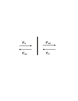
FIG. 1.: The mirror scatters the two counterpropagating fields.

The matrix $\overline{S}$ is supposed to obey the following conditions [4]: it is real in the temporal domain, causal and unitary ($\overline{S}=\overline{S}^{\rm T}$)

$$\overline{S}[-\omega]=\overline{S}[\omega]^{*}$$

$$\overline{S}[\omega]{\rm\ is\ analytic\ and\ regular\ for\ }\mathop{\rm Im}\omega>0$$

$$\overline{S}[\omega]\overline{S}[\omega]^{\dagger}=1$$

Finally, the mirror is supposed transparent at high frequencies

$$\overline{S}[\omega]\rightarrow I{\rm\quad for\ }\omega\rightarrow\infty$$ (16)

This assumption will allow regularization of the ultraviolet divergences associated with the infiniteness of the vacuum energy. It must be noted that the perfect mirror ($s=0$ and $r=-1$ at all frequencies) does not obey this condition. So, it will be preferable to consider the perfect mirror as the limit of a model obeying the transparency condition (for example a mirror perfectly reflecting at frequencies below a reflection cutoff).

Mean radiation pressure upon a motionless mirror

The force $F(t)$ may be evaluated as the difference between the radiation pressures exerted upon the left and right sides of the mirror at rest at $q=0$. In a 2D spacetime, the component $T_{xx}$ of the stress tensor is equal to the energy density and one gets

$\displaystyle F(t)=\varphi_{\rm in}^{\prime\ 2}(t)+\psi_{\rm out}^{\prime\ 2}(t)-\varphi_{\rm out}^{\prime\ 2}(t)-\psi_{\rm in}^{\prime\ 2}(t)$

This force can also be considered as the difference between the impulsion densities of the input and output fields evaluated at the mirror’s position

$$F(t)=p_{\rm in}(t)-p_{\rm out}(t)$$ (17)

For a perfect mirror, the force is twice the impulsion density which would exist at the location of the mirror in its absence [9]. The mean value of this force is zero in the vacuum state. However, we shall see later on that the instantaneous radiation pressure has irreducible quantum fluctuations.

For a partly transmitting mirror, the force $F(t)$ is still given by the difference (10) between the input and output impulsion densities but we have now to evaluate the output fields by using the input output relation (8)

$\displaystyle C_{\rm out}[\omega,\omega^{\prime}]=\overline{S}[\omega]C_{\rm in}[\omega,\omega^{\prime}]\overline{S}[\omega^{\prime}]$

One gets an expression of the force having the same form as equation (5)

$\displaystyle\left\langle F(t)\right\rangle=\int\frac{{\rm d}\omega}{2\pi}\int\frac{{\rm d}\omega^{\prime}}{2\pi}e^{-i\omega t-i\omega^{\prime}t}i\omega i\omega^{\prime}\mathop{\rm Tr}\left[{\cal F}[\omega,\omega^{\prime}]C_{\rm in}[\omega,\omega^{\prime}]\right]$

where ${\cal F}$ is a square matrix

$${\cal F}[\omega,\omega^{\prime}] = \eta-\overline{S}[\omega^{\prime}]\eta\overline{S}[\omega]=\left(\begin{array}[]{cc}\alpha[\omega,\omega^{\prime}]&\beta[\omega,\omega^{\prime}]\\ -\beta[\omega,\omega^{\prime}]&-\alpha[\omega,\omega^{\prime}]\end{array}\right)$$ (20)

$$\alpha[\omega,\omega^{\prime}] = 1-\overline{s}[\omega]\overline{s}[\omega^{\prime}]+\overline{r}[\omega]\overline{r}[\omega^{\prime}]$$ (21)

$$\beta[\omega,\omega^{\prime}] = \overline{s}[\omega]\overline{r}[\omega^{\prime}]-\overline{r}[\omega]\overline{s}[\omega^{\prime}]$$ ()

The matrix ${\cal F}$ obeys the following properties which will be used thereafter

$${\cal F}[\omega,\omega^{\prime}]^{\rm T} = {\cal F}[\omega^{\prime},\omega]=\eta{\cal F}[\omega,\omega^{\prime}]\eta$$ ()

$${\cal F}[\omega,\omega^{\prime}]^{\dagger} = {\cal F}[-\omega^{\prime},-\omega]$$ ()

$${\cal F}[\omega,\omega^{\prime}]{\cal F}[\omega,\omega^{\prime}]^{\dagger} = {\cal F}[\omega,\omega^{\prime}]\eta+\eta{\cal F}[\omega,\omega^{\prime}]^{\dagger}$$ ()

$${\cal F}[\omega,\omega^{\prime}]^{\dagger}{\cal F}[\omega,\omega^{\prime}] = \eta{\cal F}[\omega,\omega^{\prime}]+{\cal F}[\omega,\omega^{\prime}]^{\dagger}\eta$$ ()

Using equations (7), the force is written in terms of the field anticommutators

$$\left\langle F(t)\right\rangle=\int\frac{{\rm d}\omega}{2\pi}\int\frac{{\rm d}\omega^{\prime}}{2\pi}e^{-i\omega t-i\omega^{\prime}t}i\omega i\omega^{\prime}\mathop{\rm Tr}\left[{\cal F}[\omega,\omega^{\prime}]C_{+,{\rm in}}[\omega,\omega^{\prime}]\right]$$ (22)

The force may be written in the temporal domain

$\displaystyle\left\langle F(t)\right\rangle=\left\{\partial_{t}\partial_{t^{\prime}}\mathop{\rm Tr}\left[\eta C_{\rm in}(t,t^{\prime})-\eta C_{\rm out}(t,t^{\prime})\right]\right\}_{t^{\prime}=t}$

with

$$\mathop{\rm Tr}\left[\eta C_{\rm in}(t,t^{\prime})-\eta C_{\rm out}(t,t^{\prime})\right] = {\int}{\rm d}t^{\prime\prime}{\int}{\rm d}t^{\prime\prime\prime}\mathop{\rm Tr}\left[{\cal F}(t^{\prime\prime},t^{\prime\prime\prime})C_{\rm in}(t-t^{\prime\prime},t^{\prime}-t^{\prime\prime\prime})\right]$$ (23)

$${\cal F}(t,t^{\prime}) = \delta(t^{\prime})\eta\delta(t)-\overline{S}(t^{\prime})\eta\overline{S}(t)$$ ()

It clearly appears on these expressions that the force exerted upon the mirror is a retarded function of the input stress tensor: $\overline{S}$ is a causal function and ${\cal F}(t,t^{\prime})$ is zero as soon as $t<0$ or $t^{\prime}<0$.

The expression (14) provides the mean force for any input state. For a stationary input (see equation 6), one gets a simpler expression

$\displaystyle\left\langle F\right\rangle=\int\frac{{\rm d}\omega}{2\pi}\omega^{2}\mathop{\rm Tr}\left[{\cal F}(\omega,-\omega)c_{+,{\rm in}}[\omega]\right]$

One can evaluate also the energy exchange between the field and the mirror; it is the difference between the energy densities of the input and output fields

$\displaystyle G(t)=e_{\rm in}(t)-e_{\rm out}(t)$

One finds that $G$ is given by equation (14) with ${\cal F}$ replaced by

$\displaystyle{\cal G}[\omega,\omega^{\prime}]=I-\overline{S}[\omega^{\prime}]\overline{S}[\omega]$

As $\overline{S}$ is unitary

$\displaystyle{\cal G}(\omega,-\omega)=0$

Therefore, the energy exchange is zero in any stationary state

$$\left\langle G\right\rangle=\int\frac{{\rm d}\omega}{2\pi}\omega^{2}\mathop{\rm Tr}\left[{\cal G}(\omega,-\omega)c_{\rm in}[\omega]\right]=0$$ (24)

Scattering upon a moving mirror

At perfect reflection, the field is still zero on a moving mirror [9] and the input output relations have a simple form for the fields evaluated along the mirror’s trajectory

$$\psi_{\rm out}(t+q_{t})=-\varphi_{\rm in}(t-q_{t}) \varphi_{\rm out}(t-q_{t})=-\psi_{\rm in}(t+q_{t})$$

$$\overline{\psi}_{\rm out}(\tau)=-\overline{\varphi}_{\rm in}(\tau) \overline{\varphi}_{\rm out}(\tau)=-\overline{\psi}_{\rm in}(\tau)$$

$$\overline{\Phi}_{\rm out}[\omega] = \left(\begin{array}[]{cc}0&-1\\ -1&0\end{array}\right)\overline{\Phi}_{\rm in}[\omega]$$

These relations describe the Doppler shift associated with the mirror’s motion (Lorentz transformation for the frequencies) and the dilatation of the derived fields $\varphi^{\prime}$ and $\psi^{\prime}$ (Lorentz transformation for the fields) [9].

For a partly transmitting mirror, the $S-$matrix (defined previously for a motionless mirror) describes the scattering of the field evaluated along the trajectory

$\displaystyle\overline{\Phi}_{\rm out}[\omega]=\overline{S}[\omega]\overline{\Phi}_{\rm in}[\omega]$

The $S-$matrix is deduced in a first order expansion in a mirror’s displacement $\delta q_{t}$ by using the transformation (4)

$$\Phi_{\rm out}[\omega]={\int}\frac{{\rm d}\omega^{\prime}}{2\pi}\left(2\pi\delta(\omega-\omega^{\prime})\overline{S}[\omega]+\delta S[\omega,\omega^{\prime}]\right)\Phi_{\rm in}[\omega^{\prime}]$$ (26)

$$\delta S[\omega,\omega^{\prime}]=i\omega^{\prime}\delta q[\omega-\omega^{\prime}]\left(\overline{S}[\omega]\eta-\eta\overline{S}[\omega^{\prime}]\right)$$ ()

Force exerted upon a moving mirror

Taking the mirror’s motion into account, the force can be written as

$\displaystyle\left\langle F(t)\right\rangle=\left\langle p_{q_{t},{\rm in}}(t)-p_{q_{t},{\rm out}}(t)\right\rangle-q_{t}^{\prime}\left\langle e_{q_{t},{\rm in}}(t)-e_{q_{t},{\rm out}}(t)\right\rangle$

where the densities are evaluated at the mirror’s position. In a first order expansion in $\delta q_{t}$, it becomes

$$\left\langle F(t)\right\rangle = \left\langle p_{\rm in}(t)-p_{\rm out}(t)\right\rangle-\delta q_{t}\partial_{t}\left\langle G(t)\right\rangle-\delta q_{t}^{\prime}\left\langle G(t)\right\rangle$$

$$\left\langle G(t)\right\rangle = \left\langle e_{\rm in}(t)-e_{\rm out}(t)\right\rangle$$

where the densities are evaluated at $x=0$, the second term represents the variation of the impulsion densities in a translation (for a free field $\partial_{x}p+\partial_{t}e=0$) and the third term is the correction proportional to energy densities and to the mirror’s velocity. The energy modification $\left\langle G(t)\right\rangle$ has to be evaluated at the zeroth order. From now on, we will restrict ourselves to stationary inputs, in which case $\left\langle G(t)\right\rangle$ is zero (see equation 16). The two corrections associated with it will be forgotten in the expression of $\left\langle F(t)\right\rangle$.

We will eventually compute the mean force as

$\displaystyle\left\langle\delta F(t)\right\rangle=-\left\langle\delta p_{\rm out}(t)\right\rangle=-\left\{\partial_{t}\partial_{t^{\prime}}\mathop{\rm Tr}\left[\eta\delta C_{\rm out}(t,t^{\prime})\right]\right\}_{t=t^{\prime}}$

where the variations of the output fields are due to the modification $\delta S$ of the $S-$matrix in the laboratory

$$\left\langle\delta F(t)\right\rangle = \int\frac{{\rm d}\omega}{2\pi}\int\frac{{\rm d}\omega^{\prime}}{2\pi}e^{-i\omega t-i\omega^{\prime}t}\omega\omega^{\prime}\mathop{\rm Tr}\left[\eta\delta C_{\rm out}[\omega,\omega^{\prime}]\right]$$

$$\delta C_{\rm out}[\omega,\omega^{\prime}] = \int\frac{{\rm d}\omega^{\prime\prime}}{2\pi}\left(\delta S[\omega,\omega^{\prime\prime}]C_{\rm in}[\omega^{\prime\prime},\omega^{\prime}]\overline{S}[\omega^{\prime}]^{\rm T}+\overline{S}[\omega]C_{\rm in}[\omega,\omega^{\prime\prime}]\delta S[\omega^{\prime},\omega^{\prime\prime}]^{\rm T}\right)$$

that is, for a stationary input (see equations 6 and 17)

$$\delta C_{\rm out}[\omega,\omega^{\prime}] = -i\omega^{\prime}\delta q[\omega+\omega^{\prime}]\left(\overline{S}[\omega]\eta-\eta\overline{S}[-\omega^{\prime}]\right)c_{\rm in}[-\omega^{\prime}]\overline{S}[\omega^{\prime}]$$ ()

$$-i\omega\delta q[\omega+\omega^{\prime}]\overline{S}[\omega]c_{\rm in}[\omega]\left(\eta\overline{S}[\omega^{\prime}]-\overline{S}[-\omega]\eta\right)$$

Using the unitarity of $\overline{S}$, one obtains

$\displaystyle\mathop{\rm Tr}\left[\eta\delta C_{\rm out}[\omega,\omega^{\prime}]\right]=\delta q[\omega+\omega^{\prime}]\mathop{\rm Tr}\left[{\cal F}[\omega,\omega^{\prime}]\left(i\omega c_{\rm in}[\omega]\eta+i\omega^{\prime}\eta c_{\rm in}[-\omega^{\prime}]\right)\right]$

We will write the motional force as a symmetric integral over the two frequencies

$$\left\langle\delta F(t)\right\rangle = \int\frac{{\rm d}\omega}{2\pi}\int\frac{{\rm d}\omega^{\prime}}{2\pi}e^{-i\omega t-i\omega^{\prime}t}\chi[\omega,\omega^{\prime}]\delta q[\omega+\omega^{\prime}]$$

$$\chi[\omega,\omega^{\prime}] = \frac{\omega\omega^{\prime}}{2}\mathop{\rm Tr}\left[{\cal F}[\omega,\omega^{\prime}]\left(i\omega c_{\rm in}[\omega]\eta+i\omega^{\prime}\eta c_{\rm in}[-\omega^{\prime}]\right)+{\cal F}[\omega^{\prime},\omega]\left(i\omega^{\prime}c_{\rm in}[\omega^{\prime}]\eta+i\omega\eta c_{\rm in}[-\omega]\right)\right]$$

Transposing the matrices inside the second line and using the properties (12), one transforms $\chi[\omega,\omega^{\prime}]$ into a function of the anticommutators (see equation 7)

$$\chi[\omega,\omega^{\prime}] = \omega\omega^{\prime}\mathop{\rm Tr}\left[{\cal F}[\omega,\omega^{\prime}]\left(i\omega c_{+,{\rm in}}[\omega]\eta+i\omega^{\prime}\eta c_{+,{\rm in}}[-\omega^{\prime}]\right)\right]$$ (28)

$$= \omega\omega^{\prime}\mathop{\rm Tr}\left[{\cal F}[\omega,\omega^{\prime}]i\omega c_{+,{\rm in}}[\omega]\eta+{\cal F}[\omega^{\prime},\omega]i\omega^{\prime}c_{+,{\rm in}}[\omega^{\prime}]\eta\right]$$ ()

Finally, the force appears as a linear response to the mirror’s motion

$$\left\langle\delta F[\omega]\right\rangle=\chi[\omega]\delta q[\omega]$$ (29)

with a susceptibility given by

$$\chi[\omega]=\int\frac{{\rm d}\omega^{\prime}}{2\pi}\chi[\omega^{\prime},\omega-\omega^{\prime}]$$ (30)

These expressions generalize the motional force (1) known for a perfect mirror in the vacuum to the case of a partly transmitting mirror in an arbitrary stationary input field. Later on, we shall see that the force (1) is recovered as an approximate result.

We have shown that the motional force is a consequence of the transformation of the fields by the moving mirror. Actually, this transformation is a squeezing effect: the particular case where the input state is the vacuum is discussed later on. In order to squeeze the field, the mirror has to exchange energy with it. A motional force thus appears as the signature of the squeezing effect.

Interpretation of the motional force in the comoving frame

It is instructive to compute the force in the comoving frame

$\displaystyle\left\langle\overline{F}(\tau)\right\rangle=\left\langle\overline{p}_{\rm in}(\tau)-\overline{p}_{\rm out}(\tau)\right\rangle=\left\{\partial_{\tau}\partial_{\tau^{\prime}}\mathop{\rm Tr}\left[\eta\overline{C}_{\rm in}(\tau,\tau^{\prime})-\eta\overline{C}_{\rm out}(\tau,\tau^{\prime})\right]\right\}_{\tau=\tau^{\prime}}$

This expression differs from the force computed in the laboratory but the corrections are seen to depend upon the energy exchange $\left\langle\overline{G}(\tau)\right\rangle$ and they can be forgotten (see the previous discussion). The mean force is the same in the laboratory or in the comoving frame in a first order expansion in $\delta q_{t}$.

In the comoving frame, one can use the expression of the force computed for a motionless mirror but the input stress tensor has to be modified because of the mirror’s motion

$\displaystyle\left\langle\delta\overline{F}(t)\right\rangle=\int\frac{{\rm d}\omega}{2\pi}\int\frac{{\rm d}\omega^{\prime}}{2\pi}e^{-i\omega t-i\omega^{\prime}t}i\omega i\omega^{\prime}\mathop{\rm Tr}\left[{\cal F}[\omega,\omega^{\prime}]\delta\overline{C}_{\rm in}[\omega,\omega^{\prime}]\right]$

The apparent stress tensor is obtained from the transformation (4) of the fields

$\displaystyle\delta\overline{C}_{\rm in}(t,t^{\prime})=-\delta q_{t}\eta\partial_{t}\overline{C}_{\rm in}(t,t^{\prime})-\partial_{t^{\prime}}\overline{C}_{\rm in}(t,t^{\prime})\eta\delta q_{t^{\prime}}$

that is, for a stationary input

$$\delta\overline{C}_{\rm in}[\omega,\omega^{\prime}]=\delta q[\omega+\omega^{\prime}]\left(-i\omega c_{\rm in}[\omega]\eta-i\omega^{\prime}\eta c_{\rm in}[-\omega^{\prime}]\right)$$ (31)

This gives exactly the same force as previously.

So the force exerted upon a moving mirror can be computed in the laboratory by considering that the $S-$matrix is modified (see equation 17) or in the comoving frame by considering that the input stress tensor is modified (see equation 22). It clearly appears in the comoving frame that the force is a causal function of the mirror’s trajectory (see equation 15). We will discuss this point more precisely in the particular case of a vacuum input.

Fluctuations of the radiation pressure upon a motionless mirror

The appearance of a force for a moving mirror can actually be guessed by inspecting the situation where the mirror is at rest. Indeed, we shall now exhibit the quantitative relation between the motional force and the noise spectrum of the force computed for a motionless mirror. This connection can be considered as a ‘fluctuation-dissipation’ theorem for a mirror which scatters field fluctuations. We will thus check in this context that the motional force can be deduced from linear response theory.

As a qualitative introduction to the problem of force fluctuations, we consider the expression (10) which relates the force and the impulsion densities $p_{\rm in}$ and $p_{\rm out}$ of the input and output fields. We see that the instantaneous impulsion density has irreducible quantum fluctuations. For example the two counterpropagating energy fluxes are statistically independent random variables in the vacuum state and the force fluctuations do not vanish.

We come now to a quantitative evaluation of the correlation function $C_{FF}$ of the force exerted upon a partly transmitting mirror

$\displaystyle C_{FF}(t)=\left\langle F(t)F(0)\right\rangle-\left\langle F\right\rangle^{2}$

Using the input-output relation (8), one obtains an operatorial expression of the force analogous to equation (14)

$$F(t)=\int\frac{{\rm d}\omega}{2\pi}\int\frac{{\rm d}\omega^{\prime}}{2\pi}e^{-i\omega t-i\omega^{\prime}t}i\omega i\omega^{\prime}\mathop{\rm Tr}\left[{\cal F}[\omega,\omega^{\prime}]\Phi_{\rm in}[\omega]\Phi_{\rm in}[\omega^{\prime}]^{\rm T}\right]$$ (32)

It follows that $C_{FF}$ depends upon four-points correlation functions of the fields. Inserting the expressions (2) of the input fields in terms of the annihilation and creation operators, we compute the four-points functions ($\Phi_{\alpha}$ stands for a component $\varphi$ or $\psi$ of the input field; we suppose that the input field is in a stationary Gaussian state; this is the case for the vacuum; this property is equivalent to the Wick’s rules [17])

$$\left\langle\Phi_{\alpha}[\omega]\Phi_{\beta}[\omega^{\prime}]\Phi_{\alpha^{\prime}}[\omega^{\prime\prime}]\Phi_{\beta^{\prime}}[\omega^{\prime\prime\prime}]\right\rangle-\left\langle\Phi_{\alpha}[\omega]\Phi_{\beta}[\omega^{\prime}]\right\rangle\left\langle\Phi_{\alpha^{\prime}}[\omega^{\prime\prime}]\Phi_{\beta^{\prime}}[\omega^{\prime\prime\prime}]\right\rangle$$

$$\qquad=2\pi\delta(\omega+\omega^{\prime\prime})c_{\alpha\alpha^{\prime}}[\omega]2\pi\delta(\omega^{\prime}+\omega^{\prime\prime\prime})c_{\beta\beta^{\prime}}[\omega^{\prime}]+2\pi\delta(\omega+\omega^{\prime\prime\prime})c_{\alpha\beta^{\prime}}[\omega]2\pi\delta(\omega^{\prime}+\omega^{\prime\prime})c_{\beta\alpha^{\prime}}[\omega^{\prime}]$$

The autocorrelation function of the force thus comes out as (using the properties 12)

$$C_{FF}(t) = \int\frac{{\rm d}\omega}{2\pi}\int\frac{{\rm d}\omega^{\prime}}{2\pi}e^{-i\omega t-i\omega^{\prime}t}C_{FF}[\omega,\omega^{\prime}]$$ ()

$$C_{FF}[\omega,\omega^{\prime}] = 2\omega^{2}\omega^{\prime\ 2}\mathop{\rm Tr}\left[{\cal F}[\omega,\omega^{\prime}]c_{\rm in}[\omega]{\cal F}[\omega,\omega^{\prime}]^{\dagger}c_{\rm in}[\omega^{\prime}]^{\rm T}\right]$$ ()

It appears that $C_{FF}$ is a symmetric function of the two frequencies

$\displaystyle C_{FF}[\omega,\omega^{\prime}]=C_{FF}[\omega^{\prime},\omega]$

One obtains the noise spectrum of the force as the Fourier transforms of the autocorrelation function (24)

$$C_{FF}[\omega]=\int\frac{{\rm d}\omega^{\prime}}{2\pi}C_{FF}[\omega^{\prime},\omega-\omega^{\prime}]$$ (33)

The explicit evaluation of this noise spectrum for a mirror in the vacuum will be given later on.

Commutator of the force operator

In order to exhibit the fluctuation-dissipation relations, we have to compute the mean value of the commutator of the force operator

$\displaystyle\xi_{FF}(t)=\frac{C_{FF}(t)-C_{FF}(-t)}{2\hbar}$

We write it

$$\xi_{FF}(t)=\int\frac{{\rm d}\omega}{2\pi}\int\frac{{\rm d}\omega^{\prime}}{2\pi}e^{-i\omega t-i\omega^{\prime}t}\xi_{FF}[\omega,\omega^{\prime}]$$ ()

$$\xi_{FF}[\omega,\omega^{\prime}]=\frac{C_{FF}[\omega,\omega^{\prime}]-C_{FF}[-\omega^{\prime},-\omega]}{2\hbar}$$ ()

Using the properties (12), one transforms this expression into

$\displaystyle\xi_{FF}[\omega,\omega^{\prime}]=\frac{\omega^{2}\omega^{\prime\ 2}}{\hbar}\mathop{\rm Tr}\left[{\cal F}[\omega,\omega^{\prime}]c_{\rm in}[\omega]{\cal F}[\omega,\omega^{\prime}]^{\dagger}c_{\rm in}[\omega^{\prime}]^{\rm T}-{\cal F}[\omega,\omega^{\prime}]c_{\rm in}[-\omega]^{\rm T}{\cal F}[\omega,\omega^{\prime}]^{\dagger}c_{\rm in}[-\omega^{\prime}]\right]$

One then writes the covariances in terms of anticommutators and commutators (see equations 7)

$\displaystyle\xi_{FF}[\omega,\omega^{\prime}]=\frac{\omega\omega^{\prime}}{2}\mathop{\rm Tr}\left[{\cal F}[\omega,\omega^{\prime}]\omega c_{+,{\rm in}}[\omega]{\cal F}[\omega,\omega^{\prime}]^{\dagger}+{\cal F}[\omega,\omega^{\prime}]{\cal F}[\omega,\omega^{\prime}]^{\dagger}\omega^{\prime}c_{+,{\rm in}}[\omega^{\prime}]^{\rm T}\right]$

We could have derived this expression directly from the field commutators. Therefore, it is correct even when the input fields are not Gaussian variables.

Finally, one uses the property (13) to obtain (compare with the expression 19)

$$\xi_{FF}[\omega,\omega^{\prime}]=\frac{\chi[\omega,\omega^{\prime}]-\chi[-\omega,-\omega^{\prime}]}{2i}$$ (34)

A comparison with equation (28) shows that there is a connection between the force fluctuations computed for a motionless mirror and the mean force computed for a moving mirror.

Fluctuation-dissipation relation

Defining the Fourier transforms of the force commutator (27)

$$\xi_{FF}[\omega]=\int\frac{{\rm d}\omega^{\prime}}{2\pi}\xi_{FF}[\omega^{\prime},\omega-\omega^{\prime}]$$ (35)

one deduces from equations (28) and (29)

$$\xi_{FF}[\omega]=\frac{C_{FF}[\omega]-C_{FF}[-\omega]}{2\hbar}=\frac{\chi[\omega]-\chi[-\omega]}{2i}$$ (36)

This constitutes the fluctuation-dissipation relation for a mirror submitted to the radiation pressure of scattered field fluctuations.

This establishes that the motional force can be derived from the correlation functions using the linear response theory. Considering that a classical modification $\delta q_{t}$ of the mirror’s trajectory corresponds to an effective perturbation of the Hamiltonian

$$\delta H(t)=-F(t)\delta q_{t}$$ (37)

where $F(t)$ is the force operator, we get the motional force (20) by using the formulas of linear response theory given in the appendix. The susceptibility $\chi[\omega]$ is actually the retarded response function while the function $\xi_{FF}[\omega]$ is the spectral density associated with the effective perturbation (32).

The fluctuation-dissipation relation (31) provides the spectral density $\xi_{FF}$ as soon as the noise spectrum or the susceptibility is known. Using the analytic properties of the response functions, the latter can therefore be deduced from the noise spectrum. The force for a moving mirror can always be guessed by inspecting the fluctuations of the force upon a motionless mirror.

The converse is not true in general. However, if the input state corresponds to a thermal equilibrium, the anticommutator of the force (the fluctuations) can be obtained from the commutator (the susceptibility). The vacuum state is the equilibrium state at zero temperature and the noise spectrum $C_{FF}$ can effectively be deduced in this case from the spectral density $\xi_{FF}$, as we see now.

The case of vacuum fluctuations

The covariance matrix corresponding to the vacuum state is easily derived from the expressions (2) of the fields in terms of the annihilation and creation operators

$\displaystyle c_{\rm vac}(\omega)=I\theta(\omega)\frac{\hbar}{2\omega}\qquad c_{+,{\rm vac}}(\omega)=I\frac{\hbar}{4\left|\omega\right|}$

This covariance matrix is scalar so that the mean radiation pressure (14) is zero as expected.

The function $\chi$ (see equation 19) corresponding to the vacuum is

$\displaystyle\chi_{\rm vac}[\omega,\omega^{\prime}]=\frac{i\hbar}{2}\omega\omega^{\prime}\left(\varepsilon(\omega)+\varepsilon(\omega^{\prime})\right)\alpha[\omega,\omega^{\prime}]$

where $\varepsilon$ is the sign function

$\displaystyle\varepsilon(\omega)=\theta(\omega)-\theta(-\omega)$

and $\alpha$ the diagonal term of the matrix ${\cal F}$ (see equation 11). It follows that the susceptibility for a mirror which scatters the vacuum fluctuations may be written (see equation 21)

$$\chi_{\rm vac}[\omega]=i\hbar\int_{0}^{\omega}\frac{{\rm d}\omega^{\prime}}{2\pi}\omega^{\prime}(\omega-\omega^{\prime})\alpha[\omega^{\prime},\omega-\omega^{\prime}]$$ (38)

If the frequency $\omega$ is such that $s=0$ and $r=-1$ between $0$ and $\omega$, $\alpha$ may be replaced by $2$ in equation (33) and the response function reduces to

$$\chi_{\rm vac}[\omega]=i\hbar\frac{\omega^{3}}{6\pi}$$ (39)

This means that the damping force in the vacuum can be approximated by equation (1), in the limiting case of a perfect mirror, at frequencies below the reflection cutoff. In other words, the coarse grained force (force averaged over a time longer than the reflection delay) is proportional to $q^{\prime\prime\prime}$. However, it has to be emphasized that the exact expression (33) is causal which is not the case for the approximated one (34). Regularized and causal expressions are obtained only when considering partly transmitting mirrors [4].

The force (1) is identical to the linear approximation (first order expansion in the mirror’s displacement $\delta q$) of the non linear expression obtained by Fulling and Davies for a perfectly reflecting mirror [8]. It is worth to note that it is also the non relativistic limit ($q^{\prime}\ll c=1$) of this expression. This suggests that the domain of validity of the first-order expansion corresponds to a non-relativistic mirror velocity.

The vacuum fields may be considered as Gaussian random variables [17] so that we can effectively compute the force correlations from the field covariance matrix. One gets from equations (25) and (13)

$\displaystyle C_{FF,{\rm vac}}[\omega,\omega^{\prime}]=\hbar^{2}\theta(\omega)\theta(\omega^{\prime})\omega\omega^{\prime}\left(\alpha[\omega,\omega^{\prime}]+\alpha[\omega,\omega^{\prime}]^{*}\right)$

One then deduces the noise spectrum of the force

$$C_{FF,{\rm vac}}[\omega]=2\hbar\theta(\omega)\xi_{FF,{\rm vac}}[\omega]\qquad\xi_{FF,{\rm vac}}[\omega]=\frac{\chi_{\rm vac}[\omega]-\chi_{\rm vac}[-\omega]}{2i}$$ (40)

Clearly, the fluctuation-dissipation relation is obeyed in the vacuum state. Simple results are obtained when the reflection is perfect at frequencies between 0 and $\omega$

$$C_{FF,{\rm vac}}[\omega] = \frac{\hbar^{2}}{3\pi}\theta(\omega)\omega^{3}$$ ()

$$\xi_{FF,{\rm vac}}[\omega] = \frac{\hbar}{6\pi}\omega^{3}$$ ()

The connection between the variation of $C_{FF}$ as $\omega^{3}$ and the variation of the damping force as $q^{\prime\prime\prime}$ is a manifestation of the fluctuation-dissipation relation. As already noted, the noise spectrum (35) is more regular at high frequencies than the approximation (36) as a consequence of the transparency condition (9).

Two properties of the noise spectrum (35) have to be emphasized. First, $C_{FF}$ is zero at the limit of a null frequency, which means that the force fluctuations are averaged to zero when integrated over a long time. Note that the input impulsion density $p_{\rm in}$ also vanishes when integrated over a long time.

Second, the relation (35) between the noise spectrum $C_{FF}$ and the spectral density $\xi_{FF}$ implies that the noise spectrum contains only positive frequency components, because the vacuum is the zero temperature state. It follows that the vacuum can damp the mirror’s motion but cannot excite it.

Connection with squeezing

We have developed a formalism where the scattering is characterized by frequency dependent coefficients. The effect of the mirror’s motion is described by a modification of the $S-$matrix in the laboratory or by a transformation of the input stress tensor in the comoving frame. It can be noted that the scattering formalism has already been used for dealing with vacuum fluctuations in accelerated frames or in curved space [18, 19, 20, 21, 22, 23].

In this scattering approach, the damping force for a mirror in the vacuum appears as connected to squeezing [24, 25]. In order to put this point into evidence, we write the secular part (component at zero frequency) of the effective Hamiltonian (32) as follows (see the operatorial expression 23 of the force)

$\displaystyle\delta H[0]={\int}{\rm d}t\ \delta H(t)=\int\frac{{\rm d}\omega}{2\pi}\int\frac{{\rm d}\omega^{\prime}}{2\pi}\delta q[-\omega-\omega^{\prime}]\omega\omega^{\prime}\mathop{\rm Tr}\left[{\cal F}[\omega,\omega^{\prime}]\Phi_{\rm in}[\omega]\Phi_{\rm in}[\omega^{\prime}]^{\rm T}\right]$

Considering as an example the case where the mirror oscillates at a fixed frequency 2$\omega_{0}$

$\displaystyle\delta q_{t}=\delta q_{0}\cos(2\omega_{0}t)$

one recognizes an effective Hamiltonian giving rise to a squeezing effect [1].

Actually, the motional force constitutes a mechanical consequence of the squeezing. As the input field is the vacuum state, the mirror has to give energy to the field in order to squeeze it and this damps its motion.

In the laboratory frame, the modification of the output covariance matrix which results from the effective Hamiltonian is given by equation (18)

$\displaystyle\delta C_{\rm out}[\omega,\omega^{\prime}]=\frac{i\hbar}{2}\delta q[\omega+\omega^{\prime}]\left(\theta(\omega)-\theta(-\omega^{\prime})\right){\cal F}[\omega^{\prime},\omega]$

For the oscillating mirror, this is non zero only if the two frequencies $\omega$ and $\omega^{\prime}$ have the same sign and if their sum is $\pm 2\omega_{0}$. It follows that the squeezing effect vanishes when the oscillation frequency goes to zero. A mirror moving slowly in the vacuum does not appreciably squeeze it and the motional force (1) is very small at low frequencies.

The connection of the motional force with squeezing can be analysed also in the comoving frame. Now, the apparent input state (22) is itself squeezed when the input is the vacuum in the laboratory frame. The motional force thus appears as a mechanical manifestation of the fact that the mirror scatters (with the unmodified $S-$matrix) squeezed field fluctuations.

Conclusion

We have given the explicit expressions of the correlation functions and of the motional force experienced by a mirror in the vacuum state. When the mirror is irradiated by a coherent wave, the same method leads to a mean radiation pressure and to extra fluctuations [15]. It also provides an extra damping force, proportional to the mirror’s velocity and to the coherent field intensity [16]. These two results are related through the fluctuation-dissipation theorem which would hold also for a mirror in a thermal field.

We have only considered in this paper the one mirror problem. The situation where two mirrors scatter the same field fluctuations seems attractive. The mean Casimir force is well known for motionless mirrors. It is expected to be modified when the mirrors are moving [7, 8]. It must also exhibit fluctuations [26]. These fluctuations have to be connected with the motional effect in the same manner as in the one mirror problem. Finally, the motional dependence of the Casimir effect is associated to the squeezing effect due to the mirrors’ motion. The formalism developed in the present paper is applied to the two-mirrors problem in a forthcoming paper.

Acknowlegdements

We thank C.Fabre, E.Giacobino and A.Heidmann for discussions.

A The relations of linear response theory

A classical modification $\delta q_{t}$ of the mirror’s trajectory corresponds to an effective perturbation (32) of the Hamiltonian. The linear response theory [6] provides the variation of the mean force

$\displaystyle\left\langle\delta F(t)\right\rangle={\int}{\rm d}t^{\prime}\ \chi_{FF}^{R}(t-t^{\prime})\delta q(t^{\prime})$

The response function $\chi_{FF}^{R}$ (the abbreviated notation $\chi$ was used previously) is the retarded susceptibility; it is related to the force commutator $\xi_{FF}$ and to the correlation function $C_{FF}$ (correlation functions are supposed stationary)

$\displaystyle\chi_{FF}^{R}(t)=2i\theta(t)\xi_{FF}(t)\qquad\xi_{FF}(t)=\frac{C_{FF}(t)-C_{FF}(-t)}{2\hbar}\qquad C_{FF}(t)=\left\langle F(t)F(0)\right\rangle-\left\langle F\right\rangle^{2}$

It is also possible to define an advanced response

$\displaystyle\chi_{FF}^{A}(t)=-2i\theta(-t)\xi_{FF}(t)=\chi_{FF}^{R}(-t)$

These relations have a simple form in the spectral domain

$$\left\langle\delta F[\omega]\right\rangle = \chi_{FF}^{R}[\omega]\delta q[\omega]\qquad\chi_{FF}^{R}[\omega]=\widetilde{\xi}_{FF}[\omega]+i\xi_{FF}[\omega]$$

$$\chi_{FF}^{A}[\omega] = \widetilde{\xi}_{FF}[\omega]-i\xi_{FF}[\omega]=\chi_{FF}^{R}[\omega]^{*}=\chi_{FF}^{R}[-\omega]$$

The dispersive part $\widetilde{\xi}_{FF}$ of the susceptibility functions is obtained from the spectral density $\xi_{FF}$ through a dispersion relation

$\displaystyle\widetilde{\xi}_{FF}[\omega]=\int\frac{{\rm d}\omega^{\prime}}{\pi}P\frac{\xi_{FF}[\omega^{\prime}]}{\omega^{\prime}-\omega}$

The response function $\chi_{FF}^{R}$ (respectively $\chi_{FF}^{A}$) is analytic (and regular) in the upper half plane $\mathop{\rm Im}\omega>0$ (respectively in the lower half plane $\mathop{\rm Im}\omega<0$). As $F$ is a Hermitean operator, $\xi_{FF}$ is a real and odd function of $\omega$ while $\widetilde{\xi}_{FF}$ is a real and even function of $\omega$.

The general form of the relation between the noise spectrum $C_{FF}$ and the retarded susceptibility $\chi_{FF}^{R}$ is

$\displaystyle\xi_{FF}(t)=\frac{C_{FF}(t)-C_{FF}(-t)}{2\hbar}=\frac{\chi_{FF}^{R}(t)-\chi_{FF}^{R}(-t)}{2i}$

which leads to equation (31) in the frequency domain

$\displaystyle\xi_{FF}[\omega]=\frac{C_{FF}[\omega]-C_{FF}[-\omega]}{2\hbar}=\frac{\chi_{FF}^{R}[\omega]-\chi_{FF}^{R}[-\omega]}{2i}$

REFERENCES

• [1] ‘Squeezed Light’ , eds Loudon and Knight, J. Mod. Opt. 34 709-1020 (1987); ‘Squeezed States of the Electromagnetic Field’ , eds Kimble and Walls, J. Opt. Soc. Am. B4 1449-1741 (1987); Squeezed and non classical Light , eds Tombesi and Pike, Plenum (New York, 1989).
• [2] Casimir H.B.G., Proc. K. Ned. Akad. Wet. 51 793 (1948).
• [3] Plunien G., Müller B. and Greiner W., Phys. Rep. 134 87 (1986).
• [4] Jaekel M.T. and Reynaud S., J. Physique I 1 1395 (1991).
• [5] Ford G.W., Kac M. and Mazur P., J. Math. Phys. 6 504 (1965); Mori H., Prog. Theor. Phys. 33 423 (1965); Gardiner C.W., IBM J. Res. Dev. 32 127 (1988).
• [6] Kubo R., Rep. Prog. Phys. 29 255 (1966).
• [7] De Witt B.S., Phys. Rep. 19 295 (1975).
• [8] Fulling S.A. and Davies P.C.W., Proc. R. Soc. A348 393 (1976).
• [9] Moore G.T., J. Math. Phys. 11 2679 (1970).
• [10] Razavy M. and Terning J., Phys. Rev. D31 307 (1985).
• [11] Quantum Optics, Experimental Gravitation and Measurement Theory , eds Meystre and Scully (Plenum, New York, 1983).
• [12] Brillet A., Damour T. and Tourrenc Ph., Ann. Physique 10 201 (1985); Brillet A., Ann. Physique 10 219 (1985).
• [13] Gea-Banacloche J. and Leuchs G., J. Opt. Soc. Am. B4 1667 (1987); Gea-Banacloche J. and Leuchs G., J. Mod. Opt. 34 793 (1987).
• [14] Jaekel M.T. and Reynaud S., EuroPhys. Lett. 13 301 (1990).
• [15] Caves C.M., Phys. Rev. Lett. 45 75 (1980).
• [16] Unruh W.G. in ref. [11] p.647.
• [17] Itzykson C. and Zuber J.B., Quantum Field Theory (Mc Graw Hill, New York, 1980).
• [18] Rindler W., Am. J. Phys. 34 1174 (1966).
• [19] Hawkins S.W., Commun. Math. Phys. 43 199 (1975).
• [20] Davies P.C.W., J. Phys. A8 609 (1975).
• [21] Unruh W.G., Phys. Rev. D14 870 (1976).
• [22] Davies P.C.W. and Fulling S.A., Proc. R. Soc. A354 59 (1977).
• [23] Birrell N.D. and Davies P.C.W., Quantum fields in curved space (Cambridge University Press, Cambridge, 1989).
• [24] Sarkar S., in Photons and quantum fluctuations, eds E.R.Pike and H.Walther, (Adam Hilger, London, 1988) p. 151.
• [25] Dodonov V.V., Klimov A.B. and Man’Ko V.I., Phys. Lett. A149 225 (1990).
• [26] Barton G., J. Phys. A24 991 (1991).