Casimir force between partially transmitting mirrors

Abstract

The Casimir force can be understood as resulting from the radiation pressure exerted by the vacuum fluctuations reflected by boundaries. We extend this local formulation to the case of partially transmitting boundaries by introducing reflectivity and transmittivity coefficients obeying conditions of unitarity, causality and high frequency transparency. We show that the divergences associated with the infiniteness of the vacuum energy do not appear in this approach. We give explicit expressions for the Casimir force which hold for any frequency dependent scattering and any temperature. The corresponding expressions for the Casimir energy are interpreted in terms of phase shifts. The known results are recovered at the limit of a perfect reflection.

PACS: 03.65 - 42.50 - 12.20

Introduction

As a consequence of Heisenberg inequalities, the electromagnetic field exhibits quantum fluctuations even in the vacuum state. These “vacuum fluctuations” have been extensively studied in the domain of quantum optics these last years [1]. Casimir [2] observed that the resulting vacuum energy ($\frac{1}{2}\hbar\omega$ per field mode) depends upon the boundary conditions and particularly upon the positions of reflecting bodies. As a consequence, the vacuum fluctuations manifest themselves through macroscopic forces.

These Casimir forces are usually computed by comparing the mode density in the absence and in the presence of perfectly reflecting boundaries [3]. In a local formulation, they can also be understood as resulting from the radiation pressure exerted by the vacuum fluctuations reflected by the boundaries [4, 5]. In the simplest case of a scalar field in a two-dimensional (2D) spacetime, one gets the following force between two pointlike mirrors at a distance $q$

$$F=\frac{\hbar c\pi}{24q^{2}}$$ (1)

For the electromagnetic field in a four-dimensional (4D) spacetime, one gets the Casimir pressure (force measured per unit area) between two parallel plane and infinite mirrors [6]

$$F=\frac{\hbar c\pi^{2}}{240q^{4}}$$ (2)

From now on, we use natural units where $c=\varepsilon_{0}=k_{\rm B}=1$; however, we keep $\hbar$ as a scale for vacuum fluctuations.

A problem in any calculation of vacuum induced effects is to dispose of the divergences associated with the infiniteness of the total vacuum energy. Usually, this is done by arbitrarily cutting off the mode density. The divergences of the energy in the absence and in the presence of the boundaries cancel each other, which leads to a finite net result at the limit of infinite cutoff frequency. In the local formulation, the field correlation function diverges when the fields are evaluated at the same point. A regularized stress tensor is obtained by splitting the two points and ignoring the divergent part [4, 7].

Clearly, a more natural regularization should be provided by studying partially transmitting mirrors. Any real mirrors are certainly transparent at high frequencies so that the expression of the force should be regular. Using the physical properties of a dielectric constant, Lifshitz [8] has obtained regular expressions for the Casimir-Polder forces between macroscopic dielectric bodies [9, 10]. This approach is not free from problems, such as the effect of dissipation and the expression of energy density in a dispersive dielectric medium, which have been discussed in detail [11, 12].

In this paper, we use a scattering approach to avoid these problems. We use the local formulation and introduce frequency dependent reflectivity and transmittivity coefficients for the two mirrors, which are assumed to obey conditions of reality, unitarity, causality and high frequency transparency. The scattering coefficients determine the vacuum stress tensor and therefore the Casimir force on the mirrors. Explicit expressions, which come out as finite integrals, are obtained for any frequency dependent scattering. Eventually, the reflectivity function appears as a physical regulator and the known results (1) and (2) are recovered when the mirrors are totally reflecting over a large enough frequency interval.

These results do not rely upon a detailed microscopic analysis of the scattering process and are not limited to dielectric mirrors. Dissipative processes are disregarded (unitary scattering) and all field fluctuations originate from the input vacuum. We also give the results for a non zero temperature input state. The Casimir energy can be deduced by integrating the force and is different from the integrated field energy when the reflectivities are frequency dependent. This expression, interpreted in terms of phase shifts, makes the connection with the mode density approach.

A first part details the simple case where two pointlike mirrors are placed in the vacuum state, or in a thermal state, of a scalar field in a 2D spacetime. We come then to the problem of parallel plane and infinite mirrors which scatter the electromagnetic field in a 4D spacetime. Following Lifshitz [8], the effect of evanescent waves is accounted for. Expressions of the forces as integrals over imaginary frequencies [8] are given in an appendix.

The following convention is used throughout the paper: any function $f(t)$ defined in the time domain and its Fourier transform $f[\omega]$ are related through

$\displaystyle f(t)=\int\frac{{\rm d}\omega}{2\pi}f[\omega]e^{-i\omega t}$

One mirror in 2D vacuum

In a 2D spacetime (one time coordinate $t$, one space coordinate $x$), a free field is the sum of two counterpropagating fields

$\displaystyle\Phi=\varphi\left(t-x\right)+\psi\left(t+x\right)$

It can also be described by a twofold column matrix in the frequency domain

$\displaystyle\Phi[\omega]=\left(\begin{array}[]{c}\varphi[\omega]\\ \psi[\omega]\end{array}\right)$

We consider now that the field is scattered by a mirror located at point $q$

$\displaystyle\Phi=\theta(q-x)\left(\varphi_{\rm in}(t-x)+\psi_{\rm out}(t+x)\right)+\theta(x-q)\left(\psi_{\rm in}(t+x)+\varphi_{\rm out}(t-x)\right)$

where $\varphi_{\rm in}$ and $\psi_{\rm in}$ are the input fields, $\varphi_{\rm out}$ and $\psi_{\rm out}$ the output fields (see Figure 1).

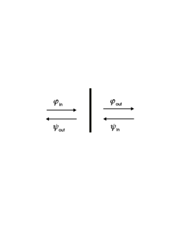
FIG. 1.: One mirror scatters the two counterpropagating fields.

With the hypothesis of a perfect reflection, the field vanishes on the mirror

$\displaystyle\varphi_{\rm out}(t)=-\psi_{\rm in}(t+2q)\qquad\psi_{\rm out}(t)=-\varphi_{\rm in}(t-2q)$

Equivalently

$\displaystyle\varphi_{\rm out}[\omega]=-\psi_{\rm in}[\omega]e^{-2i\omega q}\qquad\psi_{\rm out}[\omega]=-\varphi_{\rm in}[\omega]e^{2i\omega q}$

In the general case of a partially transmitting mirror, the scattering of the field is described by a frequency dependent $S$ matrix

$$\Phi_{\rm out}[\omega]=S[\omega]\Phi_{\rm in}[\omega]\qquad S[\omega]=\left(\begin{array}[]{cc}s[\omega]&r[\omega]e^{-2i\omega q}\\ r[\omega]e^{2i\omega q}&s[\omega]\end{array}\right)$$ (3)

We assume that the $S$ matrix obeys the following conditions. The values of $S$ are real in the temporal domain

$$s[-\omega]=s[\omega]^{*}\qquad r[-\omega]=r[\omega]^{*}$$ (4)

The scattering is causal [13]

$$s(t)=r(t)=0\ {\rm for}\ t<0$$ (5)

$$s[\omega]\ {\rm and}\ r[\omega]\ {\rm are\ analytic\ and\ regular\ for}\ \mathop{\rm Im}\omega>0$$ (6)

The scattering matrix is unitary (dissipation inside the mirror is neglected)

$$S[\omega]S[\omega]^{\dagger}=1$$ (7)

$$\left|s[\omega]\right|^{2}+\left|r[\omega]\right|^{2} = 1\qquad s[\omega]r[\omega]^{*}+r[\omega]s[\omega]^{*}=0$$ (8)

The mirror is transparent at high frequencies and the reflectivity decreases sufficiently rapidly

$$s[\omega]\rightarrow 1\qquad\omega\left|r[\omega]\right|\rightarrow 0\qquad{\rm for}\ \omega\rightarrow\infty$$ (9)

Because of the transparency condition (9), the reflectivity will provide a natural regulator to the ultraviolet divergence of the vacuum energy. The perfectly reflecting mirror corresponds to $r=-1$ and $s=0$ at all frequencies and does not obey this condition. So, it will be preferable to consider the perfect mirror as the limit of a model obeying the conditions (4-9). This amounts to consider the effect of non zero reflection delays and to let them go to zero at the end of the calculations.

Quantum field theory provides the field correlation functions corresponding to the vacuum state. We will use the symmetric correlation functions which are the mean values of the anticommutators

$$\left\langle\left\{\varphi^{\prime}(t+\tau),\varphi^{\prime}(t)\right\}\right\rangle = \left\langle\left\{\psi^{\prime}(t+\tau),\psi^{\prime}(t)\right\}\right\rangle=\frac{c(t)}{2}$$ (10)

$$\left\langle\left\{\varphi^{\prime}(t+\tau),\psi^{\prime}(t)\right\}\right\rangle = 0$$ (11)

$$\varphi^{\prime}(t) = \partial_{t}\varphi(t)$$ (12)

$$i\omega i\omega^{\prime}\left\langle\left\{\varphi[\omega],\varphi(\omega^{\prime})\right\}\right\rangle = i\omega i\omega^{\prime}\left\langle\left\{\psi[\omega],\psi(\omega^{\prime})\right\}\right\rangle=2\pi\delta(\omega+\omega^{\prime})\frac{c[\omega]}{2}$$ (13)

$$i\omega i\omega^{\prime}\left\langle\left\{\varphi[\omega],\psi(\omega^{\prime})\right\}\right\rangle = 0$$ (14)

with

$$c(\tau) = \lim_{\epsilon\rightarrow 0^{+}}\frac{\hbar}{2\pi}\left[\frac{1}{\left(\epsilon+i\tau\right)^{2}}+\frac{1}{\left(\epsilon-i\tau\right)^{2}}\right]$$ (15)

$$c[\omega] = \hbar\left|\omega\right|$$ (16)

As usual in the local formulation, one evaluates the force as the difference between the radiation pressures exerted upon the left and right sides of the mirror. In a 2D spacetime, the component $T_{xx}$ of the stress tensor is equal to the energy density and one gets

$$F=e_{\rm L}-e_{\rm R}$$ (17)

$$e_{\rm L} = \left\langle\varphi_{\rm in}^{\prime\ 2}(t-q)+\psi_{\rm out}^{\prime\ 2}(t+q)\right\rangle\qquad e_{\rm R}=\left\langle\psi_{\rm in}^{\prime\ 2}(t+q)+\varphi_{\rm out}^{\prime\ 2}(t-q)\right\rangle$$ (18)

Substituting the output fields in terms of the input fields and using the unitarity condition, one obtains

$\displaystyle\left\langle\varphi_{\rm out}^{\prime\ 2}(t-q)\right\rangle=\left\langle\psi_{\rm out}^{\prime\ 2}(t+q)\right\rangle=\left\langle\varphi_{\rm in}^{\prime\ 2}(t-q)\right\rangle=\left\langle\psi_{\rm in}^{\prime\ 2}(t+q)\right\rangle=\frac{c(0)}{4}$

Hence

$$e_{\rm L}=e_{\rm R}=\int_{0}^{\infty}\frac{{\rm d}\omega}{2\pi}c[\omega]$$ (19)

The radiation pressures exerted upon the two sides of the mirror are infinite. However, they cancel each other exactly and the net force is zero. This is connected to the property that the impulsion density is zero in the vacuum state of a free field while the energy density is infinite. Note that the cancellation between infinite quantities is obtained inside a single physical situation and not by comparing two different situations.

Two mirrors in 2D vacuum

We study now the situation where two pointlike mirrors are placed in the 2D vacuum at positions $q_{1}$ and $q_{2}$ (see Fig.2).

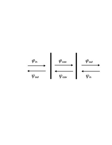
FIG. 2.: Two mirrors scatter the two counterpropagating fields.

As is usual in the theory of a Fabry Perot cavity, the global scattering may be deduced from the elementary scattering matrices given by (3) and associated with the two mirrors

$$\left(\begin{array}[]{c}\varphi_{\rm cav}[\omega]\\ \psi_{\rm out}[\omega]\end{array}\right) = \left(\begin{array}[]{cc}s_{1}[\omega]&r_{1}[\omega]e^{-2i\omega q_{1}}\\ r_{1}[\omega]e^{2i\omega q_{1}}&s_{1}[\omega]\end{array}\right)\left(\begin{array}[]{c}\varphi_{\rm in}[\omega]\\ \psi_{\rm cav}[\omega]\end{array}\right)$$

$$\left(\begin{array}[]{c}\varphi_{\rm out}[\omega]\\ \psi_{\rm cav}[\omega]\end{array}\right) = \left(\begin{array}[]{cc}s_{2}[\omega]&r_{2}[\omega]e^{-2i\omega q_{2}}\\ r_{2}[\omega]e^{2i\omega q_{2}}&s_{2}[\omega]\end{array}\right)\left(\begin{array}[]{c}\varphi_{\rm cav}[\omega]\\ \psi_{\rm in}[\omega]\end{array}\right)$$

One can solve these equations to express the outcoming and the intracavity fields in terms of the input ones

$$\Phi_{\rm out}[\omega] = S[\omega]\Phi_{\rm in}[\omega]$$

$$\Phi_{\rm cav}[\omega] = R[\omega]\Phi_{\rm in}[\omega]$$

The global scattering matrix $S[\omega]$ and the resonance matrix $R[\omega]$ are given by

$$S_{11}[\omega] = S_{22}[\omega]=\frac{s_{1}[\omega]s_{2}[\omega]}{d[\omega]}$$ (22)

$$S_{12}[\omega] = r_{2}[\omega]e^{-i\omega q}+\frac{s_{2}[\omega]^{2}r_{1}[\omega]e^{i\omega q}}{d[\omega]}$$ (23)

$$S_{21}[\omega] = r_{1}[\omega]e^{-i\omega q}+\frac{s_{1}[\omega]^{2}r_{2}[\omega]e^{i\omega q}}{d[\omega]}$$ (24)

$$R_{11}[\omega] = \frac{s_{1}[\omega]}{d[\omega]}\qquad R_{12}[\omega]=\frac{s_{2}[\omega]r_{1}[\omega]e^{-2i\omega q_{1}}}{d[\omega]}$$ (25)

$$R_{21}[\omega] = \frac{s_{1}[\omega]r_{2}[\omega]e^{2i\omega q_{2}}}{d[\omega]}\qquad R_{22}[\omega]=\frac{s_{2}[\omega]}{d[\omega]}$$ (26)

where

$\displaystyle d[\omega]=1-r[\omega]e^{2i\omega q}\qquad r[\omega]=r_{1}[\omega]r_{2}[\omega]\qquad q=q_{2}-q_{1}$

The matrices $S$ and $R$ are real in the time domain, they are causal functions and the matrix $S$ is unitary.

Substituting the output fields in terms of the input fields and using the unitarity of the matrix $S[\omega]$, one deduces that the energy densities $e_{\rm L}$ and $e_{\rm R}$, again defined by (18), are still given by (19). But the intracavity energy density $e_{\rm cav}$ is different

$$e_{\rm cav} = \left\langle\varphi_{\rm cav}^{\prime\ 2}+\psi_{\rm cav}^{\prime\ 2}\right\rangle=\int_{0}^{\infty}\frac{{\rm d}\omega}{2\pi}c[\omega]g[\omega]$$

$$g[\omega] = \frac{\left|R_{11}\right|^{2}+\left|R_{12}\right|^{2}+\left|R_{21}\right|^{2}+\left|R_{22}\right|^{2}}{2}=\frac{1-\left|r[\omega]\right|^{2}}{\left|1-r[\omega]e^{2i\omega q}\right|^{2}}$$

The function $g[\omega]$ (calculated from equation (26)) describes an enhancement (resp. suppression) of vacuum fluctuations seen inside the cavity at frequencies inside (resp. outside) the Airy peaks [14, 15]. One deduces the Casimir force as the difference between the outer and inner radiation pressures

$$F_{1}=e_{\rm L}-e_{\rm cav}=F\qquad F_{2}=e_{\rm cav}-e_{\rm R}=-F$$ (27)

$$F=\int_{0}^{\infty}\frac{{\rm d}\omega}{2\pi}c[\omega]\left(1-g[\omega]\right)$$ (28)

In the standard derivation of the Casimir force, one considers mirrors which are perfectly reflecting at all frequencies. In this case, the Airy peaks reduce to Dirac distributions

$\displaystyle 1-g[\omega]=1-\frac{\pi}{q}\sum_{n}\delta(\omega-n\frac{\pi}{q})$

The integral (28) is then regularized by introducing a cutoff in the mode density and computed by applying the Euler-Mac Laurin summation rule [6]

$\displaystyle F=\left\{\left(\frac{B_{2}}{2!}\frac{\pi^{2}}{q^{2}}\partial_{\omega}+\frac{B_{4}}{4!}\frac{\pi^{4}}{q^{4}}\partial_{\omega}^{3}+\ldots\right)\frac{\hbar\omega}{2\pi}\right\}_{\omega=0}$

where the $B_{2k}$ are the Bernouilli numbers $B_{2}=\frac{1}{6};$ $B_{4}=-\frac{1}{30};$ $\ldots$. This leads to the expression (1) of the Casimir force.

However, the introduction of a cutoff in the mode density is not necessary since the integral (28) is finite as soon as the reflectivity functions obey the conditions (4-9). One can write

$$F=\int_{0}^{\infty}\frac{{\rm d}\omega}{2\pi}c[\omega]\frac{-r[\omega]e^{2i\omega q}}{1-r[\omega]e^{2i\omega q}}+c.c.$$ (29)

As $c[\omega]$ is an even function of $\omega$, one deduces from the reality condition (4)

$$F=\int_{-\infty}^{\infty}\frac{{\rm d}\omega}{2\pi}c[\omega]\frac{-r[\omega]}{e^{-2i\omega q}-r[\omega]}$$ (30)

One obtains the force as a sum

$$F=\sum_{\ell>0}F^{(\ell)}\qquad F^{(\ell)}=-\int_{-\infty}^{\infty}\frac{{\rm d}\omega}{2\pi}e^{2\ell i\omega q}r^{\ell}[\omega]c[\omega]$$ (31)

where each term $F^{(\ell)}$ corresponds to a number $\ell$ of roundtrips inside the cavity. This term can be transformed into a convolution product in the time domain, more precisely into an integral over $\ell$ reflection delays $t_{1}$, $\ldots$ $t_{\ell}$

$$F^{(\ell)}=-\int_{0}^{\infty}{\rm d}t_{1}r(t_{1})\ldots\int_{0}^{\infty}{\rm d}t_{\ell}r(t_{\ell})c\left(2\ell q+t_{1}+\ldots+t_{\ell}\right)$$ (32)

The reflection delays are positive and the two point correlation function $c$ is evaluated at distances between the points greater than $2q$. The expression of the force comes out free from the divergences usually associated with the infiniteness of the vacuum energy and the regulator $\epsilon$ may be omitted in the expression (16) of $c$.

In the limiting case where the reflection delays ($t_{1}$, $\ldots$ $t_{\ell}$) are much shorter than the distance $q$ between the two mirrors (large distance approximation), one can neglect them in the function $c(2\ell q+t_{1}+\ldots+t_{\ell})$. It follows that the force depends only upon the reflectivities evaluated at zero frequency

$\displaystyle F=-\sum_{\ell>0}r_{0}^{\ell}c(2\ell q)\qquad r_{0}=r[0]=r_{1}[0]r_{2}[0]$

that is

$$F=\frac{\hbar}{4\pi q^{2}}\zeta_{r_{0}}(2)$$ (33)

$$\zeta_{x}(p)=\sum_{\ell=1}^{\infty}\frac{x^{\ell}}{\ell^{p}}$$ (34)

If the two mirrors are perfectly reflecting at zero frequency, one finds the expression (1) for the Casimir force $\left(\zeta_{1}(2)=\frac{\pi^{2}}{6}\right)$.

The equation (31) allows one to evaluate the correction to the limit of ideal mirrors. It can be written as a formal series

$$F^{(\ell)} = \frac{\hbar}{2\pi}\left\{-i\left(2\ell q-i\partial_{\omega}\right)^{-1}\left(\omega r[\omega]^{\ell}\right)\right\}_{\omega=0}+c.c.$$ (35)

$$= \frac{\hbar}{2\pi}\left\{\left(2\ell q-i\partial_{\omega}\right)^{-2}r[\omega]^{\ell}\right\}_{\omega=0}+c.c.$$ (36)

When $r[\omega]$ is a very flat function, one recovers the large distance approximation where the force depends upon the value $r_{0}$ evaluated at zero frequency. The terms of the formal series which depend upon the derivatives of $r[\omega]$ may be considered as corrections to this approximation.

These discussions show that the reflectivity function $r[\omega]$ plays the same role as a regulator for the mode density. However, it is a regulator obeying the conditions (4-9) which cannot be real for real frequencies. We show in the appendix that it is possible to write the force as an integral over imaginary frequencies and that $r[i\omega]$ appears as a real regulator [8].

Casimir energy

The local formulation led us to the expression of the force. One can deduce a Casimir energy ${\cal U}$ by integrating this force (see equation (27))

$${\rm d}{\cal U}=-F_{1}{\rm d}q_{1}-F_{2}{\rm d}q_{2}=F{\rm d}q$$ (37)

We want now to compute this Casimir energy and to compare it with the integrated field energy [4].

One deduces from equation (29)

$$F = \partial_{q}{\cal U\qquad U}=\int_{0}^{\infty}\frac{{\rm d}\omega}{2\pi}\frac{-\hbar\Delta[\omega]}{2}$$ (39)

$$\Delta[\omega]=i{\rm Log}\frac{1-r[\omega]e^{2i\omega q}}{1-r[\omega]^{*}e^{-2i\omega q}}$$

One deduces respectively from the reality condition (4) and from the transparency condition (9)

$\displaystyle\Delta[0]=0\qquad\omega\Delta[\omega]\rightarrow 0\qquad{\rm for\ }\omega\rightarrow\infty$

so that the energy can be written

$${\cal U}=\int_{0}^{\infty}\frac{{\rm d}\omega}{2\pi}\frac{\hbar\omega}{2}\partial_{\omega}\Delta[\omega]$$ (40)

This is the standard form for the phase shift representation of the Casimir energy [3]. Actually, one checks from the expression (24) of the $S$ matrix that

$\displaystyle\det S[\omega]=\det S_{1}[\omega]\det S_{2}[\omega]e^{i\Delta[\omega]}$

where $S_{1}[\omega]$ and $S_{2}[\omega]$ are the elementary $S$ matrices associated with the two mirrors; $\Delta[\omega]$ is the $q-$dependent part of the sum of the two phase shifts at frequency $\omega$.

Now, one gets from equation (39)

$$\partial_{\omega}\Delta[\omega] = \frac{\left(2qr[\omega]-i\partial_{\omega}r[\omega]\right)e^{2i\omega q}}{1-r[\omega]e^{2i\omega q}}+c.c.$$ (41)

$$= -\left(1-g[\omega]\right)\left(2q+\partial_{\omega}\delta\right)-g[\omega]\sin\left(2\omega q+\delta\right)\partial_{\omega}{\rm Log}\left(1-\rho^{2}\right)$$ (42)

where $\delta$ and $\rho$ are the frequency dependent phase and modulus of the reflectivity function $r$. Usually, the Casimir effect is computed for frequency independent reflectivities. In this case, one deduces that the Casimir energy ${\cal U}$ is identical to the integrated field energy [4]

$\displaystyle{\cal U}=q\left(e_{\rm cav}-e_{\rm L}\right)=-qF$

This result is compatible with the definition (37) of ${\cal U}$ since the force scales as $q^{-2}$ in this case [7]. But the reflectivities have to be frequency dependent in order to fulfill the transparency condition (9). The resulting terms in the Casimir energy can be considered as corrections associated with the reflection delays upon the mirrors.

Casimir force for non zero temperatures

Now, we derive the expression of the Casimir force for non zero temperatures [3, 4]. We suppose that the reflectivities are independent of the temperature. Therefore, we have only to change the correlation function of the input fields.

The Casimir force is given by the integrals (28) or (30) with a modified function $c$

$$c_{T}[\omega]=c_{0}[\omega]n_{T}[\omega]\qquad n_{T}[\omega]=\frac{1}{\tanh\left(\frac{\hbar\left|\omega\right|}{2T}\right)}$$ (43)

where $c_{0}[\omega]$ corresponds to the zero temperature and $n_{T}[\omega]$ is the mean number of thermal photons per mode. The equations (32) are still valid with a function $c_{T}[\omega]$ which is the Fourier transform of

$\displaystyle c_{T}(\tau)=-\frac{\hbar}{\pi}\frac{\alpha^{2}}{\sinh^{2}\left(\alpha\tau\right)}\qquad\alpha=\frac{\pi T}{\hbar}$

It is known that the correlation function $c_{T}$ is the same as for an accelerated vacuum [16, 17, 18], which also suggests that there are relations between the Casimir effect for non zero temperatures and the physics of black holes [19].

At the large distance approximation, one gets

$\displaystyle F=-\sum_{\ell>0}r_{0}^{\ell}c_{T}(2\ell q)$

At the low temperature limit, one has the same results as previously. At the high temperature limit, one obtains an exponentially small force since

$\displaystyle c_{T}(\tau)\approx-\frac{4\pi}{\hbar}T^{2}\exp\left(-\frac{2\pi T\tau}{\hbar}\right)\ {\rm for\ }T\tau\gg\hbar$

The thermal contribution exactly cancels the vacuum contribution for temperatures $T$ higher than $\frac{\hbar}{q}$.

In the general case (no approximation on the distance), we obtain the Casimir free energy ${\cal F}$ by integrating the force [4]

$$F=\partial_{q}{\cal F}(q,T)\qquad{\cal F}=\int_{0}^{\infty}\frac{{\rm d}\omega}{2\pi}\frac{-\hbar\Delta[\omega]}{2}n_{T}[\omega]$$ (44)

where $\Delta[\omega]$ is still given by (39). Noting that (${\cal S}$ is the entropy)

$${\cal U}={\cal F}+T{\cal S}={\cal F}-T\partial_{T}{\cal F}$$

$$\omega\partial_{\omega}n_{T}[\omega]=-T\partial_{T}n_{T}[\omega]$$

one also obtains

$\displaystyle{\cal U}=\int_{0}^{\infty}\frac{{\rm d}\omega}{2\pi}\frac{-\hbar\Delta[\omega]}{2}\partial_{\omega}\left(\omega n_{T}[\omega]\right)$

An integration by parts then leads to the modified phase shift representation

$${\cal U}=\int_{0}^{\infty}\frac{{\rm d}\omega}{2\pi}\frac{\hbar\omega}{2}n_{T}[\omega]\partial_{\omega}\Delta[\omega]$$ (45)

Using equation (42), one reaches the same conclusions as previously about the comparison between the Casimir energy and the integrated field energy.

Two mirrors in the electromagnetic vacuum

We consider now that two parallel, plane and infinite mirrors are placed in the vacuum state of the electromagnetic field (plate separation $q$ along the $x$ direction). The scattering on each mirror is still described by a $S$ matrix which obeys conditions of reality, unitarity, causality and high frequency transparency. Now, the reflection coefficients associated with the two mirrors depend not only upon the frequency, but also upon the propagation direction and the polarization. We will denote

$\displaystyle\gamma=\cos\varphi\qquad\kappa=\omega\cos\varphi=\omega\gamma\qquad\kappa^{\prime}=\omega\sin\varphi$

where $\varphi$ is the incidence angle, $\kappa$ the wavevector along the $x$ direction and $\kappa^{\prime}$ the length of the transverse wavevector.

The calculations of the Casimir force (measured per unit area) are mostly the same as in the 2D case, but one obtains it as a sum over the two polarizations $p_{1}$ and $p_{2}$

$\displaystyle F=F_{p_{1}}+F_{p_{2}}$

Each contribution $F_{p}$ can be written as an integral over the modes

$$F_{p}=\int\int\frac{{\rm d}\omega}{2\pi}\omega^{2}\frac{{\rm d}\gamma}{2\pi}\theta(\omega)c[\omega]\left(1-g_{p}[\omega,\kappa]\right)\gamma^{2}$$ (46)

The function $c$ is the same as in the 2D case. The function $g_{p}$ is computed as previously, but its resonances are now determined by the wavevector measured along $x$

$$g_{p}[\omega,\kappa] = \frac{1-\left|r_{p}[\omega,\kappa]\right|^{2}}{\left|1-r_{p}[\omega,\kappa]e^{2i\kappa q}\right|^{2}}$$

$$r_{p}[\omega,\kappa] = r_{1p}[\omega,\kappa]r_{2p}[\omega,\kappa]$$

where $r_{1p}$ and $r_{2p}$ are the reflectivities associated with the two mirrors. In comparison with the 2D computation, there is in equation (46) an extra geometrical factor $\gamma^{2}$ which is the ratio between the component $T_{xx}$ of the stress tensor (which gives the radiation pressure upon the mirror) and the energy density [20].

If the mirrors are supposed perfectly reflecting at all frequencies, Dirac distributions appear in the formula (46) which can be computed by a regularization and the application of the Euler-Mac Laurin summation rule [6]

$$F_{p}=\left\{\left(\frac{B_{2}}{2!}\frac{\pi^{2}}{q^{2}}\partial_{\kappa}+\frac{B_{4}}{4!}\frac{\pi^{4}}{q^{4}}\partial_{\kappa}^{3}+\ldots\right)\frac{\hbar\kappa^{2}\left(K-\kappa\right)}{4\pi^{2}}\right\}_{\kappa=0}$$ (47)

The constant $K$ goes to infinity with the cutoff frequency. But the even derivatives do not appear in the Euler-Mac Laurin sum and this constant is eliminated, which leads to expression (2) of the force.

In the general case of a frequency dependent reflectivity, one writes

$$F_{p}=\int\int\frac{{\rm d}\omega}{2\pi}\frac{{\rm d}\gamma}{2\pi}\theta\left(\omega\right)c[\omega]\omega^{2}\gamma^{2}\frac{-r_{p}[\omega,\omega\gamma]}{e^{-2i\omega\gamma q}-r_{p}[\omega,\omega\gamma]}+c.c.$$ (48)

Now, one must specify more precisely the integration path for $\gamma$. Without further investigation, it could be admitted that it coincides with the segment $\left[0,1\right[$. Using the same methods as for the 2D computation, one shows however that this integration path leads to a Casimir force which diverges at the limit of a perfectly reflecting mirror: there remains a contribution to the force analogous to the constant $K$ appearing in (47).

Actually, the integration path for $\gamma$ must also include the upper part of the imaginary axis $\left]+i\infty,0\right]$. Imaginary values of $\gamma$ not too far from $0$ correspond to values of $\kappa^{\prime}$ greater than, but not too much greater than $\omega$. They are associated with vacuum fluctuations which enter the system through the side boundaries of the mirror and which contribute to the field outside the mirrors as evanescent waves. We will suppose that $r_{p}[\omega,\kappa]$ may be analytically continued [21] for values of $\kappa$ in the quadrant $\left[\mathop{\rm Re}\kappa>0,\mathop{\rm Im}\kappa>0\right]$ and also that the contribution of the evanescent waves to the force is given by the analytical continuation of the ordinary expression [22]. Imaginary values of $\gamma$ farther from $0$ correspond to larger values of $\kappa^{\prime}$. They are associated to “closed” input ports and have actually a zero contribution to the force. Assuming that $\left|r_{p}[\omega,\kappa]\right|$ decreases sufficiently fast for large values of $\kappa$ and that [23]

$\displaystyle\left|r_{p}[\omega,\kappa]\right|<1\ {\rm for}\ \omega\ {\rm real}\ {\rm and}\ \left[\mathop{\rm Re}\kappa>0,\mathop{\rm Im}\kappa>0\right]$

one moves the integration path for $\gamma$ to $\left]1,\infty\right[$ so that

$$F_{p}=\int_{0}^{\infty}\frac{{\rm d}\omega}{2\pi}\int_{1}^{\infty}\frac{{\rm d}\gamma}{2\pi}c[\omega]\omega^{2}\gamma^{2}\frac{r_{p}[\omega,\omega\gamma]}{e^{-2i\omega\gamma q}-r_{p}[\omega,\omega\gamma]}+c.c.$$ (49)

This result is regular at the limit of perfect reflection. As for the 2D computation, one writes the force (49) as a sum over a number $\ell$ of roundtrips

$$F_{p} = \sum_{\ell>0}F_{p}^{(\ell)}\qquad F_{p}^{(\ell)}=\int_{-\infty}^{\infty}\frac{{\rm d}\kappa}{2\pi}e^{2\ell i\kappa q}\hbar\kappa^{2}R_{p}^{(\ell)}[\kappa]$$ (51)

$$R_{p}^{(\ell)}[\kappa]=\int_{0}^{\kappa}\frac{{\rm d}\omega}{2\pi}r_{p}[\omega,\kappa]^{\ell}$$

(we have used a reality condition $r_{p}[\omega,\kappa]^{*}=r_{p}[-\omega,-\kappa]$). This expression can be written as a formal series

$\displaystyle F_{p}^{(\ell)}=\frac{\hbar}{2\pi}\left\{i\left(2\ell q-i\partial_{\kappa}\right)^{-1}\left(\kappa^{2}R_{p}^{(\ell)}[\kappa]\right)\right\}_{\kappa=0}+c.c.$

At the limit of a large separation, we retain the terms which depend upon the reflectivities evaluated around zero frequency but not those which depend upon the derivatives of the reflectivities. As

$\displaystyle R_{p}^{(\ell)}[\kappa]=\frac{\kappa}{2\pi}r_{p}[\kappa,\kappa]^{\ell}-\int_{0}^{\kappa}\frac{{\rm d}\omega}{2\pi}\omega\partial_{\omega}r_{p}[\omega,\kappa]^{\ell}$

we write

$\displaystyle R_{p}^{(\ell)}[\kappa]\approx\frac{\kappa}{2\pi}r_{0}^{\ell}\qquad r_{0}=\left\{r_{p}[\kappa,\kappa]\right\}_{\kappa\rightarrow 0}$

The value $r_{0}$ is evaluated at zero frequency and at normal incidence. This value is the same for the two polarizations and one obtains finally the total Casimir force as

$$F=\sum_{\ell>0}r_{0}^{\ell}C(2\ell q)\qquad C(\tau)=\frac{6\hbar}{\pi^{2}\tau^{4}}$$ (52)

that is

$$F=\frac{3\hbar}{8\pi^{2}q^{4}}\zeta_{r_{0}}(4)$$ (53)

where $\zeta_{x}(p)$ is defined by (34). At the limit of perfectly reflecting mirrors, one recovers the expression (2) for the Casimir force $\left(\zeta_{1}(4)=\frac{\pi^{4}}{90}\right)$.

As in the 2D case, the expressions of the force can be written in terms of the reflectivities evaluated for imaginary frequencies (see the appendix).

A phase shift representation can be obtained for any distance by integrating the force. One writes the energy ${\cal U}$ as a sum over the ordinary and evanescent waves

$\displaystyle{\cal U}=\int_{0}^{\infty}\frac{{\rm d}\omega}{2\pi}\int_{i\infty}^{1}\frac{{\rm d}\gamma}{2\pi}\frac{\hbar\gamma\omega^{2}}{2}\left(-\Delta[\omega,\omega\gamma]\right)$

where $\Delta[\omega,\kappa]$ is obtained by summing all the phase shifts at frequency $\omega$ and wavevector $\kappa$

$$\Delta[\omega,\kappa] = \Delta_{p_{1}}[\omega,\kappa]+\Delta_{p_{2}}[\omega,\kappa]$$

$$\Delta_{p}[\omega,\kappa] = i{\rm Log}\frac{1-r_{p}[\omega,\kappa]e^{2i\kappa q}}{1-r_{p}[\omega,\kappa]^{*}e^{-2i\kappa q}}$$

Moving the integration path leads to expressions in terms of the unphysical waves

$\displaystyle{\cal U}=\int_{0}^{\infty}\frac{{\rm d}\omega}{2\pi}\int_{1}^{\infty}\frac{{\rm d}\gamma}{2\pi}\frac{\hbar\gamma\omega^{2}}{2}\Delta[\omega,\omega\gamma]$

These expressions can be written in terms of $\partial_{\omega}\Delta[\omega,\omega\gamma]$ by an integration by parts

$${\cal U} = \int_{0}^{\infty}\frac{{\rm d}\omega}{2\pi}\int_{i\infty}^{1}\frac{{\rm d}\gamma}{2\pi}\frac{\hbar\gamma\omega^{3}}{6}\partial_{\omega}\Delta[\omega,\omega\gamma]$$

$$= \int_{0}^{\infty}\frac{{\rm d}\omega}{2\pi}\int_{1}^{\infty}\frac{{\rm d}\gamma}{2\pi}\frac{\hbar\gamma\omega^{3}}{6}\left(-\partial_{\omega}\Delta[\omega,\omega\gamma]\right)$$

Writing $\partial_{\omega}\Delta[\omega,\omega\gamma]$ as in equation (42), one obtains the Casimir energy as the sum of the integrated field energy and of corrections associated with the reflection delays upon the mirrors. The integrated field energy is here

$\displaystyle{\cal U}=-\frac{qF}{3}$

In the limit of a perfect reflection, this relation is compatible with the definition (37) of ${\cal U}$ [7] since the force scales as $q^{-4}$.

The force for non zero temperatures is given by equations (48-49) with the function $c$ modified according to equation (43). It is also given by equation (51) with

$\displaystyle R_{p}^{(\ell)}[\kappa]=\int_{0}^{\kappa}\frac{{\rm d}\omega}{2\pi}r_{p}[\omega,\kappa]^{\ell}n_{T}[\omega]$

At the large distance approximation, one obtains

$\displaystyle F=\sum_{\ell>0}r_{0}^{\ell}C(2\ell q)\qquad C(\tau)=\frac{\hbar}{\pi^{2}}\partial_{\tau}^{2}\frac{\alpha}{\tanh(\alpha\tau)}\qquad\alpha=\frac{\pi T}{\hbar}$

The low temperature limit gives the known result. For high temperatures, one obtains by omitting exponentially small terms

$$C(\tau)\approx\frac{2T}{\pi\tau^{3}}\quad{\rm for\ }T\tau\gg\hbar$$ (54)

$$F=\frac{T}{4\pi q^{3}}\zeta_{r_{0}}(3)$$ (55)

where $\zeta_{x}(p)$ is defined by (34). High temperatures correspond to a classical limit so that the expression does not contain $\hbar$. For a perfect mirror, one recovers the known result [4].

In the general case, one also obtains a phase shift representation of the free energy

$${\cal F} = \int_{0}^{\infty}\frac{{\rm d}\omega}{2\pi}\int_{i\infty}^{1}\frac{{\rm d}\gamma}{2\pi}\frac{\hbar\gamma\omega^{2}}{2}n_{T}[\omega]\left(-\Delta[\omega,\omega\gamma]\right)$$

$$= \int_{0}^{\infty}\frac{{\rm d}\omega}{2\pi}\int_{1}^{\infty}\frac{{\rm d}\gamma}{2\pi}\frac{\hbar\gamma\omega^{2}}{2}n_{T}[\omega]\Delta[\omega,\omega\gamma]$$

Acknowlegdements

We thank C. Cohen-Tannoudji, C. Fabre, E. Giacobino, S. Haroche, A. Heidmann and H.M. Nussenzveig for stimulating comments.

A Expressions of the forces as integrals over imaginary frequencies

Following the computation by Lifshitz of the Casimir-Polder forces [8], one can write the forces as integrals over imaginary frequencies.

In the 2D case, one first shows that $\left|r[\omega]\right|$ remains smaller than $1$ for any $\omega$ in the upper half plane $\mathop{\rm Im}\omega>0$. The modulus${}\left|r[\omega]\right|$ is less than $1$ on the real axis (from the unitarity and reality conditions); it goes to $0$ for large values of $\omega$ (from the transparency condition); as $r[\omega]$ is analytic for $\mathop{\rm Im}\omega>0$, the conclusion is a consequence of the Phragmén-Lindelöf theorem [13].

Therefore, the integrand appearing in (30) has no poles in the upper half plane. Using the transparency condition, one can then move the integration path $\left[0,\infty\right[$ to the upper part of the imaginary axis $\left[0,i\infty\right[$

$\displaystyle F=\int_{0}^{\infty}{\rm d}\omega\frac{\hbar\omega}{2\pi}\frac{r[i\omega]}{e^{2\omega q}-r[i\omega]}+c.c.$

Furthermore, $r[i\omega]$ is real since it is the Laplace transform of the causal and real function $r$

$\displaystyle r[i\omega]=\int_{0}^{\infty}{\rm d}t\ r(t)e^{-\omega t}$

It follows that the Casimir force is

$\displaystyle F=\int_{0}^{\infty}{\rm d}\omega\frac{\hbar\omega}{\pi}\frac{r[i\omega]}{e^{2\omega q}-r[i\omega]}$

This equation can conveniently be used for evaluating the Casimir force for any reflectivity functions

$$F=\frac{\hbar}{4\pi q^{2}}\int_{0}^{\infty}{\rm d}u\frac{ur\left[\frac{iu}{2q}\right]}{e^{u}-r\left[\frac{iu}{2q}\right]}$$ (A1)

At the large separation limit, $r\left[\frac{iu}{2q}\right]$ may be replaced by $r_{0}$ and one obtains an integral expression equal to the series of equation (33)

$\displaystyle F=\frac{\hbar}{4\pi q^{2}}\int_{0}^{\infty}{\rm d}u\frac{ur_{0}}{e^{u}-r_{0}}$

The integral (A1) can be written as a formal series

$$F = \sum_{\ell>0}F^{(\ell)}$$

$$F^{(\ell)} = \frac{\hbar}{\pi}\left\{\left(2\ell q-\partial_{\omega}\right)^{-1}\omega r[i\omega]^{\ell}\right\}_{\omega=0}=\frac{\hbar}{\pi}\left\{\left(2\ell q-\partial_{\omega}\right)^{-2}r[i\omega]^{\ell}\right\}_{\omega=0}$$

This equation and the expression (36) are formally equivalent; however, they have a different status: $r[i\omega]$ is real and plays the role of a regulator for the mode density while $r[\omega]$, which appears in (36), cannot be real because of causality and high frequency transparency.

One can also write the 4D Casimir force as an integral over imaginary frequencies. We start from the integral (48) where the integration path for $\gamma$ includes the ordinary contributions $\left(0<\gamma<1\right)$ as well as the evanescent waves ($\gamma$ imaginary) and we treat separately these two contributions. For the ordinary contributions, it follows from causality that: $r_{p}[\omega,\omega\gamma]$ is analytic in $\omega$ for $[\mathop{\rm Re}\omega>0,\mathop{\rm Im}\omega>0]$ and $\gamma$ a fixed real number; $\left|r_{p}[\omega,\omega\gamma]\right|\leq 1$ for $[\mathop{\rm Re}\omega>0,\mathop{\rm Im}\omega>0]$ and $\gamma$ real. Using the high frequency transparency, we move the integration path for $\omega$ to the upper imaginary axis (with $\gamma$ kept constant). For the evanescent waves, we use the analogous properties [22]: $r_{p}[\omega,\kappa]$ is analytic in $\omega$ for $[\mathop{\rm Re}\omega>0,\mathop{\rm Im}\omega>0]$ and $\kappa$ a fixed imaginary number; $\left|r_{p}[\omega,\kappa]\right|\leq 1$ for $[\mathop{\rm Re}\omega>0,\mathop{\rm Im}\omega>0]$ and $\kappa$ imaginary. Using the high frequency transparency, we move the integration path for $\omega$ to the upper imaginary axis (with $\kappa$ kept constant). Finally, we use the property: $r_{p}[\omega,\kappa]$ real for $\omega$ and $\kappa$ imaginary.

At the end of the process, one obtains

$\displaystyle F_{p}=\frac{\hbar}{2\pi^{2}}\int_{0}^{\infty}{\rm d}\kappa\ \kappa^{2}\int_{0}^{\kappa}{\rm d}\omega\frac{r_{p}[i\omega,i\kappa]}{e^{2\kappa q}-r_{p}[i\omega,i\kappa]}$

At the large separation limit, $r_{p}[i\omega,i\kappa]$ is replaced by a constant $r_{0}$ and one obtains the Lifshitz’ integral expression [8] equal to the series of equation (53)

$\displaystyle F=\frac{\hbar}{32\pi^{2}q^{4}}\int_{0}^{\infty}{\rm d}u\frac{u^{3}r_{0}}{e^{u}-r_{0}}$

REFERENCES

• [1] A number of examples of such studies and of references (in the theoretical and experimental domains) can be found in: ‘Squeezed Light’, Loudon and Knight Eds., J. Mod. Opt. 34 (1987) 709-1020; ‘Squeezed States of the Electromagnetic Field’, Kimble and Walls Eds., J. Opt. Soc. Am. B4 (1987) 1449-1741; Squeezed and non classical Light, Tombesi and Pike Eds., Plenum (New York, 1989).
• [2] Casimir H.B.G., Proc. K. Ned. Akad. Wet. 51 (1948) 793.
• [3] A recent review including applications in quantum field theory may be found in: Plunien G., Müller B. and Greiner W., Phys. Rep. 134 (1986) 87.
• [4] Brown L.S. and Maclay G.J., Phys. Rev. 184 (1969) 1272.
• [5] Milonni P.W., Cook R.J. and Goggin M.E., Phys. Rev. A38 (1988) 1621.
• [6] A simple derivation may be found in: Itzykson C. and Zuber J.B., Quantum Field Theory (Mc Graw Hill, New York, 1980).
• [7] De Witt B.S., Phys. Rep. 19 (1975) 295.
• [8] Lifshitz E.M., Sov. Phys. JETP 2 (1956) 73 [J. Exp. Teor. Fis. 29 (1955) 94]; Dzyaloshinski I.E., Lifshitz E.M. and Pitaevski L.P., Sov. Phys. Uspekhi 4 (1961) 153 [Usp. Fis. Nauk 73 (1961) 381].
• [9] Casimir H.B.G. and Polder D., Phys. Rev. 73 (1948) 360.
• [10] Spruch L., Physics Today 39 (November 1986) 37.
• [11] Schwinger J., Ann. Phys. 115 (1978) 1; Candelas P., Ann. Phys. 143 (1982) 241.
• [12] Kupiszewska D. and Mostowski J., Phys. Rev. A41 (1990) 4636.
• [13] Nussenzveig H.M., Causality and dispersion relations (Academic Press, New York, 1972).
• [14] Kleppner D., Phys. Rev. Lett. 47 (1981) 233.
• [15] Haroche S., in New Trends in Atomic Physics G.Grynberg and R.Stora Eds. (North Holland, Amsterdam, 1984) p.193.
• [16] Hawking S.W., Commun. Math. Phys. 43 (1975) 199; Davies P.C.W., J. Phys. A8 (1975) 609; Unruh W.G., Phys. Rev. D14 (1976) 870.
• [17] Boyer T.H., Phys. Rev. D29 (1984) 1089.
• [18] Donoghue J.F. and Holstein B.R., Am. J. Phys. 52 (1984) 730.
• [19] Nugayev R.M., Commun. Math. Phys. 111 (1987) 579.
• [20] One can alternatively consider that the elementary impulsion transfer is multiplied by $\gamma$ as well as the cross section of a given plate area [5].
• [21] This corresponds to a property often encountered in scattering theory since $\kappa$ is the momentum transfer in the reflection [13].
• [22] These properties are satisfied in the particular case of interfaces between dielectric media [8].
• [23] More precisely, we assume that $\left|r_{p}[\omega,\kappa]\right|$ is less than $1$ for the ordinary waves (from the unitarity condition), for the evanescent waves and for the unphysical waves $\omega<\kappa$; it follows from the Phragmén-Lindelöf theorem [13] that $\left|r_{p}[\omega,\kappa]\right|$ is less than $1$ in the quadrant.