Quantum Information Theory

Master of Science Professor H.B. Geyer December 2000 my mother

Abstract

What are the information processing capabilities of physical systems?

As recently as the first half of the $20^{\rm th}$ century this question did not even have a definite meaning. What is information, and how would one process it? It took the development of theories of computing (in the 1930s) and information (late in the 1940s) for us to formulate mathematically what it means to compute or communicate.

Yet these theories were abstract, based on axiomatic mathematics: what did physical systems have to do with these axioms? Rolf Landauer had the essential insight — “Information is physical” — that information is always encoded in the state of a physical system, whose dynamics on a microscopic level are well-described by quantum physics. This means that we cannot discuss information without discussing how it is represented, and how nature dictates it should behave.

Wigner considered the situation from another perspective when he wrote about “the unreasonable effectiveness of mathematics in the natural sciences”. Why are the computational techniques of mathematics so astonishingly useful in describing the physical world [1]? One might begin to suspect foul play in the universe’s operating principles.

Interesting insights into the physics of information accumulated through the 1970s and 1980s — most sensationally in the proposal for a “quantum computer”. If we were to mark a particular year in which an explosion of interest took place in information physics, that year would have to be 1994, when Shor showed that a problem of practical interest (factorisation of integers) could be solved easily on a quantum computer. But the applications of information in physics — and vice versa — have been far more widespread than this popular discovery. These applications range from improved experimental technology, more sophisticated measurement techniques, methods for characterising the quantum/classical boundary, tools for quantum chaos, and deeper insight into quantum theory and nature.

In this thesis I present a short review of ideas in quantum information theory. The first chapter contains introductory material, sketching the central ideas of probability and information theory. Quantum mechanics is presented at the level of advanced undergraduate knowledge, together with some useful tools for quantum mechanics of open systems. In the second chapter I outline how classical information is represented in quantum systems and what this means for agents trying to extract information from these systems. The final chapter presents a new resource: quantum information. This resource has some bewildering applications which have been discovered in the last ten years, and continually presents us with unexpected insights into quantum theory and the universe.

Acknowledgements

This thesis was begun as an intrepid adventure. It caught me quite unexpectedly: a suggestion from a friend who heard quantum computing was the next big thing; some enquiries as to whether anybody in South Africa would be interested in supervising this “fringe” science; and then suddenly I moved town, university and field within one month.

I owe most of the success of this venture to three people: Professor Hendrik Geyer, Chris Fuchs and Marcelle Olivier.

Professor Geyer — who had dabbled in the quantum computing literature — agreed to supervise a thesis in quantum computing which subsequently evolved into the present work. He has provided an excellent example to me of a scientist, a leader in science and as an intellectual.

My correspondence with Chris Fuchs only began a few months before the completion of this thesis, but I have felt his presence since meeting him in Turin and delving through his contributions to quantum information theory. His support and input have been rewarding and enlightening.

Marcelle, as a perfectionist herself, indulged me in my fits of writing, reading and not doing enough work. She is my muse.

Thanks are also due to my various colleagues at the Instituut vir Teoretiese Fisika: Andrew van Biljon (who’s always been here), Leandro Boonzaaier, Lucian Anton, Professor Frikkie Scholtz and Jacques Kotze. I gratefully acknowledge the financial support of the National Research Foundation, in particular for the funds made available for my attendance at the TMR Network summer school on quantum computing and quantum information theory in Turin, Italy in 1999. Thanks also to my parents, who are a little bewildered at what I do (and would prefer it if I were making money) but love me anyway. Many more people have helped and encouraged me during my time at Stellenbosch — and before — and their contribution to making me is also appreciated.

And to Debbie, who watched me suddenly develop into a Quantum Computer Scientist after her brother mentioned it.

Chapter 1 Prolegomenon

Information theory and quantum mechanics form two cornerstones of an immense construction of technology achieved in the $20^{\rm th}$ century. And apart from being highly successful in their respective realms – and indeed in the communal realm of computing – they have recently interacted in a way their discoverers hadn’t dreamed of. By stretching the envelope of their specifications, the field of quantum information theory was born: quantum mechanics by asking questions about how small computers could be made, and how much energy is required for their operation; and information theory by asking how the abstract notion of a logical bit is implemented in the nuts-and-bolts world of physics.

Of course, before we begin our exploration of quantum information, we require knowledge of the two theories on which it is based. This first chapter provides a basis for the definitions of information theory and some demonstration as to why these notions are appropriate, and then lays the groundwork for the style of quantum mechanics required for later developments.

1.1 Information Theory

Information is such a rich concept that trying to pin it down with a definition amputates some of its usefulness. We therefore adopt a more pragmatic approach, and ask questions which (hopefully) have well-defined quantitative answers, such as “By what factor can given information be compressed?” and “How much redundancy must be incorporated into this message to ensure correct decoding when shouted over a bad telephone connection?”. The answers to these questions are given by a small number of measures of information, and the methods of answering often yield valuable insights into the fundamentals of communication.

But first: what are the basic objects of communication, with which the theory deals? For this we consider a simple canonical example. Suppose we have to set up a communication link from the President to Defence Underground Military Bombers (DUMB) from where nuclear weapons are launched. When the President wakes up in the morning, he either presses a button labelled Y (to launch) or a button labelled N (to tell DUMB to relax). This communication channel requires two symbols which constitute an alphabet, but in general we could envisage any number of symbols, such as 256 in conventional ASCII. As 21^st century historians, we may be interested in the series of buttons pushed by the President in 1992. We hope that he pushed N significantly more times than he pushed Y, so it may be more economical to store in our archive the sequence of integers $N_{1},\ldots,N_{k}$ where $N_{i}$ is the number of N’s between the $(i-1)^{\rm st}$ and $i\,^{\rm th}$ destructive Y’s. From this toy model we learn that our mathematical notion of information should involve an alphabet and a probability distribution of the alphabet symbols. However it also seems desirable that the information be invariant under changes in the alphabet or representation - we don’t want the amount of information to change simply by translating from the set $\{{\bf Y},{\bf N}\}$ to the set $\{0,1,\ldots,365\}$. The probability distribution seems to be a good handle onto the amount of information, with the proviso that our measure be invariant under these “translations”.

From this example we also note a more subtle point about information: it quantifies our ignorance. A sequence that is completely predictable, about which there is complete knowledge and no ignorance, contains no information. If the president’s actions were entirely a function of his childhood there would be no point in storing all the Y’s and N’s, or indeed for DUMB to pay attention to incoming signals - we could calculate them from publicly available knowledge. For a sequence to contain information there must be a degree of ignorance about future signals, so in a sense a probability is the firmest grip we can get on this ignorance.

Hence we interrupt our development of information for a sojourn into probability theory.

1.1.1 Notions of Probability

We will consider our alphabet to be a set $A=\{a_{1},a_{2},\ldots,a_{n}\}$ of $n$ symbols. The notion of probability we employ here, the Bayesian approach, is closely tied to the concept of information. Informally a probability $p(a_{i})$ is a measure of how much we’d be willing to bet on the outcome of a trial (which perhaps tells us which symbol to transmit) being $a_{i}$ [2]. Clearly this will depend on our subjective knowledge of how a system was prepared (or perhaps which horse has been doped), and explains the popularity of card counting in Blackjack. We begin with an event $H$ of interest, which for the sake of definiteness we specify as “The next card dealt will be an Ace” and prior knowledge that the deck is complete and well-shuffled with no wildcards. In this case, our understanding of the situation tells us that

$$p(H)={1/13}.$$ (1.1)

Our prior knowledge in this case is implicit and is usually clear from the context. There are situations in which our prior knowledge might change and must be explicit, as for example when we know that a card has been removed from our shuffled pack. How much we’d be willing to bet depends on the value of that card; we then use the notation

$$p(H\mid\mbox{Ace removed})={3\over 51}\mbox{ and }p(H\mid\mbox{Other card removed})={4\over 51}$$ (1.2)

to demonstrate the dependence, assuming that all other prior knowledge remains the same.

To make these ideas more formal, we consider a set $A$ (of signals, symbols or events), and we define a probability measure as a function $p$ from the subsets of $A$ to the real numbers satisfying the following axioms:

1. $p(\phi)=0$ (probability of null event)

2. $p(A)=1$ (probability of certain event)

3. For any $M\subseteq A$, $p(M)\geq 0$

4. For $a,b\in A$, $p({a})+p({b})=p({a,b})$ (probability of disjoint events is additive).

This formalism gives a mathematical structure to the “plausibility of a hypothesis” in the presence of (unstated) prior knowledge. Happily this machinery also coincides in cases of importance with the frequency interpretation of probability, which allows us to employ counting arguments in calculating probabilities in many situations. Because of the last requirement above, we can specify a probability measure by giving its value on all the singleton subsets ${a}$ of $A$. In this case we typically write $p(\{a\})=p(a)$ where no confusion can arise, and even this is occasionally shrunk to $p_{a}$. We also use the terms “measure” and “distribution” interchangeably - the former simply being more abstractly mathematical in origin than the latter.

We will frequently be interested in a random variable, defined as a function from $A$ to the real numbers. For example, if the sample space $A$ is a full pack of cards then the function $X$ which takes “Spades” to 1 and other suits to 0 counts the number of Spades; we write

$$\mbox{Prob}(X=1)=p(1)=1/4\hskip 28.45274pt\mbox{Prob}(X=0)=p(0)=3/4$$ (1.3)

A function of interest might then be $F=\sum_{i}X_{i}$ where each $X_{i}$ is one of these “Spade-counting” random variables; in this case $F$ is defined on the space $A\times\ldots\times A$ and $X_{i}$ is a random variable on the $i^{\mbox{th}}$ space. The expectation value of a random variable $X$ is then defined as

$$E_{p}X=\sum_{a\in A}p(a)X(a)$$ (1.4)

where the subscript makes explicit the distribution governing the random variable. This is just the first of a host of quantities of statistical interest, such as mean and variance, defined on random variables.

If we have two sample spaces, $A$ and $B$, we can amalgamate them and consider joint probability distributions on $A\times B$. The probability measure is then specified by the singleton probabilities $p(a,b)$ where $a\in A$ and $b\in B$. By axiom 2 above, we have that

$$\sum_{a\in A,\,b\in B}p(a,b)=1.$$ (1.5)

If for each $a\in A$ we define $p_{A}(a)=\sum_{b\in B}p(a,b)$ and similarly $p_{B}(b)=\sum_{a\in A}p(a,b)$ then $p_{A}$ and $p_{B}$ are also probability measures, on the spaces $A$ and $B$ respectively; these measures are called the marginal distributions. Conventionally we drop the subscripts on the marginal distributions where confusion cannot arise. But notice that these measures are not necessarily “factors” of the joint probability, in that $p(a,b)\neq p_{A}(a)p_{B}(b)$ for all $a\in A,b\in B$. This prompts us to define the conditional probability distributions

$$p(a|b)={p(a,b)\over p(b)}={p(a,b)\over\sum_{x\in A}p(x,b)}\hbox{\; and\; }p(b|a)={p(a,b)\over p(a)}.$$ (1.6)

These definitions lend rigour to the game of guessing Aces described by Eqn 1.2. Note in this definition that if we choose a fixed member $b$ from the set $B$, then the distribution $p_{b}(a)=p(a|b)$ is also a well-defined distribution on $A$. In effect, learning which signal from the set $B$ has occurred gives us partial knowledge of which signal from $A$ will occur — we have updated our knowledge, conditional on $b$.

This definition can quite easily be extended to more than two sample spaces. If $A_{1},\ldots,A_{n}$ are our spaces and $p$ is the joint probability distribution on $A=\prod A_{i}$, then, for example,

$$p(a_{n}a_{n-1}|a_{n-2},\ldots,a_{1})={p(a_{1},\ldots,a_{n})\over p(a_{1},\ldots,a_{n-2})}={p(a_{1},\ldots,a_{n})\over\sum_{x\in A_{n},y\in A_{n-1}}p(a_{1},\ldots,a_{n-2},y,x)}$$ (1.7)

is the probability of sampling the two symbols $a_{n-1}$ and $a_{n}$ given the sampled sequence $a_{1},\ldots,a_{n-2}$.

Conditional probabilities give us a handle on the “inverse probability” problem. In this problem, we are told the outcome of a sampling from the set $A$ (or perhaps of several identically distributed samplings from the set $A$ and asked to “retrodict” the preparation. We might perhaps be told that one suit is missing from a pack of cards and, given three cards drawn from the smaller pack, asked to guess which suit this is. The tool we should use is Bayes’ Theorem,

$$p(b|a)={p(a|b)p(b)\over p(a)}={p(a|b)p(b)\over\sum_{y\in B}p(a|y)p(y)}$$ (1.8)

which is a simple consequence of $p(a|b)p(b)=p(a,b)=p(b|a)p(a)$. In applying Eqn 1.8, we typically have knowledge of $p(b)$ — the probability that each suit was removed — or if we don’t, we apply Bayes’ postulate, or the “principle of insufficient reason” [6], which says in the absence of such knowledge we assume a uniform distribution over $B$. A knowledge of $p(a|b)$ comes from our analysis of the situation: If all the Clubs have been removed, what is the probability of drawing the three cards represented by $a$? Once we have calculated $p(a|b)$ from our knowledge of the situation, and obtained the “prior” probabilities $p(b)$ from some assumption, we can use Eqn 1.8 to calculate the “posterior” probability $p(b|a)$ of each preparation $b$ based on our sampling result $a$.

Stochastic processes

We will later characterise an information source as a stochastic process and this is an opportune place to introduce the definition. A stochastic process is defined as an indexed sequence of random variables [8] from the same symbol set $A$, where we may imagine the index to refer to consecutive time steps or individual characters in a sequence produced by an information source. There may be an arbitrary dependence between the random variables, so the sequence may be described by a distribution $\mbox{Prob}(X_{1}=x_{1},\ldots,X_{n}=x_{n})=p(x_{1},\ldots,x_{n})$. A stochastic source is described as stationary if the joint distribution of any subset of symbols is invariant with respect to translations in the index variable, i.e. for any index $s$

$$p(x_{1},\ldots,x_{n})=p(x_{s+1},\ldots,x_{s+n}).$$ (1.9)

Example 1.1.1.

The weather The assumption behind most forms of weather forecasting is that the weather operates as a stochastic process. Thus if we know the vector of variables like temperature, wind speed, air pressure and date for a series of days, we can use past experience to develop a probability distribution for these quantities tomorrow (except for the date, which we hope is deterministic).

On the other hand, over a much longer time scale, the Earth’s climate does not appear to be stochastic. It shows some sort of dynamical behaviour which is not obviously repetitive, and so a probability description is less appropriate.

1.1.2 Information Entropy

Our aim in this section is to motivate the choice of the Shannon entropy,

$$H(p)=-\sum_{i}p(X=x_{i})\log p(X=x_{i})$$ (1.10)

as our measure of the information contained in a random variable $X$ governed by probability distribution $p$ . There are in fact dozens of ways of motivating this choice; we shall mention a few.

As a first approach to Shannon’s entropy function, we may consider the random variable $u(x)=-\log p(x)$, which is sketched in Figure 1.1.

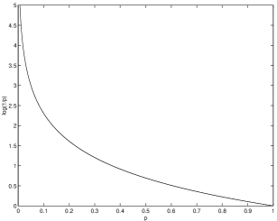
Figure 1.1: The unexpectedness of an event of probability $p$.

Intuitively we may justify calling $u$ the unexpectedness of the event $x$; this event is highly unexpected if it is almost sure not to happen, and has low unexpectedness if its probability is almost 1. The information in the random variable $X$ is thus the “eerily self-referential” [8] expectation value of $X$’s unexpectedness.

Shannon [9] formalised the requirements for an information measure $H(p_{1},\ldots,p_{n})$ with the following criteria:

1. $H$ should be continuous in the $p_{i}$.

2. If the $p_{i}$ are all equal, $p_{i}=1/n$, then $H$ should be a monotonic increasing function of $n$.

3. $H$ should be objective:

   $$H(p_{1},\ldots,p_{n})=H(p_{1}+p_{2},p_{3},\ldots,p_{n})+(p_{1}+p_{2})H\!\left(\frac{p_{1}}{p_{1}+p_{2}},\frac{p_{2}}{p_{1}+p_{2}}\right)$$ (1.11)

The last requirement here means that if we lump some of the outcomes together, and consider the information of the lumped probability distribution plus the weighted information contained in the individual “lumps”, we should have the same amount of information as in the original probability distribution. In the mathematical terminology of Aczél and Daróczy [10], the entropy is strongly additive. Shannon proved that the unique (up to an arbitrary factor) information measure satisfying these conditions is the entropy defined in Eqn 1.10. Several other authors, notably Rényi, and Aczél and Daróczy have proposed other criteria which uniquely specify Shannon entropy as a measure of information.

The arbitrary factor may be removed by choosing an appropriate logarithmic base. The most convenient bases are 2 and $e$, the unit of information in these cases being called the bit or the nat respectively; if in this discussion the base of the logarithm is significant it will be mentioned.

Some useful features to note about $H$ are:

• $H=0$ if and only if some $p_{i}=1$ and all others are zero; the information is zero only if we are certain of the outcome.

• If the probabilities are equalised, i.e. any two probabilities are changed to more equal values, then $H$ increases.

• If $p(a,b)=p_{A}(a)p_{B}(b)$ for all $a\in A,b\in B$ then

  $$H(A,B) = -\sum_{x\in A,y\in B}p(x,y)\log p_{A}(x)p_{B}(y)$$

  $$= -\sum_{x\in A,y\in B}p(x,y)\log p_{A}(x)-\sum_{x\in A,y\in B}p(x,y)\log p_{B}(y)$$

  $$= -\sum_{x\in A}p_{A}(x)\log p_{A}(x)-\sum_{y\in B}p_{B}(y)\log p_{B}(y)$$

  $$= H(A)+H(B)$$

We will be interested later in the information entropy of a more general distribution on a product sample space. So consider the information contained in the distribution $p(a,b)$ on random variables $X$ and $Y$, where $p$ is not a product distribution:

$$H(A,B) = -\sum_{x\in A,y\in B}p(x,y)\log p(x,y)$$ (1.12)

$$= -\sum_{x\in A,y\in B}p(x,y)\log p(y|x)p(x)$$

$$= -\sum_{x\in A,y\in B}p(x,y)\log p(y|x)-\sum_{x\in A}p_{A}(x)\log p_{A}(x)$$

$$= H(B|A)+H(A)$$

where we have defined the conditional entropy as

$$H(B|A)=-\sum_{x\in A,y\in B}p(x,y)\log p(y|x)=\sum_{x\in A}p(x)\sum_{y\in B}p(y|x)\log p(y|x).$$ (1.13)

Note that, for fixed $x\in A$, $p(y|x)$ is a probability distribution; so we could describe $H(Y|x)=\sum_{y\in B}p(y|x)\log p(y|x)$ as the $x$-based entropy. The conditional entropy is then the expectation value of the $x$-based entropy.

Using the concavity of the $\log$ function, it can be proved that $H(X,Y)\leq H(X)+H(Y)$: the entropy of a joint event is bounded by the sum of entropies of the individual events. Equality is achieved only if the distributions are independent, as shown above. From this inequality and Eqn 1.12 we find

$$H(Y|X)\leq H(Y)$$ (1.14)

with equality only if the distributions of $Y$ and $X$ are independent. In the case where they are not independent, learning about which value of $x$ was sampled from the set $A$ allows us to update our knowledge about what will be sampled from $B$, so our conditioned uncertainty (entropy) is less than the unconditioned. We could even extend our idea of conditioned information to many more than just two sample spaces; if we consider the random variables $X_{1},\ldots,X_{n}$ defined on spaces $A_{1},\ldots,A_{n}$, we can define

$$H(X_{n}|X_{n-1},\ldots,X_{1}) =-\sum_{x_{1}\ldots x_{n}} p(x_{1},\ldots,x_{n-1})\times$$

$$\sum_{x_{n}\in A_{n}}p(x_{n}|x_{1},\ldots,x_{n-1})\log p(x_{n}|x_{1},\ldots,x_{n-1})$$

to be the entropy of the next sampling given the sampled sequence once we know the preceding $n-1$ samples. By repeated application of the inequality above, we can show that

$$H(X_{n}|X_{n-1},\ldots,X_{1})\leq H(X_{n}|X_{n-1},\ldots,X_{2})\leq\ldots\leq H(X_{n}|X_{n-1})\leq H(X_{n}).$$ (1.15)

In general, conditioning reduces our entropy and uncertainty.

We will now employ the characterisation of an information source as a stochastic process as mentioned earlier. Consider a stationary stochastic source producing a sequence of random variables $X_{1},X_{2},\ldots$ and the “next-symbol” entropy $H(X_{n+1}|X_{n},\ldots,X_{1})$. Note that

$$H(X_{n+1}|X_{n},\ldots,X_{1}) \leq H(X_{n+1}|X_{n},\ldots,X_{2})$$

$$= H(X_{n}|X_{n-1},\ldots,X_{1})$$

where the equality follows from the stationarity of the process. Thus next-symbol entropy is a decreasing sequence of non-negative quantities and so has a limit. We call this limit the entropy rate of the stochastic process, $H(X)$. For a stationary stochastic process this is equal to the limit of the average entropy per symbol,

$$\frac{H(X_{1},\ldots,X_{n})}{n},$$ (1.16)

which is a further justification for calling this limit the unique entropy rate of the stochastic process.

Example 1.1.2.

Entropy rate of a binary channel Consider a stochastic source producing a random variable from the set $\{0,1\}$, with $p(0)=p,p(1)=1-p$. Then the entropy is a function of the real number $p$, given by $H(p)=-p\log p-(1-p)\log(1-p)$. This function is plotted in Figure 1.2.

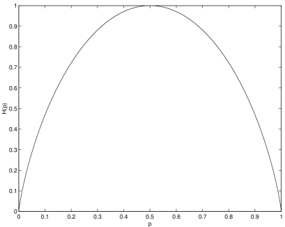
Figure 1.2: The entropy of a binary random variable.

Notice that the function is concave and achieves its maximum value of unity when $p=1/2$.

It was mentioned previously that entropy is a measure of our ignorance, and since we interpret probabilities as subjective belief in a proposition this “ignorance” must also be subjective. The following example, due to Uffink and quoted in [6], illustrates this. Suppose my key is in my pocket with probability 0.9 and if it is not there it could equally likely be in a hundred other places, each with probability $0.001$. The entropy is then $-0.9\log 0.9-100(0.001\log 0.001)=0.7856$. If I put my hand in my pocket and the key is not there, the entropy jumps to $-\log 0.01=4.605$: I am now extremely uncertain where it is! However, after checking my pocket there will on average be less uncertainty; in fact the weighted average is $-0.9\log 1-0.1\log 0.01=0.4605$.

1.1.3 Data Compression: Shannon’s Noiseless Coding Theorem

What is the use of the “entropy rate” of a stochastic source? If our approach to information is to be pragmatic, as mentioned previously, then we need to find a useful interpretation of this quantity.

We will first consider a stochastic source which produces independent, identically-distributed random variables $X_{1},X_{2},\ldots,X_{n}$. A typical sequence drawn from this source might be $x_{1}x_{2}\ldots x_{n}$ with probability $p(x_{1},\ldots,x_{n})=p(x_{1})\ldots p(x_{n})$. Taking logarithms of both sides and dividing by $n$, we find

$$\frac{1}{n}\log p(x_{1},\ldots,x_{n})=\frac{1}{n}\sum\log p(x_{i})$$ (1.17)

and by the law of large numbers the quantity on the right approaches the expectation value of the random variable $\log p(X)$, which is just the entropy $H(X)$. More precisely, if we consider the set

$$A_{\epsilon}^{(n)}=\{(x_{1},\ldots,x_{n})\in A|2^{-n(H(X)+\epsilon)}\leq p(x_{1},\ldots,x_{n})\leq 2^{-n(H(X)-\epsilon)}\}$$ (1.18)

then the following statements are consequences of the law of large numbers:

1. $\mbox{Prob}(A_{\epsilon}^{(n)})>1-\epsilon$ for $n$ sufficiently large.

2. $|A_{\epsilon}^{(n)}|>(1-\epsilon)2^{n(H(X)-\epsilon)}$ for $n$ sufficiently large, and $|\cdot|$ denotes the number of elements in the set.

3. $|A_{\epsilon}^{(n)}|<2^{n(H(X)+\epsilon)}$.

Thus we can find a set of roughly $2^{nH(X)}$ strings (out of a possible $|A|^{n}$, where $A$ is the set of possible symbols) which all have approximately the same probability, and the probability of producing a string not in the set is arbitrarily small.

The practical importance of this is evident once we associate, with each string in this “most-likely” set, a unique string from the set $\{0,1\}^{nH(X)}$. We thus have a code for representing strings produced by the stochastic source $\{X_{i}\}$ which makes arbitrarily small errors, and which uses $nH(X)$ binary digits to represent $n$ source symbols. We thus have the extremely useful interpretation of $H(X)$ as the expected number of bits required to represent long strings from the stochastic source producing random variables $\{X_{i}\}$, in the case where each random variable in the set is independently distributed.

We have not quite done all we claimed in the previous paragraph, since we have ignored the possibility of a more compact coding strategy. Let the strings from $A^{n}$ be arranged in order of decreasing probability, and let $N(q)$ be the number of strings, taken in this order, required to form a set of total probability $q$. Then Shannon proved the remarkable result that for $q\neq 0,1$

$$\lim_{n\rightarrow\infty}\frac{\log N(q)}{n}=H.$$ (1.19)

For large $n$ it makes no difference how we define “probable”: all probable sets contain about $2^{nH}$ elements!

Note also that if our strings are produced by an independent binary source with $p(0)\neq 1/2$ then $H(p)<1$ (see Ex 1.1.2). Thus our code strings are shorter than the source strings — we have compressed the information. The resulting code strings will have $p(0)\approx p(1)\approx 1/2$ and entropy rate close to unity.

We will now look at what changes when a fully stochastic source is considered. Instead of the random variables $X_{1},\ldots,X_{n}$ being independent, they are described by a probability distribution $p(x_{1},\ldots,x_{n})$. From the considerations above, we can design a code with string lengths $l(x_{1}\ldots x_{n})$ such that the expected length per symbol $L=\frac{1}{n}\sum p(x_{1},\ldots,x_{n})l(x_{1}\ldots x_{n})$ satisfies

$$\left|\frac{H(X_{1},\ldots,X_{n})}{n}-L\right|<\epsilon.$$ (1.20)

If our stochastic source is stationary, then $H(X_{1},\ldots,X_{n})/n$ approaches the entropy rate $H(X)$. Thus in this case too, the entropy rate describes the shortest code available for a particular source. A provably optimal — that is, shortest — code can be found using an algorithm discovered by Huffman [8], and the communication theorist now has an enormous variety of codes to choose from to suit his application.

For reference, Shannon’s first theorem in full generality is given below.

Theorem 1.

Shannon I Let ${\cal C}:A^{n}\rightarrow B$ be a code with binary codewords, and suppose ${\cal C}$ has the property that no code word is the prefix of another code word. For each ${\bf x}\in A^{n}$ we denote the length of the codeword ${\cal C}({\bf x})$ by $l_{\cal C}({\bf x})$ and define $L_{\cal C}=\frac{1}{n}\sum p({\bf x})l_{\cal C}({\bf x})$, the expected code word length per source symbol. Suppose the source is stochastic. Then there exists a code ${\cal C}$ such that

$$\frac{H(X_{1},\ldots,X_{n})}{n}\leq L_{\cal C}\leq\frac{H(X_{1},\ldots,X_{n})}{n}+\frac{1}{n}.$$ (1.21)

An arbitrarily small error rate can be achieved if and only if the first inequality is satisfied.

We can also use Shannon’s theorem to interpret the conditional entropy

$$H(X|Y)=H(X,Y)-H(Y).$$ (1.22)

The right-hand side of this equation may be viewed as the number of bits required to code $X$ and $Y$ together, less the number of bits required to specify $Y$ alone. The difference must surely be the average number of bits required to code $X$ once $Y$ is known - one could perhaps envisage using a different code for each random variable $Y$ already in our possession. This interpretation will be important for considerations in the next section.

1.1.4 Information Channels and Mutual Information

Suppose we have a microphone on a stage, and the President is speaking into it. The microphone will be hooked up to a loudspeaker system so that the assembled throng will be able to hear him. The President in this situation is an information source, stochastically producing words (or more generally sounds) near the microphone. Considered entirely separately, the loudspeaker is also a stochastic information source. If the technical crew have done their job there should not only be a correlation between the output of the loudspeaker, there should be a one-to-one correspondence. Another way of saying this is that if we know the sounds produced by the President, we should be absolutely certain of what sounds will be produced by the loudspeaker. A mathematical way of expressing this is

$$H(\mbox{loudspeaker}|\mbox{President})=0:$$ (1.23)

the uncertainty (entropy) once we know the President’s words should be zero. Of course a real microphone-amplifier-loudspeaker (MAL) system does introduce some errors, so in general the conditional entropy above may be some small positive amount. A measure of the fidelity of the MAL system could then be the reduction in entropy once we know the original information:

$$I(\mbox{loudspeaker}:\mbox{President})=H(\mbox{loudspeaker})-H(\mbox{loudspeaker}|\mbox{President}).$$ (1.24)

If somebody accidentally unplugged the microphone from the amplifier, then there would be no correlation between the President’s speech and the sound produced by the loudspeaker and these could be considered to be independent sources, in which case $H(\mbox{loudspeaker}|\mbox{President})=H(\mbox{loudspeaker})$ and

$$I(\mbox{loudspeaker}:\mbox{President})=0.$$ (1.25)

The quantity defined in Eqn 1.24 is called the mutual information between the President and the loudspeaker. In a general setting we would have two stochastic sources $X$ and $Y$ with a given joint distribution $p(x,y)$ (which could in fact be a distribution over n-tuples of symbols from $X$ and $Y$). The mutual information would then be

$$I(X:Y) = H(X)-H(X|Y)$$

$$= H(X)-H(X,Y)+H(Y)$$

$$= H(Y)-H(Y|X)$$ (1.27)

where we have used Eqn 1.12 to obtain the second equality. In this context, $H(X|Y)$ is sometimes referred to as the equivocation of the channel.

Before continuing to the application and interpretation of the mutual information, we note a few mathematical features of this function. We note first the pleasing symmetry $I(X:Y)=I(Y:X)$; the amount of information we gain about $X$ when we learn $Y$ is the same as the amount of information gained about $Y$ on learning $X$. Notice that, because $0\leq H(X|Y)\leq H(X)$, the mutual information is always non-negative and always less than the entropies $H(X)$ and $H(Y)$; the mutual information is zero if and only if the distributions on $X$ and $Y$ are independent. Finally observe that $H(X|X)=0$, whence $I(X:X)=H(X)$ — the self-information of a source is equal to its information entropy.

The mutual information is in fact a special case of another function, the relative information (otherwise known as Kullback-Leibler distance) between two distributions, which we mention here for completeness. The relative information between two probability distributions $p(x)$ and $q(x)$ is defined to be

$$D(p||q) = \sum_{x\in X}p(x)\log\frac{p(x)}{q(x)}$$

$$= E_{p}\log\frac{p(x)}{q(x)}.$$

Note that the relative information is not symmetric in $p$ and $q$. In fact $D$ has several very useful interpretations, notably as the expected number of bits over and above the $H(p)$ required by Shannon’s theorem if the code you are using is optimised for the non-occurring distribution $q$. It is also easy to see that the probability of observing a string $x_{1}x_{2}\ldots x_{n}$ from a source producing independent, identically-distributed symbols with distribution $p(x_{i})$ is related to the distance between the observed distribution and the real distribution. If we let $q(a_{i})=\frac{n_{i}}{n}$ be the empirical distribution drawn from the alphabet $\{a_{1},\ldots,a_{N}\}$ then

$$p(x_{1}x_{2}\ldots x_{n}) = \prod_{i=1}^{n}p(x_{i})=\prod_{j=1}^{N}p(a_{j})^{nq(a_{i})}$$

$$= \prod_{j=1}^{N}\exp[nq(a_{j})\log p(a_{j})]$$

$$= \exp\left(n\sum_{j=1}^{N}[q(a_{j})\log p(a_{j})-q(a_{j})\log q(a_{j})+q(a_{j})\log q(a_{j})]\right)$$

$$= \exp\left(-n[H(q)+D(q||p)]\right).$$

The mutual information is seen to be the relative information between the product distribution of $X$ and $Y$ and the true joint distribution:

$$I(X:Y) = \sum_{x\in X}\sum_{y\in Y}p(x,y)\log\frac{p(x,y)}{p(x)p(y)}$$

$$= D(p(x,y)||p(x)p(y))$$

and so is a measure of the correlation between $X$ and $Y$, that is, the extent to which they differ from being independent.

As discussed in the previous section, the conditional entropy $H(X|Y)$ is a measure of the expected number of bits required to code $X$ once we know the value of $Y$; the mutual information thus quantifies the information about $X$ conveyed by $Y$ and vice-versa, and lends a more rigorous interpretation to the mutual information than the heuristic explanation above. It also leads us directly to the idea of an information channel.

We characterise an information channel by the mistakes it makes, and this knowledge is generally derived from an understanding of the physical system used to convey the information. For example in the MAL system described above, the response of the amplifier will be frequency dependent and perhaps have an upper and lower cutoff; the loudspeaker in turn will also have a characteristic response, all of which will lead to hissing, random noise, feedback and other such unwanted effects. If we assume that the alphabet under consideration is a sequence of phonemes spoken by the President (we could alternatively analyse the spectrum of his voice), then what his PR people will be interested in is the probability that a given phoneme is produced by the loudspeaker when the President utters another given phoneme. The intermediate steps don’t interest them; what they care about is $p(\mbox{lspk=``ch''}|\mbox{Pres=``sh''})=0.1$, because this substitution could be damaging.

More rigorously, an information channel is characterised by an input alphabet $X$, an output alphabet $Y$ and the transition probabilities $p(y|x)$ that describe the probability of the input symbol $x$ being turned into output symbol $y$. For a given probability distribution over the input symbols $X$, we can calculate the mutual information (per symbol) between the input and output — and if we further assume that the channel can accept $r$ input symbols per unit time, then we begin to see an interesting problem before us: What is the fastest rate at which information can be conveyed across this channel? And can we transmit information with arbitrarily few errors despite the introduction of probabilistic errors by the channel?

These questions will take us to the heart of classical information theory. But to jump the gun a bit: The answer to the second question is Yes, and transmission without errors can take place at the rate

$$C=\max_{p(x)}I(X:Y)$$ (1.30)

bits per symbol. This is surprising, since one would imagine that we could either transmit rapidly or transmit faithfully, but not both at the same time. That this is so is the content of Shannon’s Second Theorem, the Noisy Coding Theorem, which will be the subject of the next section.

The quantity defined in Eqn 1.30 is called the capacity of the channel. In most cases of interest this can not be calculated explicitly, but some examples serve to illustrate the idea of capacity.

Example 1.1.3.

Noiseless and useless channels If we have a noiseless binary channel, so that $p(0|0)=1$ and $p(1|1)=1$ then the maximum possible output entropy is 1 bit per symbol and this capacity is achieved if we simply ensure that the source probabilities are $p(0)=p(1)=1/2$. On the other hand, if all the transition probabilities are equal to $1/2$ then we can never hope to transmit any information.

Example 1.1.4.

Binary symmetric channel Suppose a channel transmitting binary signals has probability $p$ of flipping each bit, independently of other bits or of the particular value of this bit. By the symmetry of the errors, we observe that to maximise the mutual information we should set $p(0)=p(1)=1/2$, so that $H(\mbox{transmitted})=1$. If the channel output is a 1, then Bob knows $p(1|0)=p$ and $p(1|1)=1-p$, so he calculates

$$C=1-H(p)$$ (1.31)

where $H$ is the binary entropy function plotted in Figure 1.2.

Example 1.1.5.

Ternary channel [9] Suppose we have a channel with three symbols as depicted in Figure 1.3,

Figure 1.3: The action of an uncertain ternary channel.

where one symbol 0 is transmitted without error, and the other two symbols 1 and 2 are interchanged with probability $p$. By symmetry, the capacity-achieving input source should have $p(0)=P$, $p(1)=p(2)=Q$. The mutual information will then be

$$I=-P\log P-2Q\log Q-2Q\alpha$$ (1.32)

where $\alpha=H(p)=-p\log p-(1-p)\log(1-p)$ is the noise due to the channel. We incorporate the constraint $P+2Q=1$ with a Lagrange multiplier; we must maximise $U=-P\log P-2Q\log Q-2Q\alpha+\lambda(P+2Q)$, whence

$$\frac{\partial U}{\partial P}=-1-\log P+\lambda=0$$

$$\frac{\partial U}{\partial Q}=-2-2\log Q-2\alpha+2\lambda=0.$$

Eliminating $\lambda$ we find $\log P=\log Q+\alpha$ or $P=Qe^{\alpha}$. Thus

$$P=\frac{e^{\alpha}}{e^{\alpha}+2}\hskip 28.45274ptQ=\frac{1}{e^{\alpha}+2}\hskip 28.45274ptC=\log\frac{e^{\alpha}+2}{e^{\alpha}}.$$ (1.33)

The channels we have considered here are described as memoryless. For the brave-hearted and strong-willed out there, one can also consider sources with memory i.e. where the error process can be considered as a stochastic process depending on arbitrarily many previous input and output symbols. Memoryless channels are, fortunately, the rule in situations of interest; and most examples of stochastic noise can be approximated by memoryless channels transmitting large symbol blocks.

1.1.5 Channel Capacity: Shannon’s Noisy Coding Theorem

The fundamental idea Shannon employed in showing that information can be transmitted reliably over a noisy channel was to allow a small probability of error, which goes to zero in some limit — in particular, in the limit when we code large blocks of symbols.

Figure 1.4 is a sketch of the communication system

Figure 1.4: Sketch of a communication system.

considered here. The stochastic source produces symbols (represented by the random variable $X$) drawn from the alphabet $A$, and a source encoder optimally codes strings of source symbols into strings of channel symbols drawn from the set $B$; this “combined source” is represented by $X_{s}$. The channel encoder introduces some redundancy into the message by mapping $m$ channel symbols into $r$ channel symbols, with $r>m$; this gives an effective source $X_{c}$. The output $Y_{c}$ of the channel is not necessarily a string in the range of the code $C$, and we use a decoding function $f$ to correct these changes. Finally a source decoder is applied; an error occurs whenever the random variable $X\neq Y$. With an optimal source encoder, we have $H(X_{s})=\log|B|$ — no redundancy — and $H(X)=\frac{m}{n}\log|B|$, where $|B|$ denotes the number of elements in B. The input to the channel then has entropy $H(X_{c})=\frac{m}{r}H(X_{s})$. The rate of the channel is defined to be $R=H(X_{c})$, that is, the number of useful bits conveyed per symbol sent. The channel capacity $C$ in this case is defined to be the mutual information of the channel symbols, $X_{s}$ and $Y_{c}$, maximised over all codes,

$$C=\max\{I(X_{s}:Y_{c})|C:B^{m}\rightarrow B^{r}\},$$ (1.34)

since the code will imply a probability distribution over the output symbols.

We are now ready to state Shannon’s Noisy Channel Coding Theorem.

Theorem 2.

Shannon II If $R\leq C$, there exists a code $C:B^{m}\rightarrow B^{r}$ such that the probability of a decoding error for any message (string from $B^{m}$) is arbitrarily small. Conversely, if the probability of error is arbitrarily small for a given code, then $R\leq C$.

Before we sketch a proof of this, we return to the idea of conditional entropy between the sent and received messages, $H(X_{c}|Y_{c})$. Suppose we have received an output $y_{1}\ldots y_{N}$; then if we had a noiseless side channel which could convey the “missing” information $NH(X_{c}|Y_{c})$, we could perfectly reconstruct the sent message. This means that there were on average $2^{NH(X_{c}|Y_{c})}$ errors which this side channel would allow us to correct, or equivalently that the received string, on average, could have originated from one of $2^{NH(X_{c}|Y_{c})}$ possible input strings. And this last fact is crucial to coding, since the optimal code will produce codewords which aren’t likely to diffuse to the same output string.

We begin by looking at the first statement in the theorem above. The strategy used by Shannon was to consider random codes (i.e. random one-to-one functions from the messages $B^{m}$ to the code words $B^{r}$) and average the probability of error over all these codes. The decoding technique will be to determine, for the received string $y_{1}\ldots y_{r}$, the set of $2^{r(H(X_{c}|Y_{c})+\delta)}$ most likely inputs, which we will call the decoding sphere $D_{\delta}$. We then decode this received string by associating it with a code word in its decoding sphere. Suppose without loss of generality that the input code word was $x^{(1)}$; then there are two cases in which an error could occur:

1. $x^{(1)}$ may not be in the decoding sphere;

2. There may be other code words apart from $x^{(1)}$ in the decoding sphere.

Given arbitrary $\epsilon>0$ and $\delta>0$, the probability that $x^{(1)}\in D_{\delta}$ can be made greater than $1-\epsilon$ by choosing $r$ large. So the probability of an error is

$$P_{e}\leq\epsilon+p\left(\mbox{$x^{(i)}\in D_{\delta}$ for at least one $i=2,3,\ldots,|B|^{m}$}\right).$$ (1.35)

There are $2^{rR}$ code words distributed among $|B|^{r}=2^{rH(X_{s})}$ strings from $B^{r}$; by the assumption of random coding, the probability that an arbitrary string is a code word is

$$p(\mbox{$X$ is a codeword})=\frac{2^{rR}}{2^{rH(X_{s})}}=2^{-r(H(X_{s})-R)}$$ (1.36)

independently of other code word assignments. We can now calculate the probability that $D_{\delta}$ contains a code word (apart from $x^{(1)}$):

$$p\left(\mbox{code word in $D_{\delta}$}\right) = \sum_{X\in D_{\delta},X\neq x^{(1)}}p(\mbox{$X$ is a codeword})$$ (1.37)

$$= \left(|D_{\delta}|-1\right)2^{-r(H(X_{s})-R)}=2^{-r\left(H(X_{s})-R-H(X_{c}|Y_{c})-\delta\right)}.$$

Now $H(X_{c}|Y_{c})=H(X_{s},X_{c}|Y_{c})=H(X_{c}|X_{s},Y_{c})+H(X_{s}|Y_{c})=H(X_{s}|Y_{c})$, where the first equality follows from the functional dependence of messages $X_{s}$ on code words $X_{c}$, the second follows from Eqn 1.12, and the third follows from the functional dependence of $X_{c}$ on $X_{s}$. Thus we can simplify the expression above:

$$p\left(\mbox{code word in $D_{\delta}$}\right)=2^{-r(I(X_{s}:Y_{c})-R-\delta)}$$ (1.38)

and we conclude that the probability of an error goes to zero exponentially (for large $r$) as long as $I(X_{s}:Y_{c})-\delta>R$. If we in fact employ the code that achieves channel capacity and choose $\delta$ to be arbitrarily small, then the condition for vanishing probability of error becomes

$$C\geq R$$ (1.39)

as desired.

Note that we have shown that the average probability of error can be made arbitrarily small:

$$\frac{1}{2^{rR}}\sum_{i}^{2^{r}R}p(\mbox{error when code word $x^{(i)}$ is sent})<\epsilon$$ (1.40)

Let the number of code words for which the probability of error is greater than $2\epsilon$ be denoted $N_{2\epsilon}$; then

$$\frac{1}{2^{rR}}N_{2\epsilon}(2\epsilon)<\epsilon$$ (1.41)

so that $N_{2\epsilon}<2^{rR-1}$. If we throw away these $N_{2\epsilon}$ code words and their messages then all code words have probability of error less than $2\epsilon$. There will now be $2^{rR-1}$ messages communicated, and the effective rate will be

Rate $$= \frac{\log(\mbox{number of messages})}{\mbox{number of symbols sent}}$$ (1.42)

$$= \frac{rR-1}{r}\rightarrow R$$

for large $r$.

For the converse, we begin by noting that the channel transition probability for a string of $r$ symbols factorises (by the memoryless channel assumption): $p(y_{1}\ldots y_{r}|x_{1}\ldots x_{r})=p(y_{1}|x_{1})\ldots p(y_{r}|x_{r})$. It is then easy to show that

$$H(Y_{c}^{r}|X_{s}^{r})=\sum_{i=1}^{r}H(Y_{c,i}|X_{s,i}).$$ (1.43)

Also, since $H(X,Y)\leq H(X)+H(Y)$, we have $H(Y_{c}^{r})\leq\sum_{i}H(Y_{c,i})$, so that

$$I(Y_{c}^{r}:X_{s}^{r}) = H(Y_{c}^{r})-H(Y_{c}^{r}|X_{s}^{r})$$

$$\leq \sum_{i=1}^{r}H(Y_{c,i}|X_{s,i})-H(Y_{c,i})$$

$$= \sum I(Y_{c,i}:X_{s,i})\leq rC.$$

But mutual information is symmetric, $I(X:Y)=I(Y:X)$, and using the fact that $H(X_{s}^{r})=rR$ we find

$$I(X_{s}^{r}:Y_{c}^{r})=H(X_{s}^{r})-H(X_{s}^{r}|Y_{c}^{r})=rR-H(X_{s}^{r}|Y_{c}^{r})\leq rC.$$ (1.44)

The quantity $\frac{1}{r}H(X_{s}^{r}|Y_{c}^{r})$ measures our average uncertainty about the input after receiving the channel output. If our error probability goes to zero as $r$ increases, then this quantity must become arbitrarily small, whence $R\leq C$.

1.2 Quantum Mechanics

Quantum mechanics is a theory that caught its inventors by surprise. The main reason for this is that the theory is heavily empirical and pragmatic in flavour — the formalism was forced onto us by experimental evidence — and so contradicted the principle-based “natural philosophy” tradition which had reaped such success in physics. In the absence of over-arching principles we are left with a formalism, fantastically successful, which is mute on several important subjects.

What is a quantum system? In the pragmatic spirit of the theory, a quantum system is one which cannot be described by classical mechanics. In general quantum effects become important when small energy differences become important, but in the absence of a priori principles we can give no strict definition. For example, NMR quantum computing can be described in entirely classical terms [11] and yet is advertised as the first demonstration of fully quantum computing; and Kitaev [12] has conjectured that some types of quantum systems can be efficiently simulated by classical systems. The quantum-classical distinction is not crucial to this thesis, where we are dealing with part of the formal apparatus of the theory; indeed, there is some hope that from this apparatus can be coaxed some principles to rule the quantum world [13].

For our purposes, the following axioms serve to define quantum mechanics:

1. States. A state of a quantum system is represented by a bounded linear operator $\rho$ (called a density operator) on a Hilbert space ${\cal H}$ satisfying the following conditions:

   • $\rho$ is Hermitian.

   • The sum of the eigenvalues is one, $\mbox{Tr}\;\rho=1$.

   • Every eigenvalue of $\rho$ is nonnegative, which we denote by $\rho\geq 0$.

   Vectors of the Hilbert space will be denoted by $|\psi\rangle$ (Dirac’s notation), and the inner product of two vectors is denoted $\langle\psi|\phi\rangle$. In all cases considered in this thesis, the underlying Hilbert space will be of finite dimension.

2. Measurement. Repeatable, or von Neumann, measurements are represented by complete sets of projectors $\Pi_{i}$ onto orthogonal subspaces of ${\cal H}$. By complete we mean that $\sum_{i}\Pi_{i}=\leavevmode\hbox{\small 1\kern-3.8pt\normalsize 1}$ (the identity operator), but the projectors are not required to be one-dimensional. Then the probability of outcome $i$ is

   $$p(i)=\mbox{Tr}\;\Pi_{i}\rho.$$ (1.45)

   After the measurement the new state is given by $\rho_{i}^{\prime}=\Pi_{i}\rho\Pi_{i}/\mbox{Tr}\;\Pi_{i}\rho$ if we know that outcome $i$ was produced, and otherwise by $\rho^{\prime}=\sum_{i}\Pi_{i}\rho\Pi_{i}$ if we merely know a measurement was made.

3. Evolution. When the system concerned is sufficiently isolated from the environment and no measurements are being made, evolution of the density operator is unitary:

   $$\rho\longrightarrow U\rho U^{\dagger},$$ (1.46)

   where $U$ is unitary so that $U^{-1}=U^{\dagger}$. The dynamics of the system are governed by the Schrödinger equation. In this thesis we will not be concerned about the specific operator $U$ relevant for a certain situation since we will be more concerned with evolutions that are in principle possible. However, we observe that for a given system the unitary operator is given by $U=\exp(iHt)$, where $H$ is the Hamiltonian of the system and $t$ is the time.

These are the basic tools of the mathematical formalism of quantum mechanics. In the following sections we will consider systems which are not fully isolated from their environment and in which measurements occur occasionally. Our aim is to complete our toolkit by discovering what evolutions are in principle possible for a real quantum system within the framework of the axioms above.

1.2.1 States and Subsystems

A density operator $\rho$ which is a one-dimensional projector is called a pure state. In this case $\rho=|\psi\rangle\langle\psi|$ for some vector $|\psi\rangle$ in the Hilbert space ${\cal H}$, and we frequently call $|\psi\rangle$ the state of the system. Pure states occupy a special place in quantum theory because they describe states of maximal knowledge [6] — no further experiments on such a pure state will allow us to predict more of the system’s behaviour. There is in fact a strong sense in which mixed states (to be discussed below) involve less knowledge than pure states: Wootters [15] showed that if the average value of a dynamical variable of a system is known, the uncertainty in this observable decreases if we have the additional knowledge that the state is pure.

The density operators form a convex set, which means that for any $(0\leq\lambda\leq 1)$, a convex combination $\lambda\rho_{1}+(1-\lambda)\rho_{2}$ of two density operators $\rho_{1},\rho_{2}$ is again a density operator. The pure states are also special in this context: they form the extreme points of this convex set, which means that there is no non-trivial way of writing a pure state $|\psi\rangle\langle\psi|$ as a convex combination of other density operators. Also, since a general density operator is Hermitian and positive, there exists a set $\{|\psi_{i}\rangle\}$ of vectors and real numbers $\lambda_{i}$ such that

$$\rho=\sum_{i=1}^{D}\lambda_{i}|\psi_{i}\rangle\langle\psi_{i}|$$ (1.47)

where $D$ is the dimension of the underlying Hilbert space; this result is the spectral theorem for Hemitian operators. The eigenvalues of $\rho$ are then the $\lambda_{i}$, and they sum to one. For this reason mixed states are frequently regarded as classical probability mixtures of pure states. Indeed, if we consider the ensemble in which the pure state $|\psi_{i}\rangle$ occurs with probability $\lambda_{i}$, and we make a measurement represented by the projectors $\{\Pi_{\nu}\}$, then the probability of the outcome $\mu$ is

$$p(\Pi_{\mu})=\sum_{i=1}^{D}\lambda_{i}\mbox{Tr}\;|\psi_{i}\rangle\langle\psi_{i}|\Pi_{\mu}=\mbox{Tr}\;\left(\sum_{i=1}^{D}\lambda_{i}|\psi_{i}\rangle\langle\psi_{i}|\Pi_{\mu}\right)=\mbox{Tr}\;\rho\Pi_{\mu}$$ (1.48)

where we have used the linearity of the trace to take the $\lambda$s inside.

Thus if a pure state results from maximal knowledge of a physical system, then a mixed state arises when our available knowledge of the system doesn’t uniquely identify a pure state — we have less than maximal knowledge. Mixed states arise in two closely related ways:

• We do not have as much knowledge as we could in principle, perhaps due to imperfections in our preparation apparatus, and must therefore characterise the state using a probability distribution over all pure states compatible with the knowledge available to us.

• The system $A$ is part of a larger system $AB$ which is in a pure state. In this case our knowledge of the whole system is maximal, but correlations between subsystems don’t permit us to make definite statements about subsystem $A$.

From an experimenter’s viewpoint these situations are indistinguishable. Consider the simplest canonical example of a quantum system, a two-level system which we will refer to as a qubit. We can arbitrarily label the pure states of the system $|0\rangle$ and $|1\rangle$, which could correspond to the two distinct states of the spin degree of freedom (‘up’ and ‘down’) in a spin-1/2 particle. The experimenter may produce these particles in an ionisation chamber, and the density matrix describing these randomly produced particles would be $\frac{1}{2}|0\rangle\langle 0|+\frac{1}{2}|1\rangle\langle 1|=\frac{1}{2}\leavevmode\hbox{\small 1\kern-3.8pt\normalsize 1}$. If he were extremely skilled, however, the experimenter could observe the interactions which produced each electron and write down an enormous pure state vector for the system. When he traced out the many degrees of freedom not associated with the electron to which his apparatus is insensitive, he would again be left with the state $\frac{1}{2}\leavevmode\hbox{\small 1\kern-3.8pt\normalsize 1}$.

The “tracing out of degrees of freedom” is achieved in the formalism by performing a partial trace over the ignored system. Suppose we consider two subsytems $A$ and $B$ and let $|1_{a}\rangle$ (where $a=1,\ldots,D_{1}$) and $|2_{\alpha}\rangle$ (where $\alpha=1,\ldots,D_{2}$) be orthonormal bases over the two systems’ Hilbert spaces respectively. Then if $\rho^{AB}$ is a joint state of the system, the reduced density matrix $\rho^{A}$ of system $A$ is

$$\rho^{A}=\sum_{\alpha=1}^{D_{2}}\langle 2_{\alpha}|\rho^{AB}|2_{\alpha}\rangle\equiv\mbox{Tr}_{B}\;\rho$$ (1.49)

with a similar expression holding for subsystem $B$. We frequently use the matrix elements $\rho^{AB}_{a\alpha,b\beta}=\langle 1_{a}|\langle 2_{\alpha}|\rho^{AB}|2_{\beta}\rangle|1_{b}\rangle$ of $\rho^{AB}$ to represent the density operator of a system; in this notation, the operation of partial trace looks like

$$\rho^{A}_{ab}=\sum_{\nu=1}^{D_{2}}\rho^{AB}_{a\nu,b\nu}.$$ (1.50)

As a converse to this, one can also consider the purifications of a mixed state. Suppose our state $\rho$ is an operator on the Hilbert space $H_{A}$ with spectral decomposition $\rho=\sum_{i}\lambda_{i}|\psi_{i}\rangle\langle\psi_{i}|$. Then consider the following vector from the space $H_{A}\otimes H_{B}$ ($\dim H_{A}\leq\dim H_{B}$):

$$|\Psi^{AB}\rangle=\sum_{i}\sqrt{\lambda_{i}}|B_{i}\rangle\otimes|\psi_{i}\rangle,$$ (1.51)

with the $|B_{i}\rangle$ any orthogonal set in $H_{B}$. Then $\rho=\mbox{Tr}_{B}\;|\Psi^{AB}\rangle\langle\Psi^{AB}|$, so $\rho$ can be considered to be one part of a bipartite pure state. There are of course an infinite number of alternative purifications of a given mixed state.

Example 1.2.1.

Two spin-1/2 systems The simplest bipartite system is a system of two qubits. The sets $\{|0_{A}\rangle,|1_{A}\rangle\}$ and $\{|0_{B}\rangle,|1_{B}\rangle\}$ are bases for the two individual qubit’s spaces. If we denote a vector $|i_{A}\rangle\otimes|j_{B}\rangle$ by $|ij\rangle$, then a basis for the combined system is $\{|00\rangle,|01\rangle,|10\rangle,|11\rangle\}$. Consider the pure state of the combined system

$$|\psi^{-}\rangle=\frac{1}{\sqrt{2}}\left(|10\rangle-|01\rangle\right);$$ (1.52)

which has density matrix

$$\rho^{AB}=|\psi^{-}\rangle\langle\psi^{-}|=\frac{1}{2}\bigg{(}|10\rangle\langle 10|+|01\rangle\langle 01|-|10\rangle\langle 01|-|01\rangle\langle 10|\bigg{)};$$ (1.53)

tracing out system $B$ removes the second index and retains only those terms where the second index of the bra and ket are the same. So the reduced density matrix of system $A$ is $\rho^{A}=\frac{1}{2}(|1\rangle\langle 1|+|0\rangle\langle 0|)=\frac{1}{2}\leavevmode\hbox{\small 1\kern-3.8pt\normalsize 1}$.

The singlet state $|\psi^{-}\rangle$ is a state of maximum uncertainty in each subsystem. This is because of the high degree of entanglement between its two subsystems — and this state, along with the triplet states $|\psi^{+}\rangle$ and $|\phi^{\pm}\rangle$, is a canonical example of all the marvel and mystery behind quantum mechanics. We will return to investigate some properties of this state in later chapters.

1.2.2 Generalised Measurements

Von Neumann measurements turn out to be unnecessarily restrictive: the number of distinct outcomes is limited by the dimensionality of the system considered, and we can’t answer simple questions that have useful classical formulations [6, p. 280]. Our remedy for this is to adopt a new measurement technique. Suppose we wish to make a measurement on a quantum state $\rho^{s}$ with Hilbert space $H_{s}$. We will carry out the following steps:

• Attach an ancilla system in a known state $\rho^{a}$. The state of the combined system will be the product state $\rho^{s}\otimes\rho^{a}$. Note that our ancilla Hilbert space could have as many dimensions as we require.

• Evolve the combined system unitarily, $\rho^{s}\otimes\rho^{a}\longrightarrow U\rho^{s}\otimes\rho^{a}U^{\dagger}$. The resulting state is likely going to be entangled.

• Make a von Neumann measurement on just the ancilla represented by the projectors $\leavevmode\hbox{\small 1\kern-3.8pt\normalsize 1}_{s}\otimes\Pi_{\alpha}$, where $\Pi_{\alpha}$ acts on the ancilla. The probability of outcome $\alpha$ will then be

  $$p(\alpha)=\mbox{Tr}\;\left(\leavevmode\hbox{\small 1\kern-3.8pt\normalsize 1}\otimes\Pi_{\alpha}U\rho^{s}\otimes\rho^{a}U^{\dagger}\right).$$ (1.54)

Of course we are not interested in the (hypothetical) ancilla system we have introduced, and so we can simplify our formalism by tracing it out earlier. If we write

$$E_{\alpha}=\mbox{Tr}_{\mbox{\scriptsize ancilla}}\;\left(\leavevmode\hbox{\small 1\kern-3.8pt\normalsize 1}\otimes\Pi_{\alpha}U\leavevmode\hbox{\small 1\kern-3.8pt\normalsize 1}\otimes\rho^{a}U^{\dagger}\right)$$ (1.55)

then $E_{\alpha}$ is an operator over the system Hilbert space $H_{s}$, and the probability of outcome $\alpha$ is given by the much simpler formula $p(\alpha)=\mbox{Tr}\;(E_{\alpha}\rho^{s})$, where the trace is over just the system degrees of freedom. Note that the final two steps can be amalgamated: unitary evolution followed by measurement is exactly the same as a measurement in a different basis. However in this case we will have to allow a von Neumann measurement on the combined system, not just the ancilla.

The set of operators $\{E_{\alpha}\}$ is called a POVM, for Positive Operator-Valued Measure, and represents the most general type of measurement possible on a quantum system. Note that, in contrast with a von Neumann measurement, these operators are not orthogonal and at first glance there doesn’t appear to be any simple way to represent the state just after a measurement has been made. We will return to this in the next section.

The set $\{E_{\alpha}\}$ has the following characteristics:

1. $\sum_{\alpha}E_{\alpha}=\leavevmode\hbox{\small 1\kern-3.8pt\normalsize 1}$.

2. Each $E_{\alpha}$ is a Hermitian operator.

3. All the eigenvalues of the $E_{\alpha}$ are non-negative i.e. $E_{\alpha}\geq 0$.

These are in some sense the minimum specifications required to extract probabilities from a density operator. The first requirement ensures that the probability of obtaining some outcome is one; the second ensures that the probabilities are real numbers, and the third guarantees that these real numbers are non-negative. It is therefore pleasing that any set of operators satisfying these 3 conditions can be realised using the technique described at the start of this section: this is the content of Kraus’ Theorem [6]. So if we define a POVM by the above three requirements, we are guaranteed that this measurement can be realised by a repeatable measurement on a larger system. And the above characterisation is a lot easier to work with!

1.2.3 Evolution

What quantum state are we left with after we have performed a POVM on a given quantum state? We will first look at this question for the case where the system starts in a pure state, $\rho^{s}=|\psi^{s}\rangle\langle\psi^{s}|$, and the ancilla is in a mixed state $\rho^{a}=\sum_{i}\mu_{i}|\phi^{a}_{i}\rangle\langle\phi^{a}_{i}|$. Then according to the measurement axiom presented previously, the final state of the combined system will be

$$\rho^{sa}_{\alpha}=\frac{1}{\mbox{Tr}\;(E_{\alpha}\rho^{s})}\sum_{i}\mu_{i}UP_{\alpha}|\psi^{s}\rangle\otimes|\phi^{a}_{i}\rangle\langle\psi^{s}|\otimes\langle\phi^{a}_{i}|P_{\alpha}U^{\dagger}$$ (1.56)

where $P_{\alpha}=U^{\dagger}(\leavevmode\hbox{\small 1\kern-3.8pt\normalsize 1}\otimes\Pi_{\alpha})U$ represents a projection onto some combined basis of the system and ancilla. Now we define a set of operators on the system,

$$M_{(i,k)\alpha}=\sqrt{\mu_{i}}\>(\leavevmode\hbox{\small 1\kern-3.8pt\normalsize 1}\otimes\langle\xi_{k}|)P_{\alpha}(\leavevmode\hbox{\small 1\kern-3.8pt\normalsize 1}\otimes|\phi^{a}_{i}\rangle),$$ (1.57)

where $|\xi_{k}\rangle$ is an arbitrary orthonormal basis for the ancilla Hilbert space and $E_{\alpha}$ is the corresponding POVM element. Then the state of the system after measurement can be expressed in terms of these operators:

$$\rho^{s}_{\alpha} = \frac{1}{\mbox{Tr}\;(E_{\alpha}\rho^{s})}\mbox{Tr}_{\mbox{\scriptsize ancilla}}\;\bigg{(}\sum_{i}\mu_{i}P_{\alpha}|\psi^{s}\rangle\otimes|\phi^{a}_{i}\rangle\langle\psi^{s}|\otimes\langle\phi^{a}_{i}|P_{\alpha}\bigg{)}$$ (1.58)

$$= \frac{1}{\mbox{Tr}\;(E_{\alpha}\rho^{s})}\sum_{\bf b}M_{{\bf b}\alpha}|\psi^{s}\rangle\langle\psi^{s}|M_{{\bf b}\alpha}^{\dagger}$$

where we have amalgamated the indices $(i,k)$ into one index ${\bf b}$. This operation is linear so that for any mixed state $\rho^{s}$, the state after measurement is

$$\rho^{s}_{\alpha}=\frac{1}{\mbox{Tr}\;(E_{\alpha}\rho^{s})}\sum_{\bf b}M_{{\bf b}\alpha}\rho^{s}M_{{\bf b}\alpha}^{\dagger}$$ (1.59)

if we know that the outcome is $\alpha$, and

$$\rho^{s}=\sum_{\alpha}p(\alpha)\rho^{s}_{\alpha}=\sum_{{\bf b}\alpha}M_{{\bf b}\alpha}|\psi^{s}\rangle\langle\psi^{s}|M_{{\bf b}\alpha}^{\dagger}$$ (1.60)

if we only know that a measurement has been made. Note that we can choose different orthonormal bases $|\xi_{k}\rangle$ for each value of $\alpha$ to make the representation as simple as possible — and that in general, the state resulting from a POVM depends on exactly how the POVM was implemented. The operators $M_{{\bf b}\alpha}$ are not free, however; they must satisfy

$$\sum_{\bf b}M^{\dagger}_{{\bf b}\alpha}M_{{\bf b}\alpha} = \sum_{i,k}\mu_{i}(\leavevmode\hbox{\small 1\kern-3.8pt\normalsize 1}\otimes\langle\xi_{k}|)P_{\alpha}(\leavevmode\hbox{\small 1\kern-3.8pt\normalsize 1}\otimes|\phi^{a}_{i}\rangle)(\leavevmode\hbox{\small 1\kern-3.8pt\normalsize 1}\otimes\langle\phi^{a}_{i}|)P_{\alpha}(\leavevmode\hbox{\small 1\kern-3.8pt\normalsize 1}\otimes|\xi_{k}\rangle)$$ (1.61)

$$= \mbox{Tr}_{\mbox{\scriptsize ancilla}}\;\bigg{[}P_{\alpha}(\leavevmode\hbox{\small 1\kern-3.8pt\normalsize 1}\otimes\rho^{a})P_{\alpha}\bigg{]}$$

$$= \mbox{Tr}_{\mbox{\scriptsize ancilla}}\;\bigg{[}\leavevmode\hbox{\small 1\kern-3.8pt\normalsize 1}\otimes\Pi_{\alpha}U\leavevmode\hbox{\small 1\kern-3.8pt\normalsize 1}\otimes\rho^{a}U^{\dagger}\bigg{]}=E_{\alpha}$$

(from Eqn 1.55). We will call a generalised measurement efficient if for each value of $\alpha$, there is only one value of ${\bf b}$ in the sum in Eqn 1.59; such a measurement is called efficient because pure states are mapped to pure states, so if we have maximal knowledge of the system before the measurement this is not ruined by our actions.

Suppose now we have an arbitrary set of operators $N_{\mu}$ satisfying (as do the $M_{{\bf b}\alpha}$ above) $\sum_{\mu}N_{\mu}^{\dagger}N_{\mu}=\leavevmode\hbox{\small 1\kern-3.8pt\normalsize 1}$. Then the mapping defined by

$$\rho\longrightarrow\$(\rho)=\sum_{\mu}N_{\mu}\rho N_{\mu}^{\dagger}$$ (1.62)

is called an operator-sum and has the following convenient properties:

1. If $\mbox{Tr}\;\rho=1$ then $\mbox{Tr}\;\$(\rho)=1$ ($\$$ is trace-preserving).

2. $\$$ is linear on the space of bounded linear operators on a given Hilbert space.

3. If $\rho$ is Hermitian then so is $\$(\rho)$.

4. If $\rho\geq 0$ then $\$(\rho)\geq 0$ (we say $\$$ is positive).

If we add one more condition to this list, then this list defines an object called a superoperator. This extra condition is

1. Let $\leavevmode\hbox{\small 1\kern-3.8pt\normalsize 1}_{n}$ be the identity on the $n$-dimensional Hilbert space. We require that the mapping $T_{n}=\$\otimes\leavevmode\hbox{\small 1\kern-3.8pt\normalsize 1}_{n}$ be positive for all $n$. This is called complete positivity.

Physically, this means that if we include for consideration any extra system $X$ — perhaps some part of the environment — so that the combined system is possibly entangled, but the system $X$ evolves trivially (it doesn’t evolve), the resulting state should still be a valid density operator. It turns out that an operator-sum does satisfy this requirement and so any operator-sum is also a superoperator.

Superoperators occupy a special place in the hearts of quantum mechanicians precisely because they represent the most general possible mappings of valid density operators to valid density operators, and thus the most general allowed evolution of physical states. It is thus particularly pleasing that we have the following theorems (proved in [16]):

1. Every superoperator has an operator-sum representation.

2. Every superoperator can be physically realised as a unitary evolution of a larger system.

The first theorem is a technical one, giving us a concrete mathematical representation for the “general evolution” of an operator. The second theorem has physical content, and tells us that what we have plucked out of the air to be “the most general possible evolution” is consistent with the physical axioms presented previously.

Chapter 2 Information in Quantum Systems

At the start of the previous chapter, we identified information as an abstract quantity, useful in situations of uncertainty, which was in a particular sense independent of the symbols used to represent it. In one example we had the option of using symbols Y and N or integers $\{0,1,\ldots,365\}$. But we in fact have even more freedom than this: we could communicate an integer by sending a bowl with $n$ nuts in it or as an $n$ volt signal on a wire; we could relay Y or N as letters on a piece of paper or by sending Yevgeny instead of Nigel.

Physicists are accumstomed to finding, and exploiting, such invariances in nature. The term “Energy” represents what we have to give to water to heat it, or what a rollercoaster has at the top of a hump, or what an exotic particle possesses as it is ejected from a nuclear reaction. Information thus seems like a prime candidate for the attention of physicists, and the sort of questions we might ask are “Is information conserved in interactions?”, “What restrictions are there to the amount of information we can put into a physical system, and how much can we take out of one?” or “Does information have links to any other useful concepts in physics, like energy?”. This chapter addresses some of these questions.

The physical theory which we will use to investigate them is of course quantum mechanics. But — and this is another reason for studying quantum information theory — such considerations are also giving us a new perspective on quantum theory, which may in time lead to a set of principles from which this theory can be derived.

One of the major new perspectives presented by quantum information theory is the idea of analysing quantum theory from within. Often such analyses take the form of algorithms or cyclic processes, or in some circumstances even games [17]; in short, the situations considered are finite and completely specified. The aims of such investigations are generally:

• To discover situations (games, communication problems, computations) in which a system behaving quantum mechanically yields qualitatively different results from any similar system described classically.

• To investigate extremal cases of such “quantum violation” and perhaps deduce fundamental limits on information storage, transmission or retrieval. Such extremal principles could also be useful in uniquely characterising quantum mechanics.

• To identify and quantify the quantum resources (such as entanglement or superposition) required to achieve such qualitative differences, and investigate the general properties of these resources.

In many of these investigations, the co-operating parties Alice and Bob (and sometimes their conniving acquaintance Eve) are frequently evoked and this thesis will be no exception. In this chapter we consider a message to be sent from Alice to Bob, encoded in the quantum state of a system. For the moment we will be assuming that the quantum state passes unchanged (and in particular is not subject to degradation or environmental interaction) between them.

2.1 Physical Implementation of Communication

Figure 2.1: Alice and Bob using a physical system to convey information

In classical information theory, the bit is a primitive notion. It is an abstract unit of information corresponding to two alternatives, which are conveniently represented as 0 and 1. Some of the characteristics of information encoded in bits are that it can be freely observed and copied (without changing it), and that after observing it one has exactly the right amount of information to prepare a new instance of the same information. Also, in order to specify one among $N$ alternatives we require $\log N$ bits.

The quantum version of a two-state system has somewhat different properties. Typical examples of two state systems are spin-1/2 systems, where the ‘spin up’ state may be written $|\!\uparrow\rangle$ and ‘spin down’ $|\!\downarrow\rangle$, or the polarisation states of photons, which may be written $|\!\updownarrow\rangle$ for vertical polarisation and $|\!\leftrightarrow\rangle$ for horizontal. For convenience we will label these states $|0\rangle$ and $|1\rangle$, using the freedom of representation discussed previously. A new feature arises immediately in that the quantum two-state system — or qubit — can exist in the superposition state $|0\rangle+|1\rangle$ which, if measured in the conventional basis $\{|0\rangle,|1\rangle\}$ will yield a completely random outcome.

We will analyse the communication setup represented in Figure 2.1. Alice prepares a state of the physical system A and sends the system to Bob who is free to choose the measurement he makes on A. Bob is aware of the possible preparations available to Alice, but of course is uncertain of which one in particular was used. We will identify three different types of information in physical systems (preparation, missing and accessible information) and briefly contrast the quantum information content with the information of an equivalent classically described system.

2.1.1 Preparation Information

Let us suppose for a moment that Alice and Bob use only pure states of a quantum system to communicate (mixed states will be discussed later). To be more specific, suppose they are using a two-level system and the $k^{\rm th}$ message state is represented by

$$|\psi_{k}\rangle=a_{k}|0\rangle+b_{k}|1\rangle$$ (2.1)

where $a_{k}$ and $b_{k}$ are complex amplitudes. We can choose the overall phase so that $a_{k}\in\mbox{\Bbb R}$ in which case $|\psi_{k}\rangle$ is specified by two real numbers ($a_{k}$ and the phase of $b_{k}$). How much information in a real number? An infinite amount, unfortunately. We overcome this problem, as frequently done in statistical physics, by coarse-graining — in this case by giving the real number to a fixed number of decimal places. In practice, Alice’s preparation equipment will in any case have some finite resolution so she can only distinguish between a finite number ${\cal N}$ of signals. So to prepare a signal state of this qubit Alice must specify $\log{\cal N}$ bits of information — and if she wants Bob to have complete knowledge of which among the signal states was prepared, she must send him exactly $\log{\cal N}$ classical bits.

If Alice and Bob are using an $N$-level quantum system the state of the system is represented by a ray in a projective Hilbert space ${\cal H}$. A natural metric on ${\cal H}$, given by Wootters [19], is

$$d(\psi_{0},\psi_{1})=\cos^{-1}|\langle\psi_{0}|\psi_{1}\rangle|$$ (2.2)

where the $|\psi_{i}\rangle$ are normalised representatives of their equivalence classes. With this metric, the compact space ${\cal H}$ can be partitioned into a finite number ${\cal N}$ of cells each with volume less than a fixed resolution $d{\cal V}$, and these cells can be indexed by integers $j=1,2,\ldots,{\cal N}$. By making $d{\cal V}$ small enough, any ray in cell $j$ can be arbitrarily well approximated by a fixed pure state $|\psi_{j}\rangle$ which is inside cell $j$. Thus our signal states are the finite set $\{|\psi_{1}\rangle,\ldots,|\psi_{\cal N}\rangle\}$, and they occur with some pre-agreed probabilities $p_{1},\ldots,p_{\cal N}$.

At this point we can compare the quantum realisation of signal states with an equivalent classical situation. In the classical case, the system will be described by canonical co-ordinates $P_{1},\ldots,P_{F},Q_{1},\ldots,Q_{F}$ in a phase space. We can select some compact subset $W$ to represent practically realisable states, and partition $W$ into a finite number ${\cal N}$ of cells of phase space volume smaller than $d{\cal V}_{c}$. A typical state of the system corresponds to a point in the phase space, but on this level of description we associate any state in cell $j$ with some fixed point in that cell.

By “preparation information” we mean the amount of information, once we know the details of the coarse-graining discussed above, required to unambiguously specify one of the cells. From the discussion of information theory presented in Chapter 1, we know that the classical information required, on average, to describe a preparation is

$$H(p)=-\sum p(j)\log p(j)$$ (2.3)

which is bounded above by $\log{\cal N}$. Thus by making our resolution volume ($d{\cal V}$ or $d{\cal V}_{c}$) small enough, we can make the preparation information of the system as large as we want.

How small can we make it?

Von Neumann Entropy and Missing Information

In classical statistical mechanics, there is a state function which is identified as “missing information”. Given some incomplete information about the state of a complicated system (perhaps we know its temperature $T$, pressure $P$ and volume $V$), the thermodynamic entropy is defined, up to an additive constant, to be

$$S(T,V,P)=k\log W(T,V,P)$$ (2.4)

where $W$ is the statistical weight of states which have the prescribed values of $T$,$V$ and $P$; this is the Boltzmann definition of entropy. The idea is very similar to that expressed in Chapter 1: the function $S(T,V,P)$ is, loosely speaking, the number of extra bits of information required — once we know $T$,$V$ and $P$ — in order to determine the exact state of the system. According to the Bayesian view, these macroscopic variables are background information which allow us to assign a prior probability distribution; our communication setup is completely equivalent to this except for the fact that we prescribe the probability distribution ourselves. So it is reasonable to calculate a function similar to Eqn 2.4 for our probability distribution and call it “missing information”.

Consider an ensemble of $\nu\gg 1$ classical systems as described above. Since $\nu$ is large, the number $\nu_{j}$ of systems in this ensemble which occupy cell $j$ is approximately $p(j)\nu$. The statistical weight is then the number of different ensembles of $\nu$ systems which have the same number of systems in each cell [23]:

$$\frac{\nu!}{\nu_{1}!\ldots\nu_{\cal N}!}.$$ (2.5)

The information missing towards a “microstate” description of the classical state is the average information required to describe the ensemble:

$$S(p) = \frac{1}{\nu}k\log\frac{\nu!}{\nu_{1}!\ldots\nu_{\cal N}!}$$ (2.6)

$$= -k\sum p(j)\log p(j)$$

where we have used Stirling’s approximation. Thus, up to a factor which expresses entropy in thermodynamic units, the information missing towards a microstate description of a classical system is equal to the preparation information.

The von Neumann entropy of a quantum state $\rho$ is defined to be

$$S(\rho)=-\mbox{Tr}\;(\rho\log\rho).$$ (2.7)

While this definition shares many properties with classical thermodynamic entropy, the field of quantum information theory exists largely because of the differences between these functions. However, there are still strong reasons for associating von Neumann entropy with missing information. Firstly, if the ensemble used for communication is the eigenensemble of $\rho$ (i.e. the eigenvectors $|\phi_{i}\rangle$ of $\rho$ appearing with probabilities equal to the eigenvalues $\lambda_{i}$) then an orthogonal measurement in the eigenbasis of $\rho$ will tell us exactly which signal was sent. Secondly, if $S(\rho)>0$ then any measurement (orthogonal or a POVM) whose outcome probabilities $q_{k}=\mbox{Tr}\;(\rho E_{k})$ yield less information than $S(\rho)$ cannot leave the system in a pure quantum state [14]. Intuitively, we start off missing $S(\rho)$ bits of information to a maximal description of the system, and discovering less information than this is insufficient to place the system in a pure state.

Some properties of the von Neumann entropy are [22], [21]:

1. Pure states are the unique zeros of the entropy. The unique maxima are those states proportional to the unit matrix, and the maximum value is $\log D$ where $D$ is the dimension of the Hilbert space.

2. If $U$ is a unitary transformation, then $S(\rho)=S(U\rho U^{\dagger})$.

3. $S$ is concave i.e. if $\lambda_{1},\ldots,\lambda_{n}$ are positive numbers whose sum is 1, and $\rho_{1},\ldots,\rho_{n}$ are density operators, then

   $$S(\sum_{i=1}^{n}\lambda_{i}\rho_{i})\geq\sum_{i=1}^{n}\lambda_{i}S(\rho_{i}).$$ (2.8)

   Intuitively, this means that our missing knowledge must increase if we throw in additional uncertainties, represented by the $\lambda_{i}$’s.

4. $S$ is additive, so that if $\rho_{A}$ is a state of system $A$ and $\rho_{B}$ a state of system $B$, then $S(\rho_{A}\otimes\rho_{B})=S(\rho_{A})+S(\rho_{B})$. If $\rho_{AB}$ is some (possibly entangled) state of the systems, and $\rho_{A}$ and $\rho_{B}$ are the reduced density matrices of the two subsystems, then

   $$S(\rho_{AB})\leq S(\rho_{A})+S(\rho_{B}).$$ (2.9)

   This property is known as subadditivity, and means that there can be more predictability in the whole than in the sum of the parts.

5. Von Neumann entropy is strongly subadditive, which means that for a tripartite system in the state $\rho_{ABC}$,

   $$S(\rho_{ABC})+S(\rho_{B})\leq S(\rho_{AB})+S(\rho_{BC}).$$ (2.10)

   This technical property, which is difficult to prove (see [21]), reduces to subadditivity in the case where system $B$ is one-dimensional.

So what is the relationship between preparation information and missing information in the quantum mechanical version of the communication system? Well, given the background information discussed above (i.e. knowledge of the coarse-grained cells and their a priori probabilities) but no preparation information (we don’t know which coarse-grained cell was chosen), the density operator we assign to the system is $\rho=\sum p(j)|\psi_{j}\rangle\langle\psi_{j}|$; so the missing information is $S(\rho)$. Now it can be shown [21] that

$$S(\rho)=-\sum_{k=1}^{D}\lambda_{k}\log\lambda_{k}\leq-\sum_{j=1}^{\cal N}p(j)\log p(j)=I_{P}.$$ (2.11)

In this expression, the $\lambda_{k}$ are eigenvalues of $\rho$, $D$ is the dimension of $\rho$, and $I_{P}$ is the preparation information for the ensemble. Equality holds if and only if the ensemble is the eigenensemble of $\rho$, that is, if all the signal states are orthogonal.

The conclusion is that preparation information $I_{P}$ and missing information $S$ are equal in classical physics, but in quantum physics $S\leq I_{P}$, and the preparation information can be made arbitrarily large. One question still remains: How much information can be extracted from the quantum state that Alice has prepared?

2.1.2 Accessible Information

Alice and Bob share the “background” information concerning the partitioning of the projective Hilbert space and the probability distribution of signals $p(j)$. Bob, knowing this information and no more, will ascribe a mixed state $\rho=\sum_{i}p(i)|\psi_{i}\rangle\langle\psi_{i}|$to the system he receives. His duty in the communication scenario is to determine as well as he can which pure state he received. Of course, if he has very precise measuring equipment which enables him to perform von Neumann (orthogonal) measurements, he can say immediately after the measurement that the system is in a pure state — if the measurement outcome was ‘3’, he knows the system is now exactly in state $|3\rangle$. But this information is not terribly useful for communication.

Unfortunately for Bob, exact recognition of unknown quantum states is not possible. This is related to the fact that there is no universal quantum cloning machine [35]; that is, there doesn’t exist a superoperator $\$$ which acts on an arbitrary state $|\psi\rangle$ and an ancilla in standard state $|s\rangle$ as

$$\$:|\psi\rangle|s\rangle\longrightarrow|\psi\rangle|\psi\rangle.$$ (2.12)

Cloning violates either the unitarity or the linearity of quantum mechanics (see Section 2.2), and could be used for instantaneous signalling [36] or discrimination between non-orthogonal quantum states.

The only option open to Bob, once he receives the quantum system from Alice, is to perform a POVM on the system. Suppose Bob chooses to perform the POVM $\{E_{b}\}$; the probability of outcome $b$ is $\mbox{Tr}\;(\rho E_{b})$. His task is to infer which state was sent, and so he uses Bayes’ Theorem (Eqn 1.8):

$$p({\rm P}_{j}|{\rm O}_{b})=\frac{p({\rm O}_{b}|{\rm P}_{j})p({\rm P}_{j})}{p({\rm O}_{b})}$$ (2.13)

where ${\rm O}_{b}$ represents the event “The outcome is $b$” and ${\rm P}_{j}$ the event “The preparation was in cell $j$”. We can calculate all the quantities on the right side of this expression: $p({\rm O}_{b})=\mbox{Tr}\;\rho E_{b}$, $p({\rm O}_{b}|{\rm P}_{j})=\mbox{Tr}\;|\psi_{j}\rangle\langle\psi_{j}|E_{b}=\langle\psi_{j}|E_{b}|\psi_{j}\rangle$ and $p({\rm P}_{j})=p(j)$. Thus we can calculate the post-measurement entropy

$$H({\rm P}|{\rm O})=-\sum_{b}p({\rm O}_{b})\sum_{j}p({\rm P}_{j}|{\rm O}_{b})\log p({\rm P}_{j}|{\rm O}_{b}).$$ (2.14)

We can now define the information gain due to the measurement $\{E_{b}\}$ as

$$I(\{E_{b}\})=I_{P}-H({\rm P}|{\rm O})$$ (2.15)

and the accessible information [24] is defined as

$$J=\max_{\{E_{b}\}}I(\{E_{b}\}).$$ (2.16)

The accessible information is the crucial characteristic of a physical communication system. In classical physics, states in different phase space cells are perfectly distinguishable as long as Bob’s measuring apparatus has fine enough resolution; hence the accessible information is in principle equal to the preparation information and the missing information. What can be said in the quantum situation?

The accessible information is unfortunately very difficult to calculate, as is the measurement which realises the maximum in Eqn 2.16. Davies [25] has shown that the optimal measurement consists of unnormalised projectors $E_{1},\ldots,E_{N}$, where the number of such projectors is bounded by $D\leq N\leq D^{2}$, where $D$ is the Hilbert space dimension. Several upper and lower bounds have been derived [26], some of which yield measurements that attain the bound. The most well-known bound is the Holevo Bound, first proved by Holevo in 1973 [27]. The bound is

$$J\leq S(\rho);$$ (2.17)

accessible information is always less than or equal to missing information. This is in fact the tightest bound which depends only on the density operator $\rho$ (and not on the specific ensemble), since the eigenensemble, measured in the eigenbasis, realises this bound, $J=S(\rho)$. The bound is not tight, and in many situations there is a significant difference between $J$ and $S(\rho)$ [28], [29]. The Holevo Bound will be proved below — in more generality, when we discuss mixed state messages — and a physical interpretation will be discussed later in Section 2.4.1.

2.1.3 Generalisation to Mixed States

We have found that the accessible information $J$ and the preparation information $I_{P}$ for an ensemble of pure states obey

$$0\leq J\leq S(\rho)\leq I_{P}.$$ (2.18)

What can be said in the situation when the states comprising the ensemble are mixed states?

Consider the ensemble of states $\rho_{i}$ occurring with probabilities $p(i)$, and suppose that $\rho_{i}=\sum_{k}\lambda_{k}^{(i)}|\phi_{k}^{(i)}\rangle\langle\phi_{k}^{(i)}|$ is the spectral decomposition of each signal state. We could then substitute the pure state ensemble $|\phi_{k}^{(i)}\rangle$ occurring with probabilities $p(i)\lambda_{k}^{(i)}$; then

$$S(\rho) = S\left(\sum_{i}p(i)\rho_{i}\right)=S\left(\sum_{i,k}p(i)\lambda_{k}^{(i)}|\phi_{k}^{(i)}\rangle\langle\phi_{k}^{(i)}|\right)$$ (2.19)

$$\leq -\sum_{i,k}p(i)\lambda_{k}^{(i)}\log p(i)\lambda_{k}^{(i)}$$

$$= -\sum_{i}p(i)\log p(i)-\sum_{i}p(i)\sum_{k}\lambda_{k}^{(i)}\log\lambda_{k}^{(i)}=I_{P}+\sum_{i}p(i)S(\rho_{i})$$ (2.20)

where Eqn 2.19 follows from the pure state result, Eqn 2.11. We thus conclude that the preparation information is bounded below by

$$I_{P}\geq S(\rho)-\sum_{i}p(i)S(\rho_{i})\equiv\chi({\cal E})$$ (2.21)

where ${\cal E}=\{\rho_{i},p(i)\}$ denotes the ensemble of signal states. The function $\chi({\cal E})$ is known by various names, including Holevo information and entropy defect. It shares many properties with von Neumann entropy, and reduces to $S$ in the case of a pure state ensemble. We can compare the Holevo information with the definition of mutual information, Eqn 1.1.4,

$$I(X:Y)=H(X)-H(X|Y),$$

and we see that Holevo information quantifies the reduction in “missing information” on learning which state (among the $\rho_{i}$) was received.

The Holevo Bound

For pure states, the accessible information is bounded above by the von Neumann entropy; it turns out that, as with preparation information, the generalisation to mixed states is achieved by substituting the Holevo information for $S$. This more general Holevo bound can be proved fairly easily once the property of strong subadditivity of $S$ has been shown [22]. We will assume this property.

Alice is going to prepare a quantum state of system $Q$ drawn from the ensemble ${\cal E}=\{\rho_{i},p(i)\}$. These states are messy — they may be nonorthogonal or mixed — but in general Alice will keep a classical record of her preparations, perhaps by writing in her notebook. We will call the notebook quantum system $X$, and assume that she writes one of a set of pure orthogonal states in her notebook. Thus for each value of $i$, there is a pure state $|i\rangle$ of the notebook $X$; to send message $i$, Alice prepares $|i\rangle\langle i|\otimes\rho_{i}$ with probability $p(i)$, and these state are orthogonal and perfectly distinguishable.

Bob receives the system $Q$ from Alice and performs a POVM $\{E_{b}\}$ on it. Bob finds POVMs distasteful, so he decides to rather fill in all the steps of the measurement. He appends a system $W$ onto $Q$ and performs an orthogonal measurement on $QW$, represented by the unitary operators $\{F_{b}\}$ which are mutually orthogonal. Lastly, in order to preserve a record of the measurement, Bob has his notebook $Y$ which contains as many orthogonal states as measurement outcomes $b$. His measurement will project out an orthogonal state of $QW$ which he will transcribe into an orthogonal state of his notebook.

The initial state of the entire setup is

$$\rho_{XQWY}=\sum_{i}p(i)|i_{X}\rangle\langle i_{X}|\otimes\rho_{i}\otimes|0_{W}\rangle\langle 0_{W}|\otimes|0_{Y}\rangle\langle 0_{Y}|.$$ (2.22)

When Bob receives system $Q$ from Alice, he acts on the combined system $QWY$ with the unitary operation

$$U_{QWY}:|\phi\rangle_{Q}\otimes|0_{W}\rangle\otimes|0_{Y}\rangle\longrightarrow\sum_{b}F_{b}\big{(}|\phi_{Q}\rangle\otimes|0_{W}\rangle\big{)}\otimes|b_{Y}\rangle$$ (2.23)

for any pure state $|\phi_{Q}\rangle$ in $Q$, where the $|b\rangle_{Y}$ are mutually orthogonal. The state of the combined system after Bob performs this transformation is

$$\rho^{\prime}_{XQWY}=\sum_{i,b,b^{\prime}}p(i)|i_{X}\rangle\langle i_{X}|\otimes\ F_{b}\big{[}\rho_{i}\otimes|0_{W}\rangle\langle 0_{W}|\big{]}F_{b^{\prime}}\otimes|b_{Y}\rangle\langle b^{\prime}_{Y}|.$$ (2.24)

We will be using strong subadditivity in the form

$$S(\rho^{\prime}_{XQWY})+S(\rho^{\prime}_{Y})\leq S(\rho^{\prime}_{XY})+S(\rho^{\prime}_{QWY}).$$ (2.25)

We note first that due to unitary invariance $S(\rho^{\prime}_{XQWY})=S(\rho_{XQWY})$, and these are equal to $S(\rho_{XQ})$ since the systems $W$ and $Y$ are in pure states (with zero entropy). Thus

$$S(\rho^{\prime}_{XQWY}) = S\left(\sum_{i}p(i)|i_{X}\rangle\langle i_{X}|\otimes\rho_{i}\right)$$

$$= -\sum_{i}\mbox{Tr}\;\big{[}p(i)\rho_{i}\log p(i)\rho_{i}\big{]}$$

$$= -\sum_{i}p(i)\log p(i)-\sum_{i}p(i)\rho_{i}\log\rho_{i}$$

$$= H(X)+\sum_{i}p(i)S(\rho_{i})$$ (2.27)

where 2.1.3 follows from the fact that $\rho_{XQ}$ is block diagonal in the index $i$. To calculate $\rho^{\prime}_{XY}$, we note that

$$\mbox{Tr}\;\left(F_{b}[\rho_{i}\otimes|0_{W}\rangle\langle 0_{W}|]F_{b^{\prime}}\right) = \mbox{Tr}\;\left(F_{b^{\prime}}F_{b}\rho_{i}\otimes|0_{W}\rangle\langle 0_{W}|\right)$$ (2.28)

$$= \delta_{bb^{\prime}}\;\mbox{Tr}\;\left(F_{b}\rho_{i}\otimes|0_{W}\rangle\langle 0_{W}|\right)=\delta_{bb^{\prime}}\;p(O_{b}|P_{i})$$

where the second equality follows from the orthogonality of the measurement. Thus we have that

$$\rho^{\prime}_{XY}=\sum_{i,b}p(i)p(O_{b}|P_{i})\;|i_{x}\rangle\langle i_{X}|\otimes|b_{y}\rangle\langle b_{Y}|$$

$$\Longrightarrow S(\rho^{\prime}_{XY})=-\sum_{i,b}p(i,b)\log p(i,b)=H(X,Y),$$ (2.29)

and by taking another partial trace (over $X$) we find

$$\rho^{\prime}_{Y}=\mbox{Tr}_{X}\;\sum_{i,b}p(i,b)|i_{x}\rangle\langle i_{X}|\otimes|b_{y}\rangle\langle b_{Y}|=\sum_{b}p(b)|b_{Y}\rangle\langle b_{Y}|$$

$$\Longrightarrow S(\rho^{\prime}_{Y})=-\sum_{b}p(b)\log p(b)=H(Y).$$ (2.30)

The transformation $\rho_{QWY}\longrightarrow\rho^{\prime}_{QWY}$ is unitary, so

$$S(\rho^{\prime}_{QWY}) = S(\rho_{QWY})=S(\rho_{Q})$$ (2.31)

$$= S(\rho)$$

where the second equality follows from the purity of the initial states of $W$ and $Y$, and we have used the previous notation $\rho=\sum_{i}p(i)\rho_{i}$. Combining Eqns 2.25 through 2.31, we find

$$H(X)+\sum_{i}p(i)S(\rho_{i})+H(Y)\leq H(X,Y)+S(\rho);$$ (2.32)

recalling the definition of mutual information, we end up with the Holevo bound:

$$I(X:Y)=H(X)+H(Y)-H(X,Y)\leq S(\rho)-\sum_{i}p(i)S(\rho_{i})=\chi({\cal E}).$$ (2.33)

2.1.4 Quantum Channel Capacity

The original, practical problem which motivated this chapter was: How does the quantum nature of the information carrier affect communication between Alice and Bob? We have found that, in contrast with classical states, information in quantum states is slippery and often inaccessible. So why would we want to employ non-orthogonal states, or even mixed states, in a communication system?

The practical answer is that sometimes we cannot avoid it. If we send photons down an optical fibre, then in order to achieve a high transmission rate we will need to overlap the photon packets slightly, which means we are using nonorthogonal states. In fact, Fuchs [30] has shown that for some noisy channels the rate of transmission of classical information is maximised by using nonorthogonal states! And if we hope to maximise transmission rate, we are going to have to have a deeper understanding of how errors are introduced into the photon packets, which requires us to deal with the mixed states emerging from the optical fibre — even if the input states were pure and orthogonal and so essentially “classical”.

The question we now turn to is: What is the maximum information communicated with states drawn from the ensemble $\{\rho_{i},p_{i}\}$? The answer to this question was given by Hausladen et al [31] for ensembles of pure states and independently by Holevo [32] and Schumacher and Westmoreland [33] for mixed states. The Holevo Bound can be attained asymptotically, if we allow collective measurements by the receiver. We will present the main concepts from the proof of the pure state result, without exercising complete rigour.

The essential idea is that of a typical subspace. A sequence of $n$ signals from the source is represented by a vector $|\phi_{i_{1}}\rangle\ldots|\phi_{i_{n}}\rangle$ in the product Hilbert space $H^{n}$, and the ensemble of such signals is represented by the density operator

$$\rho^{(n)} = \sum_{i_{1},\ldots,i_{n}}p_{i_{1}}\ldots p_{i_{n}}|\phi_{i_{1}}\rangle\ldots|\phi_{i_{n}}\rangle\langle\phi_{i_{n}}|\ldots\langle\phi_{i_{1}}|$$ (2.34)

$$= \rho\otimes\rho\otimes\ldots\otimes\rho$$ (2.35)

where $\rho$ is the single system density matrix. Then for given $\epsilon,\delta>0$, and for $n$ large enough, there exists a typical subspace $\Lambda$ of $H^{n}$ such that [22]

1. Both $\Lambda$ and $\Lambda^{\bot}$ are spanned by eigenstates of $\rho^{(n)}$.

2. Almost all of the weight of the ensemble lies in $\Lambda$, in the sense that

   $$\mbox{Tr}\;\Pi_{\Lambda}\rho^{(n)}>1-\epsilon\mbox{ and }\mbox{Tr}\;\Pi_{\Lambda^{\bot}}\rho^{(n)}<\epsilon$$ (2.36)

   (where $\Pi_{A}$ is used to denote the projection onto the subspace $A$).

3. The eigenvalues $\lambda_{l}$ of $\rho^{(n)}$ within $\Lambda$ satisfy

   $$2^{-n[S(\rho)+\delta]}<\lambda_{l}<2^{-n[S(\rho)-\delta]}.$$ (2.37)

4. The number of dimensions of $\Lambda$ is bounded between

   $$(1-\epsilon)2^{n[S(\rho)-\delta]}\leq\dim\Lambda\leq 2^{n[S(\rho)+\delta]}.$$ (2.38)

To see how this typical subspace is constructed, we suppose that the signals sent are indeed eigenstates of $\rho$. Then the signals are orthogonal and essentially classical, governed by the probability distribution $\mu_{i}$ given by the eigenvalues; for the properties listed above it makes no difference if the signal states are indeed eigenstates or some other (nonorthogonal) states. The eigenvalues of $\rho^{(n)}$ will then be $\mu_{\bf i}=\mu_{i_{1}}\ldots\mu_{i_{n}}$ and by the weak law of large numbers (mentioned in Section 1.1.3) the set of these eigenvalues satisfies

$$P\left(\frac{1}{n}\left|\log\mu_{\bf i}-S(\rho^{(n)})\right|>\delta\right)<\epsilon.$$ (2.39)

Let $A$ be the set of eigenvalues satifisfying $\frac{1}{n}\left|\log\mu_{\bf i}-S(\rho^{(n)})\right|\leq\delta$, and define $\Lambda$ to be the eigenvectors corresponding to these eigenvalues; then a moment’s thought reveals $\Lambda$ to have the properties listed above.

The technique of the proof is very similar to that for Shannon’s Noisy Coding theorem: we use the idea of random coding to symmetrise the calculation of error probability. The technique of random coding is illustrated in Figure 2.2.

Figure 2.2: A schematic representation of random codes and their probabilities

We begin with an ensemble of letter states ($\phi_{1},\ldots\phi_{L}$ in the Figure) and generate the ensemble of all possible $n$-letter words — the probability of a particular word just being the product of its letter probabilities. In the same way we construct codes each containing $k$ words, with $k$ left unspecified for the moment.

The important feature of this heirarchy is that, just as there was a typical subspace of words, so too is there a typical subspace of codes which has the following properties: (a) the overall letter frequencies of each code are close to those of the letter ensemble, (b) the words in each typical code are almost all from the typical subspace of words and (c) the set of atypical codes has negligible probability for large enough $n$ and $k$. This means that in calculating error probability averaged over all codes, we can calculate the error only for these typical codes and include an arbitrarily small $\epsilon$-error for the contribution from non-typical codes.

To calculate this error, note that the expected overlap of any two code words $|u\rangle=|\phi_{x_{1}}\rangle\ldots|\phi_{x_{n}}\rangle$ and $|v\rangle=|\phi_{y_{1}}\rangle\ldots|\phi_{y_{n}}\rangle$ is

$$E\;|\langle u|v\rangle|^{2} = \sum_{x_{1},\ldots,x_{n}}\sum_{y_{1},\ldots,y_{n}}p_{x_{1}}p_{y_{1}}\ldots p_{x_{n}}p_{y_{n}}|\langle\phi_{x_{1}}|\phi_{y_{1}}\rangle|^{2}\ldots|\langle\phi_{x_{n}}|\phi_{y_{n}}\rangle|^{2}$$ (2.40)

$$= \mbox{Tr}\;(\rho^{(n)})^{2}.$$

By the above typicality argument, we need only consider the codes which consist of typical codewords when calculating averages over codes. So the expected overlap between code words in a typical code is

$$E_{\Lambda}\;|\langle u|v\rangle|^{2} = \mbox{Tr}\;\Lambda(\rho^{(n)})^{2}$$ (2.41)

$$< 2^{n[S(\rho)+\delta]}\left(2^{-n[S(\rho)-\delta]}\right)^{2}$$ (2.42)

$$= 2^{-n[S(\rho)-3\delta]}$$ (2.43)

where we have used the bounds on the dimension of the typical subspace and the eigenvalues contained in it. So if we choose $k=nS(\rho)-\delta^{\prime}$ then for any fixed codeword $|S_{j}\rangle$ the overlap of $|S_{j}\rangle$ with all other codewords, averaged over all codes, is

$$E\;\sum_{i\neq j}|\langle S_{i}|S_{j}\rangle|^{2}\leq 2^{n[S(\rho)-\delta^{\prime}]}2^{-n[S(\rho)-3\delta]}+\epsilon=2^{-n[\delta^{\prime}-3\delta]}+\epsilon;$$ (2.44)

the $\epsilon$ is included for the contribution of atypical codes. For fixed $\delta^{\prime}$ we can make $\epsilon$ and $\delta$ as small as we choose by making $n$ large; so the expected overlap can be made arbitrarily small.

We now invoke some arguments encountered previously in connection with Shannon’s Noisy Coding theorem. Since this result (Eqn 2.44) holds on average, there is at least one code which has small average overlap between code words; and by throwing away at most half the code words (as discussed at Eqn 1.42) we can ensure that every codeword has less than $\epsilon$ overlap with all other codewords. And of course, since almost all the codes are typical, we can choose the code so that the letter frequencies of the code are close to those of the original ensemble.

The resulting code will consist of $nS(\rho)$ codewords which are almost equally likely; thus $S(\rho)$ bits are communicated per quantum system received. It is interesting to note how this communication is achieved: as the number of signals becomes large, it becomes possible to choose words which are almost orthogonal and hence highly distinguishable. However, decoding these message states will require sophisticated joint measurements by Bob — and the problem of finding the optimal measurement is very difficult. Hausladen et al [31] employ a specific POVM in their proof which, although not optimal, is easier to work with. They find a rigorous bound on the average error probability similar to that motivated here.

We now have the result that, given an ensemble of message states ${\cal E}=\{\rho_{i},p_{i}\}$, information can be communicated through a channel at the rate

$$R=S(\sum p_{i}\rho_{i})-\sum p_{i}S(\rho_{i})=\chi({\cal E})$$ (2.45)

and no higher. We can define the quantum channel capacity (relative to a fixed alphabet) to be

$$C_{Q}=\max_{p_{i}}\chi({\cal E})$$ (2.46)

similar to the definition of channel capacity in Eqn 1.34. This is then the maximum rate at which information can be communicated using the given physical resources.

2.2 Distinguishability

In considering the information contained in a quantum state, we are dealing closely with issues of distinguishability. For example, suppose we use nonorthogonal states in a communication channel, and suppose there was a POVM which could distinguish with certainty between these states; then the information capacity of the channel could be calculated using the classical theory! In this connection several questions arise: Can we quantitatively measure the “distinguishability” of a set of states? Are there physical processes which increase distinguishability? Can we find the optimal measurement for distinguishing between states? And how can we use imperfect distinguishability to our advantage?

Before looking at these issues, however, there is an important caveat to this relationship between accessible information and distinguishability. Suppose Alice and Bob communicate using two pure state signals, $|\psi_{0}\rangle$ and $|\psi_{1}\rangle$ with probabilities $p_{0}$ and $p_{1}$. It can be shown that the von Neumann entropy of this ensemble — and hence the ability of these states to convey information — is a monotonically decreasing function of the overlap $|\langle\psi_{0}|\psi_{1}\rangle|$. This makes sense: if we make the signal states less distinguishable they should convey less information. Intuitively, this should be a universal property: for any ensemble in any number of dimensions, if we make all the members of the ensemble more parallel we should decrease the von Neumann entropy. But Jozsa and Schlienz [34], in the course of investigating compression of quantum information (see the next chapter), have found that this is generically not true in more than two dimensions. Specifically, for almost any ensemble ${\cal E}=\{p_{i},|\psi_{i}\rangle\}$ in three or more dimensions, there is an ensemble ${\cal E}^{\prime}=\{p_{i},|\psi_{i}^{\prime}\rangle\}$ such that

1. All the pairwise overlaps of states in ${\cal E}^{\prime}$ are not smaller than those in ${\cal E}$, i.e. for all $i$ and $j$

   $$|\langle\psi_{i}|\psi_{j}\rangle|\leq|\langle\psi_{i}^{\prime}|\psi_{j}^{\prime}\rangle|;$$ (2.47)

2. $S({\cal E}^{\prime})>S({\cal E})$.

The relationship between distinguishability and information capacity is therefore not entirely straightforward; and in particular, the distinguishability of a set of states is a global property of the set, and can’t be simply reduced to pairwise distinguishability of the states.

Before even discussing measures of distinguishability, we discuss one possible way of increasing distinguishability. Suppose Alice has sent me a photon which I know is in a pure state of either horizontal or diagonal polarisation, each with probability 1/2. I decide to make $2N$ copies of the state and pass $N$ through a horizontally oriented calcite crystal and $N$ through a diagonally oriented crystal. I can deduce the polarisation state of Alice’s original photon by observing which orientation of the crystal has all $N$ photons emerging in one beam. But something is wrong: Alice will thus have communicated one bit of information to me, despite the fact that the Holevo bound dictates that the most information she can transmit is $S=0.60$.

The problem lies in the assumption of copying. Wootters and Zurek [35] considered such a “universal cloning machine”, that is, a machine which acts on a system in state $|\psi\rangle$, an ancilla in a standard state $|0\rangle$ and an environment in state $|E\rangle$ as

$$|\psi\rangle\otimes|0\rangle\otimes|E\rangle\longrightarrow|\psi\rangle\otimes|\psi\rangle\otimes|E^{\prime}\rangle$$ (2.48)

(where $|E^{\prime}\rangle$ is any other state of the environment). They showed that if the machine is expected to clone just two specific nonorthogonal states $|\psi_{1}\rangle$ and $|\psi_{2}\rangle$ faithfully then it violates the unitarity of quantum mechanics, since

$$\langle\psi_{1}|\psi_{2}\rangle = \bigg{(}\langle\psi_{1}|\otimes\langle 0|\otimes\langle E|\bigg{)}\;\bigg{(}|\psi_{2}\rangle\otimes|0\rangle\otimes|E\rangle\bigg{)}$$ (2.49)

$$= \bigg{(}\langle\psi_{1}|\otimes\langle\psi_{1}|\otimes\langle E^{\prime}|\bigg{)}\;\bigg{(}|\psi_{2}\rangle\otimes|\psi_{2}\rangle\otimes|E^{\prime}\rangle\bigg{)}=\langle\psi_{1}|\psi_{2}\rangle^{2}$$ (2.50)

which can only be satisfied if $\langle\psi_{1}|\psi_{2}\rangle=0$ or 1 (the states are orthogonal or identical). The first inequality here follows from the normalisation of the extra states, and the second from the unitarity of the process. And if we expect the machine to copy more than two nonorthogonal states then it must violate the superposition principle, since if $|\psi_{1}\rangle$ and $|\psi_{2}\rangle$ can both be copied then their superposition is “copied” as

$$\big{(}|\psi_{1}\rangle+|\psi_{2}\rangle\big{)}\otimes|0\rangle\otimes|E\rangle \longrightarrow \big{(}|\psi_{1}\rangle\otimes|\psi_{1}\rangle+|\psi_{2}\rangle\otimes|\psi_{2}\rangle\big{)}\otimes|E^{\prime}\rangle$$ (2.51)

$$\neq \big{(}|\psi_{1}\rangle+|\psi_{2}\rangle\big{)}\otimes\big{(}|\psi_{1}\rangle+|\psi_{2}\rangle\big{)}\otimes|E^{\prime}\rangle:$$ (2.52)

superpositions can’t be copied by a unitary process.

It has also been shown that cloning would allow superluminal signalling [36]. A generalisation of this No-Cloning theorem is the No-Broadcasting theorem [37], which states that there is no physical process which achieves

$$\rho_{A}\otimes\Sigma\longrightarrow\rho_{AB}$$ (2.53)

where $\Sigma$ is some standard state and the entangled state $\rho_{AB}$ satisfies $\mbox{Tr}_{A}\;\rho_{AB}=\rho_{A}$ and $\mbox{Tr}_{B}\;\rho_{AB}=\rho_{A}$. Despite the impossibility of cloning, it has become a fruitful area of research. Bounds on the probability of success of an attempt to clone have been studied [38], and cloning has been used in many studies of quantum information and computation.

2.2.1 Wootters’ Problem

Wootters [39] considered the problem of distinguishing signals in quantum mechanics. The scenario he considered (which is also graphically recounted in [40]) was the use of two-state probabilistic information carriers for transmitting information. Suppose we know that these information carriers — which we can call “infons” — are represented by unit vectors in a real two dimensional space: for example, they may be photons which are guaranteed to be in a state of plane polarisation. The state $|\psi\rangle$ of one of these infons is thus completely characterised by one real parameter,

$$|\psi\rangle=\cos\theta|0\rangle+\sin\theta|1\rangle$$ (2.54)

where $|0\rangle,|1\rangle$ is some orthonormal basis for the two dimensional space. Exactly like in quantum mechanics, $|0\rangle$ and $|1\rangle$ correspond to some maximal test [6] on the infon — in the case of a plane polarised photon these tests may be for horizontal or vertical polarisation, using a calcite crystal.

Where Wootters departs from conventional quantum mechanics, however, is in the probabilities of each outcome as a function of the state parameter $\theta$. If the infon was indeed a photon, then the probability of obtaining outcome corresponding to $|0\rangle$ (say, horizontal polarisation) would be

$$p(\theta)=\cos^{2}\theta.$$ (2.55)

Wootters leaves undecided the exact probability function, but instead asks the question: If Alice sends $N$ infons to Bob, all with exactly the same value of $\theta$, how does the number of “distinguishable” values of $\theta$ vary with the probability function $p(\theta)$? And what optimal function $p^{*}(\theta)$ gives the most number of “distinguishable” states?

The concept of distinguishability used here was one of practical interest. Suppose Alice would like to send one of $l$ signals to Bob by preparing the $N$ infons with one of the parameter values $\theta_{1},\theta_{2},\ldots\theta_{l}$. If Alice chooses parameter value $\theta_{k}$, then the probability that Bob measures $n$ of them to be in state $|0\rangle$ (and hence $N-n$ in state $|1\rangle$) is given by the binomial distribution,

$$p(n|\theta_{k})=\frac{N!}{n!(N-n)!}[p(\theta_{k})]^{n}[1-p(\theta_{k})]^{N-n},$$ (2.56)

where the function $p(\theta)$ is as yet unspecified. Of course, if the signals are to be distinguished reliably, they must be a standard deviation $\sigma$ apart (or some multiple of $\sigma$, depending on how reliable we require the communication to be). Communication using infons is thus subject to two competing requirements: that there be as many signal states as possible (and thus that they be very close together) and that they be at least a standard deviation apart. Clearly the exact form of the probability function $p(\theta)$ will have a great impact on how many distinguishable states are available; if $p(\theta)$ is almost uniform over $0\leq\theta\leq 1$ then almost all values of $\theta$ will give the same outcome statistics, and Bob will have no idea what value of $\theta$ Alice used!

It turns out, unsurprisingly, that which function maximises the number of distinguishable states depends on $N$. But the limit of these optimal functions $p_{N}^{*}(\theta)$ for large $N$ turns out to be one of the functions

$$\cos^{2}\frac{m}{2}(\theta-\theta_{0})$$ (2.57)

for some positive integer $m$. The actual probability law for photon polarisation measurements is of this form, so the universe in fact does operate in a way that maximises the amount of information we (asympotically) obtain from photons!

Can more of quantum mechanics be “derived” from such a principle of extremisation of information, similar to Fermat’s principle of least time? And, as in the case of light “finding the quickest route” between two points as a consequence of its wave nature, is there an underlying reason why photons maximise the amount of information we can obtain from them? In a sense, information is an ideal candidate for capturing the essence of quantum mechanics because it is a natural characterisation of uncertainty — and quantum mechanics is an intrinsically uncertain theory. Unfortunately, even Wootters’ interesting result is not entirely convincing: his extremisation principle is valid only in a real Hilbert space; the actual quantum mechanical law does not maximise information in a two dimensional complex Hilbert space.

In passing, we note that this work provided motivation for the “natural metric” on projective Hilbert space mentioned previously (Eqn 2.2). Suppose we know that a system is in one of two states, but we don’t know which, and let $N$ be the minimum number of copies of the state we require in order to be able to distinguish reliably between the two states (reliability is again defined by a fixed number of standard deviations). Then Wootters [39], [19] defines statistical distance to be $1/\sqrt{N}$, and goes on to show that statistical distance is proportional to the “actual distance” given in Eqn 2.2. This endows the actual distance with a practical interpretation.

2.2.2 Measures of Distinguishability

The problem of distinguishing between probability distributions has been well studied, and several measures of distinguishability are discussed by Fuchs [26]. Some of these will be briefly described below. These notions of statistical distinguishability can be easily transplanted to quantum mechanics to refer to quantum states: all we do is consider the distinguishability of the probability distributions $p_{0}(b)=\mbox{Tr}\;\rho_{0}E_{b}$ and $p_{1}(b)=\mbox{Tr}\;\rho_{1}E_{b}$ for some POVM $\{E_{b}\}$, and then extremise the resulting function over all POVMs. It is also useful from a practical point of view to ask which POVM maximises a given distinguishability measure.

The distinguishability problem for probability distributions is formulated as follows. Our a priori knowledge is that a process is governed either by distribution $p_{0}(b)$ (with probability $\pi_{0}$) or by distribution $p_{1}(b)$ (with probability $\pi_{1}$). From our position of ignorance, we ascribe the probability distribution $p(b)=\pi_{0}p_{0}(b)+\pi_{1}p_{1}(b)$ to the process. A distinguishability measure will be a functional of the functions $p_{0}$ and $p_{1}$, and possibly (but not necessarily) also of $\pi_{0}$ and $\pi_{1}$ — and in order to be useful this measure should have some instrumental interpretation, as mutual information could be interpreted as number of bits of information conveyed reliably.

Fuchs considers five such measures of distinguishability of two states:

1. Probability of error. The simplest way of distinguishing the two distributions is to sample the process once, and guess which distribution occurred. Let the possible outcomes of the sampling be $\{1,2,\ldots,n\}$ and suppose $\delta:\{1,\ldots,n\}\longrightarrow\{0,1\}$ called a decision function, represents such a guess (that is, $\delta(3)=1$ means that whenever event 3 occurs we guess that distribution $p_{1}$ was the one sampled). The probability of error is defined to be

   $$P_{e}=\max_{\delta}\pi_{0}P(\delta=1|0)+\pi_{1}P(\delta=0|1)$$ (2.58)

   where $P(\delta=i|j)$ is the probability that the guess is $p_{i}$ when the true distribution is $p_{j}$. This measure has the advantage that it is very easy to compute.

2. Chernoff bound. Probability of error is limited by the fact that it is determined by exactly one sampling, which is not always the best way of distinguishing. It would make more sense to sample the process $N$ times; in effect we will be sampling the $N$-fold distributions ($p_{o}^{N}$ or $p_{1}^{N}$) once, and we can apply almost the same reasoning as above to calculate the $N$-fold error probability. It turns out that for $N\longrightarrow\infty$,

   $$P_{e}\longrightarrow\lambda^{N}\mbox{ where }\lambda=\min_{0\leq\alpha\leq 1}\sum_{b=1}^{n}p_{0}(b)^{\alpha}p_{1}(b)^{1-\alpha}.$$ (2.59)

   We call $\lambda$ the Chernoff bound, since it is also an upper bound on the probability of error for any $N$. While perhaps having more applicability, the Chernoff bound is very difficult to calculate.

3. Statistical overlap. Since $\lambda$ is hard to calculate we could consider bounds of the form $\lambda_{\alpha}$, similar to Eqn 2.59 which are not maximised over $\alpha$. Of these, the most useful is the statistical overlap

   $${\cal F}(p_{0},p_{1})=\sum_{b=1}^{n}\sqrt{p_{0}(b)}\sqrt{p_{1}(b)}$$ (2.60)

   which is also, conveniently, symmetric. This function has previously been studied in connection with the Riemannian metric on the probability simplex; so while it is not practically useful it has compelling mathematical application.

4. Kullback-Leibler information. The Kullback-Leibler information was mentioned previously in connection with mutual information (Eqn 1.1.4):

   $$D(p_{0}||p_{1})=\sum_{b=1}^{n}p_{0}(x)\log\frac{p_{0}(x)}{p_{1}(x)}.$$ (2.61)

   The interpretation of this measure is slightly more abstract, and may be called “Keeping the Expert Honest” [26]. Suppose we have an expert weather forecaster who can perfectly predict probability distributions for tomorrow’s weather — the only problem is, he enjoys watching people get wet and so is prone to distorting the truth. We wish to solve the problem by paying him according to his forecast, and we choose a particular payment function which is maximised, on average, if and only if he tells the truth i.e. if the forecasted probabilities usually coincide with those that occur. The Kullback-Leibler information measures his loss, relative to this expected maximum payment, if he tries to pass off the distribution $p_{1}$ for the weather when in fact $p_{0}$ occurs.

5. Mutual information. We have already encountered mutual information in a slightly different context, in Chapter 1. Here we consider the mutual information between the outcome and the mystery distribution index, 0 or 1:

   $$J = H(p)-\pi_{0}H(p_{0})-\pi_{1}H(p_{1})$$ (2.62)

   $$= \pi_{0}D(p_{0}||p)+\pi_{1}D(p_{1}||p).$$ (2.63)

   From the last form of the mutual information, we see that $J$ is the expected loss of the expert when the weather is guaranteed to be either $p_{0}$ or $p_{1}$, and he tries to make us believe it’s always their average, $p$.

In the quantum case, we wish to minimise the first three measures (since in these cases a measure of 0 corresponds to maximum distinguishability) and maximise the final two over all possible POVMs. There is a very thorough discussion of these extremisations in [26]. The only measures which have a closed form in terms of quantum states are the probability of error and the statistical overlap. The Chernoff bound becomes ambiguous in the quantum case, since collective measurements become possible; not only this, but the optimal single-system measurement depends expressly on the number of samplings allowed, so this measure loses some of its meaning.

For curiosity we note that the statistical overlap of two quantum states has a simple closed form expression. The statistical overlap, maximised over all POVMs, of $\rho_{0}$ and $\rho_{1}$ is

$${\cal F}(\rho_{0},\rho_{1})=\mbox{Tr}\;\sqrt{\rho_{1}^{1/2}\rho_{0}\rho_{1}^{1/2}}\equiv\sqrt{F(\rho_{0},\rho_{1})},$$ (2.64)

where the quantity defined on the right is called the fidelity between the two states. The quantum statistical overlap has the following useful significance. Let $|\psi_{0}\rangle$ and $|\psi_{1}\rangle$ be any two purifications (see Chapter 1) of the same dimensions of states $\rho_{0},\rho_{1}$. Then $F(\rho_{0},\rho_{1})$ is an upper bound to the overlaps $|\langle\psi_{0}|\psi_{1}\rangle|$ for all purifications, and moreover this bound is achievable [43], [26].

The final two measures are very difficult to work with, and the best that can be done in the quantum situation is to find upper and lower bounds on the distinguishability, of which one useful bound is the Holevo bound. Another measure worth mentioning, which is related to the probability of error in the quantum case [41] and has the useful property of being a metric, is the distortion [42]. The distortion between $\rho_{0}$ and $\rho_{1}$ is defined to be

$$d(\rho_{0},\rho_{1})=||\rho_{0}-\rho_{1}||$$ (2.65)

where $||\cdot||$ is some appropriate operator norm. We may choose the trace norm, $||A||=\mbox{Tr}\;|A|$, where $|A|=\sqrt{A^{\dagger}A}$.

One important requirement for any feature of distinguishability is its monotonicity under evolution of the quantum system. If under the action of the same superoperator two states become more distinguishable, then the distinguishability measure may not have a useful interpretation — since the second law of thermodynamics implies, roughly, that states lose information as time increases. In this regard, one may also investigate the change in distinguishability upon adding an ancilla, or on tracing out a system, or under unitary evolution. We may also ask that a distinguishability measure be monotonic in another measure — or if this is not the case, we should ask where they disagree.

2.2.3 Unambiguous State Discrimination

All discrimination is not necessarily lost in quantum mechanics, however. Peres and Terno [44], [45] have investigated how, given a set of linearly independent states, one might be able to distinguish between them. They have found that there is a method to unambiguously distinguish them, but that this method has a finite probability of failure unless the states are mutually orthogonal. If the method always succeeded, we would have a technique for cloning nonorthogonal states (find out which state it is, and make replicas of it).

Given the set $\{|\psi_{1}\rangle,\ldots,|\psi_{n}\rangle\}$ of linearly independent states, consider the $(n-1)$-dimensional subspace $V_{1}=\mbox{span}\{|\psi_{2}\rangle,\ldots,|\psi_{n}\rangle\}$. Let $E_{1}$ be a non-normalised projection onto the 1-dimensional subspace $V_{1}^{\bot}$. Then $\mbox{Tr}\;E_{1}|\psi_{j}\rangle\langle\psi_{j}|=0$ for all $j\neq 1$: this operator unambiguously selects the state $|\psi_{1}\rangle$. Continuing this way, we can generate a set of non-normalised projectors $E_{1},\ldots,E_{n}$ which select their corresponding states. Surely if we now define $E_{0}=\leavevmode\hbox{\small 1\kern-3.8pt\normalsize 1}-\sum E_{j}$, then these operators will form a POVM — one which can discriminate unambiguously between all the given states!

Unfortunately, these operators do not necessarily form a POVM. It is quite possible that the operator $E_{1}+\ldots+E_{n}$ has an eigenvalue larger than 1 — which means $E_{0}$ will not be a positive operator. But even if it is a POVM, we have another catch: the operators $E_{i}$ are not normalised, so $\mbox{Tr}\;E_{j}|\psi_{j}\rangle\langle\psi_{j}|\neq 1$: we are not guaranteed that the POVM will recognise the state at all. Hence the necessity of the catch-all operator $E_{0}$ which yields almost no information about the identity of the state. In passing we note that the actual normalisations of the (unnormalised) projectors $E_{i}$ will be given by the requirements that $E_{0}$ be a positive operator, and possibly that the probability of the $E_{0}$ outcome be minimised; more detail about this is to be found in [45]

2.3 Quantum Key Distribution

The discrepancy between preparation information and accessible information is the basis for quantum key distribution (QKD). The term quantum cryptography is also used in this connection, but in fact the quantum aspect is merely a useful protocol within the larger field of cryptography. Using the quantum mechanical properties of information carriers, Alice and Bob can generate a random sequence of classical bits — 1’s and 0’s — which they both know perfectly and which they can guarantee is not known by any third party.

If Alice and Bob share a secret key in this way, they can transmit information completely securely over a public (insecure) channel. They do this by using the Vernam Cipher or One-Time Pad, which is the only guaranteed unbreakable code known. If Alice wishes to send the secret message $101110$ to Bob and they share a secret key $001011$, then by bitwise-adding the message and the key she arrives at the encrypted message $100101$ which she sends to Bob. By bitwise-adding the secret key to the message, Bob uncovers the original message. It can be shown that, as long as Alice and Bob use the secret key only once, an eavesdropper Eve can obtain no information about the message — and even if the key is partially known to Eve, there are protocols which Alice and Bob can use to communicate completely securely [46]. The problem, as experienced by nameless spies throughout the Cold War, is how to share a secret key with someone when it is difficult or impossible to find a trusted courier to carry it.

QKD solves this problem using properties of quantum mechanics. The first step in this protocol requires Alice to write down two random, independent strings of $n$ bits, as shown in Figure 2.3: a value string and a basis string.

Figure 2.3: The private random bit strings required for quantum key distribution.

She then prepares $n$ qubits according to the bits in her two strings, as shown in the table below; in this table, $\{|0\rangle,|1\rangle\}$ is some orthonormal basis and $\{|\psi_{0}\rangle,|\psi_{1}\rangle\}$ is any other basis.

Basis A bit	Value bit	State prepared
0	0	$|0\rangle$
0	1	$|1\rangle$
1	0	$|\psi_{0}\rangle$
1	1	$|\psi_{1}\rangle$

Alice sends this system to Bob, who must make a measurement on it to find out about Alice’s preparation. This step also requires Bob to have written down a random, independent $n$-bit string, which is also a basis string. If Bob’s $i^{\rm th}$ bit is 0, he measures the $i^{\rm th}$ string he receives in the $\{|0\rangle,|1\rangle\}$ basis; if this bit is 1, he measures in the $\{|\psi_{0}\rangle,|\psi_{1}\rangle\}$ basis. If the result is $|0\rangle$ or $|\psi_{0}\rangle$, he writes down a 0 as his measurement result, otherwise he writes down a 1.

Now Alice and Bob both publicly announce their basis strings. By performing a bitwise-addition of the two basis strings, Alice and Bob (and indeed anyone paying attention) can find out when Alice’s preparation and Bob’s measurement were in the same basis; this will occur on average half the time. When this happens Alice knows with 100% certainty what result Bob got from his measurement, so Alice and Bob will share one bit of a secret key. In Figure 2.3, whenever a 0 occurs in the Agreed Basis string the measurement outcomes agree, so Alice and Bob end up with a 9 bit secret key (in general, an $n/2$-bit key).

In what sense is the key “secret”? Can Eve not surreptitiously observe the proceedings, intercept the states and make measurements on them? In fact Eve can do so, but the problem is that any measurement which obtains a non-negligible amount of information will disturb the message state in a detectable way. By applying certain random hashing functions on the bits [47] and sharing the values of the hashing functions, Alice and Bob can discover if their mutual information is less than it should be — a sign of eavesdropping — in which case they discard the key.

Considering that the original proposal for a QKD protocol was formulated by Bennett and Brassard in 1984 [48], it took a long time for a general proof of the security of the protocol to be given. In 1998, Lo and Chau [49] showed that if all the parties, including Eve, are equipped with quantum computers, then no measurement made by Eve which yields any information whatever can remain undetected by Alice and Bob. Almost simultaneously Mayers [50] independently showed that unconditional security was attainable without quantum computers. A comprehensive discussion of the nuts and bolts of QKD is given in [51].

The implementation of this protocol using photon polarisation as the qubit requires efficient single-photon detectors, long coherence times in very small photon packets and highly accurate polarisation control. The experimental efforts in this field have been very successful, both through open air and using 23 km of commercial optical fibre. A survey of results can be found in [52].

2.3.1 The Inference-Disturbance Tradeoff

Information gathering causes disturbance to quantum systems. This is the principle which powers QKD, and the idea has been with us since the early days of quantum theory:

…every act of observation is an interference, of undeterminable extent, with the instruments of observation as well as with the system observed, and interrupts the causal connection between the phenomena preceding and succeeding it. [53, p. 132]

This necessary disturbance is such a part of quantum physics that undergraduates are told about it in a first course on the theory. Unfortunately, this statement is frequently followed by an explanation that this is a consequence of the Heisenberg uncertainty principle — a misconception that has been with us since 1927 when Heisenberg [54] first explained his principle with a semiclassical model.

The meaning of Heisenberg’s principle is far from the idea of disturbance considered here, and has to do with the inability to ascribe classical states of motion to a quantum system. Until the observer interacts with the system the classical variables $x$ and $p$ are not defined for the system. Specifically, no matter how accurately or cunningly you prepare $N$ copies of a state, measurements of position on half of them and momentum on the other half will yield measurement statistics obeying $\Delta x\cdot\Delta p\geq h$. Trying to consider the “disturbance” to a variable that does not have an objective meaning before, during or after the measurement is clearly an exercise in futility.

The perspective of statistical inference, however, allows us to investigate the disturbance objectively. When Alice prepares a system in a state $\rho$, that means that she has certain predictive power about any measurement we might make on the system (if $\rho$ is a pure state there is a measurement which will yield a completely certain result). This is what allows her to synchronise her predictions with Bob’s measurements; in fact, as long as there is nonzero mutual information between her preparation and Bob’s measurement, they will be able to distill a shared key. We can measure the disturbance to the state by Alice’s loss of predictive power, in a statistical sense, perhaps by measuring the distinguishability of the prepared state from the disturbed state. Similarly we can measure the inferential power that Eve gains from her interference with some statistical measure; perhaps we consider the mutual information between her measurement and the state preparation. In the eavesdropping context all Alice might want is some knowledge of the correlation between Alice’s preparation and Bob’s measurements.

Fuchs and Jacobs [55] highlight two radically different features of this model from the “disturbance” discussed by the founding fathers of quantum theory. Firstly, in order to make this a well-posed problem of inference, all the observers must have well-defined prior information. The disturbance is then grounded with respect to Alice’s prior information, and the inference is grounded with respect to Eve’s. In this way we avoid reference to disturbance of “the state” — which is after all defined in terms of our knowledge of the outcomes of the same experiments which “disturb” it — and we consider the predictive power of various observers — since statistical prediction of observers’ results is what quantum theory is all about.

Secondly one must consider at least two nonorthogonal states; the question “How much is the coherent state $|\psi\rangle$ disturbed by measuring its position?” is ill-posed. This is because if we already know the state, we can measure it and simply remanufacture the state $|\psi\rangle$ afterwards. Likewise, if we know that a system is in one of a given set of orthogonal states, we can perform a nondemolition measurement [56] and cause no disturbance to the state at all. The disturbance we are considering here is thus disturbance to the set of possible states.

The situation of QKD can be described as follows. Alice and Eve have differing knowledge of a system’s preparation, and therefore assign different states to it. In this situation, Alice has more predictive power than Eve. Alice passes the system to Eve, who is not happy that Alice knows more than her. So Eve attempts to interact with the system in such a way that she can bring her predictions more into alignment with Alice’s, without influencing Alice’s predictive power (so that Eve will not be detected). But, unfortunately for Eve, quantum mechanics is such that any such attempt to surreptitiously align her predictions with Alice’s is doomed to failure. This seems to be a very strong statement about quantum theory.

Few quantitative studies have been carried out to quantify this trade-off [57], [58]. A promising direction for this work is to consider measures of entanglement (to be discussed in the next chapter), and consider how entanglement may be used in improving inferential power of observers in quantum mechanics [59], [60].

2.4 Maxwell’s Demon and Landauer’s Principle

In a sense, the considerations of information in physics date back to the $19^{\rm th}$ century — before quantum mechanics or information theory. Maxwell found an apparent paradox between the laws of physics and the ability to gather information, a paradox which was resolved more than a century later with the discovery of a connection between physics and the gathering of information.

Maxwell considered a sentient being (or an appropriately programmed machine) later named a “Demon” whose aim was to violate a law of physics. Szilard [61] refined the conceptual model proposed by Maxwell into what is now known as Szilard’s engine. This is a box with movable pistons at either end, and a removable parition in the middle. The walls of the box are maintained at constant temperature $T$, and the single (classical) particle inside the box remains at this temperature through collisions with the walls. A cycle of the engine begins with the Demon inserting the partition into the box and observing which side the particle is on. He then moves the piston in the empty side of the box up to the partition, removes the partition, and allows the particle to push the piston back to its starting position isothermally. The engine supplies $k_{B}T\ln 2$ energy per cycle, apparently violating the Second Law of Thermodynamics (Kelvin’s form [23]). Szilard deduced that, if this law is not to be violated, the entropy of the Demon must increase, and conjectured that this would be a result of the (assumed irreversible) measurement process.

To rescue the Second Law — as opposed to assuming its validity and supposing that measurement introduces entropy — we clearly need to analyse the Demon’s actions to discover where the corresponding increase in entropy occurs. Many efforts were made in this direction, mostly involving analyses of the measurement process [62]. An important step in resolving this paradox was Landauer’s [63] 1961 analysis of thermodynamic irreversibility of computing, which led to Landauer’s Principle: erasure of a bit of information in an environment at temperature $T$ leads to a dissipation of energy no smaller than $k_{B}T\ln 2$.

Bennett [64] exorcised the Demon in 1982. He noted that measurement does not necessarily involve an overall increase in entropy, since the measurement performed by the Demon can in principle be performed reversibly. The entropy of the Demon, considered alone, does increase, but the overall entropy is reduced through the correlation between the position of the particle and the Demon’s knowledge. The important realisation is that the thermodynamic accounting is corrected by returning the demon to his “standard memory state” at the end of the cycle. At this stage the Demon erases one bit of knowledge and hence loses energy at least $k_{B}T\ln 2$; so the Szilard engine cannot produce useful work.

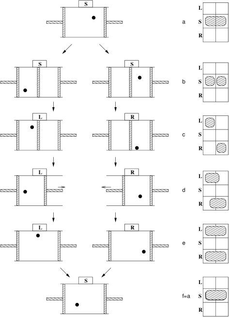
Figure 2.4: One cycle of a Szilard engine operation (after [64]). On the right is a phase diagram with the Demon’s co-ordinates on the vertical axis and the box’s on the left.

Figure 2.4 is reproduced from Bennett’s paper, and follows the phase space changes through the cycle. In (a), the Demon is in a standard state and the particle is anywhere in the box; the entropy of the system is proportional to the phase space volume occupied. In (b) the partition is inserted and in (c) the Demon makes his measurement: his state becomes correlated with the state of the particle. Note that the overall entropy has not changed. Isothermal expansion takes place in (e), and the entropy of the particle+Demon increases. After expansion the Demon remembers some information, but this is not correlated to the particle’s position. In returning the Demon to his standard state in (f) we dissipate energy into the environment, increasing its entropy.

2.4.1 Erasing Information in Quantum Systems

Szilard’s analysis has been criticised by Jauch and Baron [65] for introducing an operation which cannot be treated by equilibrium statistical mechanics: at the moment when the piston is inserted the gas violates the law of Gay-Lussac [65]. These authors even go so far as to denounce any relation between thermodynamic entropy and informational entropy, much to the peril of the author of the current chapter.

However, a more careful quantum analysis of Szilard’s engine supports Szilard’s idea of a connection between these concepts. Zurek [66] has performed this analysis. He considers a particle in an infinite square well potential of width $L$, and the piston is replaced by a slowly inserted barrier of width $\delta\ll L$ and height $U\gg kT$. The main result is that, in an appropriate limit, the system can at all times be described by its partition function $Z$: the thermodynamic approximation is valid. Zurek then analyses a “classical” demon to illustrate that Szilard’s conclusion is correct if the Second Law is valid, and a “quantum” demon which explicitly has to reset itself and so demonstrates that Bennett’s conclusion regarding the destination of the excess entropy is also correct.

The moral of the story is that erasure of information is a process which costs free energy — or equivalently, which causes an increase in overall entropy. This is useful for us, because if we can find a way to efficiently erase information (i.e. to saturate the bound in Landauer’s principle) then we can give a physical interpretation of the Holevo bound.

Plenio [67], exploiting an erasure protocol described by Vedral [68], gives such an optimal erasure protocol based on placing the demon (or the measurement apparatus) in contact with a heat bath with an appropriate density operator. Plenio then describes two ways to erase information (illustrated in Figure 2.5).

Figure 2.5: Two ways of erasing information.

Alice and Bob are going to communicate by sending mixed states from the ensemble $\{\rho_{i};p_{i}\}$ (so the overall state is $\rho=\sum p_{i}\rho_{i}$. However, Alice is feeling whimsical: she decides to send pure states $|\phi^{i}_{k}\rangle$ drawn from a probability distribution $r^{i}_{k}$. These pure states are chosen so that $\rho_{i}=\sum_{k}r^{i}_{k}|\phi^{i}_{k}\rangle\langle\phi^{i}_{k}|$. Once Bob receives the system, he can erase the information in one of two ways: (1) by directly erasing all the pure states or (2) by first erasing the irrelevant information regarding which pure state he received (a) and then erasing the resulting known mixed state.

By erasing in one step, Bob incurs an entropy cost $S_{1}=S(\rho)$ since he has erased efficiently. In part (b) of the second step, he incurs a cost $S_{2b}^{i}=S(\rho_{i})$ when erasing a particular message $\rho_{i}$, after determining that this was indeed the message Alice sent. However, on average this step will cost Bob $S_{2b}=\sum_{i}p_{i}S(\rho_{i})$. The best Bob can therefore do on step 2(a) is the difference:

$$S_{2a}=S_{1}-S_{2b}.$$ (2.66)

But Landauer’s principle tells us that the best measurement Bob makes to determine the value of $i$ that Alice sent can yield no more information that the entropy of erasure:

$$I\leq S_{2a}=S(\rho)-\sum_{i}p_{i}S(\rho_{i}).$$ (2.67)

We thus see that the Holevo bound, proved in Section 2.1.3, which was based on an abstract relation satisfied by the von Neumann entropy, has an interpretation in terms of a very deep principle in information physics, namely Landauer’s principle. This connection provides further support for the latter principle and possibly also some guidance for the question, still unresolved, of the capacity of a channel to transmit intact quantum states.

Chapter 3 Entanglement and Quantum Information

In the previous chapter we considered how classical information is manifested in quantum systems. One of the major results was the discrepancy between the amount of information used to prepare a quantum system, and that which can usefully be obtained from it. Clearly the concept of “classical” information is missing something, just as “classical” orbits became awkward in quantum mechanics.

A “classical” information carrier is usually a two-state system, or a system with two distinct phase space regions. This is regarded as a resource for conveying the abstract notion of a bit. By direct analogy, a two-level quantum system can be regarded as a resource for carrying one two-level quantum state’s worth of information. We call the abstract quantity embodied by this quantum resource a quantum bit, or qubit.

In this chapter we will consider the properties of quantum information. The Schumacher Coding Theorem [18] will give us a “system-independent” way of measuring information. We will discuss the relation between quantum information and quantum entanglement, and how the latter can be measured — and more importantly, what it can be used for. We will also look at whether quantum information is useful in a practical sense: can it be protected from errors?

3.1 Schumacher’s Noiseless Coding Theorem

A first question which arises is: How does Alice send quantum information to Bob? Classically, she would compress the information according to Shannon’s Noiseless Coding Theorem, encode this into the state of her classical physical systems, and convey these to Bob — we assume there is no noise in the channel they are using — who would perform an inverse operation to extract Alice’s message. In the quantum case, we immediately run into a problem. As soon as Alice attempts to determine (through measurement) her quantum state, she has lost exactly that quantum information she wished to convey to Bob — we discovered this in the previous chapter. If Alice happens to have the preparation information in classical form, she can send this to Bob; but this information can be arbitrarily large. Also, there are situations in which Alice doesn’t know what state she’s got (perhaps the state is the product of a quantum computation which now requires Bob’s input [69]).

An obvious solution is to simply convey the physical system to Bob. If for example the system is a two-level quantum system, she will incur no more effort in doing this than in conveying one classical bit of information, which also requires a two-state system. But once again we encounter a redundancy: suppose the system has four orthogonal states but we happen to know that all the “signal” quantum states Alice needs to send are contained in a two-dimensional subspace. Then sending the entire system is not necessary, since Alice could transpose the state onto a two-dimensional system without losing any of this “quantum information”. So the question is: Can we generalise this result in some way? How big does the system conveyed to Bob have to be? Does it depend on whether the quantum states Alice wants to send are pure or mixed?

The answer for pure states is that the system can be compressed to a Hilbert space of dimension $2^{S(\rho)}$, where once again $S(\rho)$ is the entropy of the signals. And for mixed states? One would be tempted to guess that the answer is similar to that for pure states, with the Holevo information substituted for the entropy, but this is not known. This is certainly a lower bound, but the question becomes rather more complicated for mixed states, as will be discussed later. But for now, before discussing Schumacher’s result, we will look at how quantum information is encoded, and what measure we will use for judging the accuracy of the decoded state.

Suppose the state Alices wants to send is in the Hilbert space $H_{M}$, which we call the message system; this could be a subspace of some larger system space as long as we know that the signals are in $H_{M}$. She wishes to transfer this quantum information to a transmission system represented by $H_{T}$. Copying the information is not allowed, but transposition is; that is, the operation

$$|a_{M},0_{T}\rangle\longrightarrow|0_{M},a_{T}\rangle$$ (3.1)

can be performed, where $|0_{M}\rangle$ and $|0_{T}\rangle$ are fixed standard states. This operation can be made unitary if $\dim H_{T}\geq\dim H_{M}$, simply by specifying the (ordered) basis in $H_{T}$ to which some (ordered) basis in $H_{M}$ gets mapped. This is the exact analogue of classical coding. Alice then passes the system $T$ to Bob, who performs an inverse swap operation onto his decoding system $H_{M^{\prime}}$ — and no quantum information has been discarded. The communication process is represented in Figure 3.1(a).

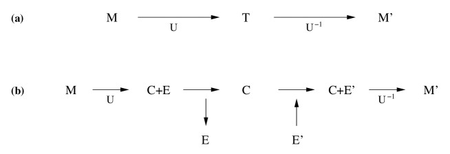
Figure 3.1: The transmission of quantum information. In (a) no information is discarded, but in (b) the communication is approximate.

If we wish to compress the information so that it occupies a smaller Hilbert space, we will have to consider an approximate transposition, as represented in Figure 3.1(b). In this case our transmission system is decomposed into a code system $H_{C}$ of dimension $d$, and an ancilla $H_{E}$. Only the code system is conveyed to Bob, and the ancilla is discarded. On the receiving end, Bob attaches an ancilla $H_{E^{\prime}}$ in a standard state and performs a decoding operation, which could be the inverse $U^{-1}$ of the coding operation. In this case the exact form of the encoding operation $U$ becomes very important; as much of the “weight” of Alice’s signal states as possible must end up in the quotient space $H_{C}$ that Bob receives, and indeed the dimension of this space must be large enough to receive almost all of the “quantum messages” Alice would like to send.

Suppose Alice sends signal states $|a_{M}\rangle$, each with probability $p(a)$. Then we can trace the path of the signal as follows:

$$|a_{M}\rangle\langle a_{M}| \longrightarrow U|a_{M}\rangle\langle a_{M}|U^{-1}=\Pi_{a}$$ (3.2)

$$\longrightarrow \mbox{Tr}_{E}\;\Pi_{a}$$

$$\longrightarrow \mbox{Tr}_{E}\;\Pi_{a}\otimes|0_{E^{\prime}}\rangle\langle 0_{E^{\prime}}|=W_{a}$$

$$\longrightarrow U^{-1}W_{a}U=\rho_{a}.$$

So the final state that Bob receives will be a mixed state.

Clearly Bob will not get all the quantum information Alice started with. But how do we measure what got to Bob? Any measure of distinguishability will work (where now Alice and Bob’s aim is clearly to minimise distinguishability). For mathematical reasons, the fidelity is usually used, and in this case it has a very convenient interpretation. Suppose that Bob knew precisely which pure state $|a_{M}\rangle$ Alice started with — for example, they are calibrating their equipment. Then there is a maximal test [6] for which the outcome can be predicted with certainty. Suppose the (mixed) state received by Bob after decoding is $\rho$; if Bob performs this maximal test on the decoded state then the probability that he will think that the state is exactly the one sent is $\mbox{Tr}\;\rho\,|a_{M}\rangle\langle a_{M}|$. This is therefore a practical measure of the accuracy of the received state. The average fidelity of the transmission is then defined as

$$\bar{F}=\sum_{a}p(a)\mbox{Tr}\;|a_{M}\rangle\langle a_{M}|\rho_{a}.$$ (3.3)

The fidelity is between 0 and 1, and equal to one if and only if all signals are transmitted perfectly, as in Figure 3.1(a). Note that the fidelity can also be computed in terms of the code system states (rather than the message and decoding systems):

$$\bar{F} = \sum_{a}p(a)\mbox{Tr}\;|a_{M}\rangle\langle a_{M}|\rho_{a}$$ (3.4)

$$= \sum_{a}p(a)\mbox{Tr}\;U^{-1}\Pi_{a}U\;U^{-1}W_{a}U$$

$$= \sum_{a}p(a)\mbox{Tr}\;\Pi_{a}W_{a}.$$

Schumacher then goes on to prove two lemmas:

Lemma 3.1.1.

Suppose that $\dim H_{C}=d+1$ and denote the ensemble of states on $M$ by $\rho_{M}=\sum p(a)|a_{M}\rangle\langle a_{M}|$. Suppose there exists a projection $\Lambda$ onto a $d$-dimensional subspace of $H_{M}$ with $\mbox{Tr}\;\rho_{M}\Lambda>1-\eta$. Then there exists a transposition scheme with fidelity $\bar{F}>1-2\eta$.

Lemma 3.1.2.

Suppose $\dim H_{C}=d$ and suppose that for any projection $\Lambda$ onto a $d$-dimensional subspace of $H_{M}$, $\mbox{Tr}\;\rho_{M}\Lambda<\eta$ for some fixed $\eta$. Then the fidelity $\bar{F}<\eta$.

Both of these results are highly plausible. The first says that if almost all of the weight of the ensemble of message states is contained in some subspace no larger than the code system, then accurate transposition will be possible. This is proved constructively by demonstrating a transposition scheme with this fidelity. The second lemma deals with the situation in which any subspace of the same size as code system doesn’t contain enough of the message ensemble, in which case the fidelity is bounded from above.

No mention is made in these lemmas of the ensemble of states comprising $\rho_{M}$; they could be arbitrary states, or they could be the eigenstates of $\rho_{M}$; but according to the lemma the transposition fidelity can always be bounded as appropriate. Focus is thus shifted away from the ensemble, and all we have to deal with is the density operator $\rho_{M}$. Schumacher’s theorem then says:

Theorem 3.

Quantum Noiseless Coding Theorem [18] Let $M$ be a quantum signal source with a signal ensemble described by the density operator $\rho_{M}$ and let $\delta,\epsilon>0$.

(i) Suppose that $S(\rho_{M})+\delta$ qubits are available per signal. Then for sufficiently large $n$, groups of $n$ signals can be transposed via the available qubits with fidelity $\bar{F}>1-\epsilon$.

(ii) Suppose that $S(\rho_{M})-\delta$ qubits are available for coding each signal. Then for sufficiently large $n$, if groups of $n$ signals are transposed via the available qubits, then the fidelity $\bar{F}<\epsilon$.

To prove this, we begin by noting that the maximum value of $\mbox{Tr}\;\rho_{M}\Lambda$ is realised when $\Lambda$ is a projection onto the subspace spanned by eigenstates of $\rho_{M}$ with the largest eigenvalues. Now, as in the case of the classical theorem, we consider block coding i.e. we focus on the density operator $\rho^{N}=\rho\otimes\ldots\otimes\rho$. The eigenvalues of this operator are products of the single system eigenvalues. As in the discussion of the law of large numbers following Eqn 1.18, we can find a set of approximately $2^{n[s(\rho_{M})+\delta]}$ such product eigenvalues with total sum $>1-\epsilon/2$. Then by Lemma 1, there is a transposition scheme with fidelity $\bar{F}>1-\epsilon$.

Conversely, if we can only add together $2^{n[S(\rho_{M})-\delta]}$ of the largest eigenvalues, this sum can be made arbitrarily small (see for example [18], [8]). Hence any projection onto a subspace of this size will yield arbitrarily low fidelity.

Schumacher’s result is valid for unitary encoding and decoding operations. In full generality, one should allow Alice and Bob to perform any operation (represented by a superoperator) on their systems and check whether further compression can be achieved than discussed above. This was considered by Barnum et al [37], who showed that Schumacher coding gives the maximum possible compression. In particular, they showed that even if Alice has knowledge of which state she is sending, and applies different encodings depending on this knowledge, she can do no better than if she coded without knowledge of the signals.

3.1.1 Compression of Mixed States

What is the optimal compression for ensembles of mixed states? That is, what size Hilbert space do we need to communicate signals from the ensemble $\{\rho_{a};p_{a}\}$ accurately? Once again, we will measure accuracy using the fidelity, although in this case we must use the form for mixed states given in Eqn 2.64.

The protocol for pure state compression suggested by Jozsa and Schumacher in [71] can also be applied to mixed state ensembles, and compresses an ensemble down to the value of its von Neumann entropy. However, it is very simple to show that this is not optimal, simply by considering an ensemble of mixed states with disjoint support. In this case our coding technique could be simply to measure the system — we can distinguish perfectly between signal states since they are disjoint — and prepare it in a pure state, such that the ensemble of pure states has lower entropy

For the problem of mixed state compression, the signal ensemble is ${\cal E}^{0}=\{\rho_{a};p_{a}\}$, where the $\rho_{a}$ are now mixed states. In order to code this, Alice accumulates a block of $n$ signals $\rho_{a_{1}}\otimes\ldots\otimes\rho_{a_{n}}=\sigma_{\bf a}$, where ${\bf a}$ is a multiple index. The block ensemble is ${\cal E}_{n}=\{\sigma_{\bf a};q_{\bf a}\}$, where $q_{\bf a}$ is a product of the appropriate $p$ probabilities, and it has a density matrix $\rho_{n}=\sum_{\bf a}q_{\bf a}\rho_{\bf a}$. Alice will perform some operation on these states to code them.

We now have to distinguish two types of coding: if Alice knows which states she is sending to Bob, then she can code each state differently and we call this arbitrary or nonblind coding; if she doesn’t know then she treats all states equally, which is called blind coding. Alice’s allowed operations, in the case of blind coding, are completely positive maps (represented by superoperators). For arbitrary coding, she can use any map; she could even, if she wanted, replace each code state $\rho_{\bf a}$ by a pure state $|\psi_{\bf a}\rangle$. Bob, on the other hand, is always constrained to using a completely positive map, since he can have no knowledge of the state he receives.

A protocol is then defined as a sequence $(\Lambda_{n},\$_{n})$ of Alice’s encoding operations $\Lambda_{n}$ and Bob’s decoding superoperators $\$_{n}$ which yield arbitrarily good fidelity as block size increases i.e.

$$\bar{F}_{n}=\sum_{\bf a}F\big{(}\rho_{\bf a},\$_{n}\left[\Lambda_{n}(\rho_{\bf a})\right]\big{)}$$ (3.5)

satisfies $\bar{F}_{n}\rightarrow 1$ as $n\rightarrow\infty$. The rate of a protocol ${\cal P}$ is

$$R_{\cal P}=\lim_{n\rightarrow\infty}\frac{1}{n}\log\dim\tilde{\rho},$$ (3.6)

where $\dim\tilde{\rho}$ is the dimension of the support of $\tilde{\rho}$.

Horodecki then distinguishes between the passive information $I_{p}=\inf_{\cal P}R_{\cal P}$ where the infimum is taken over all blind protocols (where $\Lambda_{n}$ is a superoperator), and the effective information $I_{e}$ which is defined similarly but with the infimum taken over arbitrary protocols (where $\Lambda_{n}$ is an arbitrary map). Clearly $I_{e}\leq I_{p}$ since all blind protocols are also arbitrary. Horodecki [42] shows that the effective information is bounded below by the Holevo information, $\chi({\cal E})\leq I_{e}$, and notes that the bound can be achieved if the ensemble $\tilde{\cal E}$ of code system states has asymptotically vanishing mean entropy (the code states become almost pure). We may also consider the “information defect” $I_{d}=I_{p}-I_{e}$, which characterises the stinginess of the ensemble: a nonzero $I_{d}$ indicates that more resources are needed to convey the quantum information than the actual value of the information. It is not known if the information defect is ever nonzero.

A tantalising clue is given in Schumacher’s original paper where he showed that entanglement could be compressed using his protocol. Suppose Alice and Charlie share an EPR pair between them; for definiteness, suppose each of them holds an electron and the joint state of the electrons is

$$|\psi^{-}\rangle=\frac{1}{\sqrt{2}}\left(|\!\uparrow\rangle_{A}|\!\downarrow\rangle_{C}-|\!\downarrow\rangle_{A}|\!\uparrow\rangle_{C}\right)$$ (3.7)

($|\!\uparrow\rangle$ and $|\!\downarrow\rangle$ refer to spin polarisation states of the electrons). It is well-known that such a state exhibits strong correlations (see e.g. Bell [72]). The question is, do such correlations persist between Bob and Charlie if Alice conveys her system to Bob using the methods above? Schumacher showed that they do. We are in effect conveying the full pure state $|\psi^{-}\rangle$ to Bob, but only compressing one half of it — Charlie’s half undergoes the identity transformation. This can be done with arbitrarily good fidelity, so the correlations between Bob and Charlie will be arbitrarily close to the original EPR correlations.

Horodecki [73] then showed that in full generality, the problem of arbitrary (nonblind) compression of an ensemble of mixed states could be reduced to minimising the entropy of any extension ensemble. An extension of density operator $\rho$ is a density operator $\sigma$ over a larger Hilbert space with the property that $\rho=\mbox{Tr}_{\mbox{\scriptsize ancilla}}\;\sigma$, and the extension of an ensemble is another ensemble with the same probabilities whose elements are extensions of the original. In particular, it seems fruitful to investigate the purifications of a given ensemble — since any purification is also an extension. We would then be able to use the provably optimal techniques of pure state coding to solve the problem. This is extremely handy reduction, enabling us to ignore the unwieldy representation of protocols and focus on states and their purifications.

However, minimisation of von Neumann entropy $S$ over all extensions is also a very difficult problem. A first, and counter-intuitive, result was that of Jozsa and Sclienz [34] mentioned in Sec. 2.2. Suppose we start with a particular purification of ${\cal E}$ and ask how we can distort the states, leaving the probabilities fixed, to decrease $S$. A reasonable first guess, based on our knowledge of two-state ensembles, is that any distortion which increases pairwise overlap will decrease von Neumann entropy. As disussed previously, Jozsa and Schlienz showed that the von Neumann entropy of almost any pure state ensemble in more than two dimensions can be increased by making all the states more parallel. The compressibility — and the distinguishability — are global properties of the ensemble which cannot be reduced to accumulated local properties of members of the ensemble.

There are still many unanswered questions in this area, and many tantalising clues. Several of these clues, together with some partial results have been collected together by Barnum, Caves, Fuchs, Jozsa and Schumacher [74]. One of their most striking insights is that the fidelity between two strings of states $\rho_{\bf a}$ and $\sigma_{\bf a}$ depends on whether we are content to compute the fidelity of each state as it arrives (LOCAL-FID) or whether we compute the fidelity of blocks of states (GLOBAL-FID). The latter is a stringer condition that (LOCAL-FID) since it not only requires the individual states to be very similar but also their entanglements should not be altered. For pure states the two types of fidelity are the same, but for mixed states Barnum et al exhibit an example with high (LOCAL-FID) but zero (GLOBAL-FID).

An important bound proved by Barnum et al [74] is that the Holevo information is a lower bound for compression under the criterion (GLOBAL-FID), although there are strong reasons to believe that under this fidelity criterion this bound is not generally attainable, but it has been shown that for a weaker fidelity this bound can always be achieved [75]. At the moment there appear to be too many trees for us to see the wood in mixed state compression.

3.2 Entanglement

Entanglement is one of the most intruiging aspects of quantum theory. First labeled verschränkung by Schrödinger [76], entanglement became one of the features most uncomfortable to Einstein. It was the paper by Einstein, Podolsky and Rosen [77] (describing the famous EPR paradox) which expressed some of this dissatisfaction with the “action at a distance” of quantum mechanics. The crucial blow to Einstein’s requirement of “local reality” came from John Bell in 1964 [72], and a version of Bell’s theorem will be mentioned below.

First, however, we look at what entanglement is; and we begin by looking at the canonical example of entangled qubits. Suppose we are considering two electrons $A$ and $B$; then a basis for the electron spin states is

$$|\phi^{+}\rangle=\frac{1}{\sqrt{2}}\left(|\!\uparrow\uparrow\rangle+|\!\downarrow\downarrow\rangle\right)$$

$$|\psi^{+}\rangle=\frac{1}{\sqrt{2}}\left(|\!\uparrow\downarrow\rangle+|\!\downarrow\uparrow\rangle\right)$$

$$|\phi^{-}\rangle=\frac{1}{\sqrt{2}}\left(|\!\uparrow\uparrow\rangle-|\!\downarrow\downarrow\rangle\right)$$

$$|\psi^{-}\rangle=\frac{1}{\sqrt{2}}\left(|\!\uparrow\downarrow\rangle-|\!\downarrow\uparrow\rangle\right)$$

where, for example, we denote the state $|\!\uparrow\rangle_{A}\otimes|\!\downarrow\rangle_{B}$ by $|\!\uparrow\downarrow\rangle$. These states form the Bell basis (or alternatively they are EPR pairs), and they have numerous interesting properties that will be briefly discussed here.

A bipartite system in a Bell state has a peculiar lack of identity. If we consider just one half of the system and trace out the other system’s variables, we find

$$\mbox{Tr}_{A}\;|\Upsilon\rangle\langle\Upsilon| = {}_{A}\langle\uparrow\!|\Upsilon\rangle\langle\Upsilon|\!\uparrow\rangle_{A}+{}_{A}\langle\downarrow\!|\Upsilon\rangle\langle\Upsilon|\!\downarrow\rangle_{A}$$ (3.8)

$$= \frac{1}{2}\leavevmode\hbox{\small 1\kern-3.8pt\normalsize 1}=\mbox{Tr}_{B}\;|\Upsilon\rangle\langle\Upsilon|$$ (3.9)

(where $|\Upsilon\rangle$ is one of the Bell states): so any orthogonal measurement on a single particle will yield a completely random outcome. Of course neither half of the system, considered alone, is in a pure state — so despite the fact that we have maximal information about both systems, there is no test we can perform on either one which will yield a definite outcome. Each of the basis states represents (optimally) two bits of information, which we may conveniently call the amplitude bit (the $|\psi\rangle$ states both have amplitude 0, the $|\phi\rangle$ states 1) and the phase bit (the $+$ states have phase 0, the $-$ states have phase 1). The amplitude bit is the eigenvalue of the observable $\sigma_{x}^{A}\sigma_{x}^{B}$ and the phase bit of the observable $\sigma_{z}^{A}\sigma_{z}^{B}$ — and these are commuting operators. The problem in determining their identity comes when the systems $A$ and $B$ are spatially separated, because the local operators $\sigma_{x}^{A}$ and $\sigma_{x}^{B}$ which could be used to discover the amplitude bit do not commute with the phase operator $\sigma_{z}^{A}\sigma_{z}^{B}$. Determining the amplitude bit through local measurements will disturb the phase bit; so the information is practically inaccessible. If the particles are brought together, we can measure the amplitude bit without determining the values of $\sigma_{x}$ individually, and hence fully determine the identity of the state.

So: what makes these states entangled? And what other states are entangled? The answer to these questions is rather an answer in the negative: a pure state is not entangled (i.e. it is separated) if it can be written as a product state over its constituent subsystems (we will mention mixed state entanglement later). An alert student may protest that by changing bases we could change a state from entangled to separated – so we should be sure of our facts first.

Suppose $|\Psi\rangle$ is a pure state over two subsystems $A$ and $B$ (that is, it is a vector from $H_{A}\otimes H_{B}$). Then let $\{|i\rangle\}$ be the basis for $H_{A}$ in which the reduced density matrix for subsystem $A$ is diagonal:

$$\rho_{A}=\mbox{Tr}_{B}\;|\Psi\rangle\langle\Psi|=\sum_{i}\lambda_{i}|i\rangle\langle i|.$$ (3.10)

Of course if $\{|\alpha\rangle\}$ is any basis for $H_{B}$, then we can write

$$|\Psi\rangle=\sum_{i,\alpha}a_{i,\alpha}|i\rangle\otimes|\alpha\rangle=\sum_{i}|i\rangle\otimes|\tilde{i}\rangle$$ (3.11)

where we have defined $|\tilde{i}\rangle=\sum_{\alpha}a_{i,\alpha}|\alpha\rangle$. The $|\tilde{i}\rangle$ do not necessarily form an orthonormal basis, but we can calculate $A$’s reduced density matrix in terms of them:

$$|\Psi\rangle\langle\Psi| = \sum_{i,j}|i\rangle_{A}|\tilde{i}\rangle_{B}\;{}_{A}\langle j|{}_{B}\langle\tilde{j}|$$ (3.12)

$$\Rightarrow\rho_{A} = \sum_{k}{}_{B}\langle k|\Psi\rangle\langle\Psi|k\rangle_{B}$$ (3.13)

$$= \sum_{i,j}{}_{B}\langle k|\tilde{i}\rangle_{B}\;{}_{B}\langle\tilde{j}|k\rangle_{B}\;|i\rangle_{A}{}_{A}\langle j|$$ (3.14)

$$= \sum_{i,j}\langle\tilde{j}|\tilde{i}\rangle\;|i\rangle\langle j|$$ (3.15)

where $\{|k\rangle_{B}\}$ is any orthonormal basis for $H_{B}$. Comparing this with Eqn 3.10, we see that

$$\langle\tilde{j}|\tilde{i}\rangle=\lambda_{i}\delta_{ij}:$$ (3.16)

the $|\tilde{i}\rangle$ are orthogonal! Defining $\sqrt{\lambda_{i}}|i^{\prime}\rangle=|\tilde{i}\rangle$ (an orthonormal basis) we find that

$$|\Psi\rangle=\sum_{i}\sqrt{\lambda_{i}}|i\rangle\otimes|i^{\prime}\rangle.$$ (3.17)

This is called the Schmidt decomposition of the bipartite state $|\Psi\rangle$. Notice that this decomposition is unique, and tells us also that the reduced density matrices $\rho_{A}$ and $\rho_{B}$ have the same non-zero eigenvalue spectrum — if $H_{A}$ and $H_{B}$ have different dimensions, then the remaining eigenvalues are zero. The Schmidt decomposition is related to a standard result in linear algebra, known as the singular value decomposition.

We now have a very simple method of defining whether a pure state is entangled. Define the Schmidt number $N_{S}$ to be the number of non-zero terms in the expansion Eqn 3.17. Then the state is entangled if $N_{S}>1$. The special features of such entangled states are related to Bell’s theorem.

Bell’s Theorem

Einstein and others thought that, although quantum physics appeared to be a highly accurate theory, there was something missing. One proposed way of remedying this problem was to introduce hidden variables; variables lying at a deeper level than the Hilbert space structure of quantum mechanics, and to which quantum theory would be a statistical approximation. The idea is then that quantum mechanics describes a sort of averaging over these unknown variables, in much the same way as thermodynamics is obtained from statistical mechanics. In fact, the variables could even in principle be inaccessible to experiment: the important feature is that these variables would form a complete description of reality. Of course, to be palatable we should require these variables to be constrained by locality, to make the resulting theory “local realist”. In the words of Einstein [78, p. 85]:

But on one supposition we should, in my opinion, absolutely hold fast: the real factual situation of the system $S_{2}$ is independent of what is done with the system $S_{1}$, which is spatially separated from the former.

Einstein was convinced that the world was local, deterministic and real.

John Bell [72] struck a fatal blow to this view. Bell considered a very simple inequality which any local deterministic theory must obey — an inequality that was a miracle of brevity and could be explained to a high school student, and was indeed known to the $19^{\rm th}$ century logician Boole [79] — and he showed that quantum mechanics violates this inequality. We are thus forced to one of several possible conclusions: (i) quantum mechanics gives an incorrect prediction, and a “Bell-type” experiment will demonstrate this; (ii) quantum mechanics is correct, and any deterministic hidden variable theory replicating the predictions of quantum mechanics must be non-local. With the overwhelming experimental evidence supporting quantum mechanics, it would be a foolhardy punter who put his money on option (i), and indeed several Bell-type experiments performed to date have agreed with the quantum predictions [80]. Bell’s theorem refers to the conclusion that any deterministic hidden variable theory that reproduces quantum mechanical predictions must be nonlocal.

An excellent discussion of Bell’s theorem and its implications is found in [6, Ch. 6]. Several papers have since appeared on “Bell’s theorem without inequalities” (for a readable discussion, see [81]), which eliminate the statistical element of the argument and make Bell’s theorem purely logical. In this case a single outcome of a particular quantum mechanical experiment is enough to render a hidden variable description impossible.

The importance of entangled states, as defined above, is that every entangled pure state violates a Bell inequality [82]. However, the definition of entangled states given above is not very helpful when we need to compare the degree of entanglement of bipartite states. However, we have all we need to find a quantitative measure of entanglement: a probability distribution, given by the eigenvalues $\lambda_{i}$. We define the entanglement of a bipartite state $|\Psi\rangle$ to be

$$E(|\Psi\rangle) = H(\lambda_{i})$$ (3.18)

$$= S(\rho_{A})=S(\rho_{B})$$ (3.19)

where $H$ is the familiar Shannon entropy. Happily, the entanglement of a state with $N_{S}=1$ is zero. The maximally entangled states are those of the form $\sum_{i}|i\rangle|i^{\prime}\rangle/\sqrt{N}$ which are equal superpositions of orthogonal product states. The Bell state basis consists of maximally entangled states, and these are the only maximally entangled states of two qubits. In analogy with the primitive notion of a qubit being a measure of quantum entanglement, we define an ebit to be the amount of entanglement shared between systems in a Bell state.

Bennett et al [47] point out that this entanglement measure has the pleasing properties that (1) the entanglement of independent systems is additive and (2) the amount of entanglement is left unchanged under local unitary transformations, that is, those that can be expressed as products: $U=U_{A}\otimes U_{B}$. The entanglement cannot be increased by more general operations either (see below), and has a convenient interpretation that one system with entanglement $E=E(|\Psi\rangle)$ is completely equivalent (in a sense to be made clear later) to $E$ maximally entangled qubits.

Mixed state entanglement

The case for “a measure of entanglement” of a bipartite mixed state $\rho_{AB}$ is not quite as clear cut. Indeed, just about the only useful definition is that of a separable state, which is one which can be written as

$$\rho_{AB}=\sum_{i}p_{i}\;\rho_{A}^{i}\otimes\rho_{B}^{i}.$$ (3.20)

We will return to measures of entanglement for mixed states later, once we have developed more practical notions of the uses of entanglement and an idea of what we are in fact hoping to quantify. For now, we turn our attention to these issues.

3.2.1 Quantum Key Distribution (again)

We have already seen a protocol for QKD in Section 2.3. Here we describe a variant based on Bell states, due to Ekert [83] which illustrates the interchangeability of quantum information with entanglement.

The protocol is illustrated in Figure 3.2.

Figure 3.2: Illustration of quantum key distribution using EPR pairs.

We assume Alice and Bob start off sharing a large number $n$ of Bell state pairs, which we will assume are the singlet state $|\psi^{-}\rangle$. These pairs could be generated by a central “quantum software” distributor and delivered to Alice and Bob, or Alice could manufacture them and transmit one half of each pair to Bob. Once again, Alice and Bob have written down strings of $n$ digits, but this time the digits could be 0, 1 or 2 — and once again, 0, 1 and 2 correspond to different nonorthogonal measurement bases (these bases are illustrated for spin-1/2 measurements in Figure 3.2). The outcome of any measurement is either “$+$” or “$-$”.

We denote by $P_{-+}(i,j)$ the probability that Alice gets a “$-$” when measuring in the $i$ basis at the same time as Bob finds “$+$” in the $j$ basis. The correlation coefficient between two measurement bases is

$$E(i,j)=P_{++}(i,j)+P_{--}(i,j)-P_{+-}(i,j)-P_{-+}(i,j).$$ (3.21)

If we do the calculations we find for our choice of bases

$$E(i,j)=-{\bf a}_{i}\cdot{\bf b}_{j},$$ (3.22)

where ${\bf a}_{i}$ and ${\bf b}_{j}$ are the direction vectors of the “$+$” outcomes of Alice’s $i^{\rm th}$ and Bob’s $j^{\rm th}$ basis respectively. (For example, ${\bf a}_{0}=(0,1)$ and ${\bf b}_{0}=(\frac{1}{\sqrt{2}},\frac{1}{\sqrt{2}})$.) So we define the quantity

$$S=E(0,0)-E(0,2)+E(2,0)+E(2,2)$$ (3.23)

and calculate that for the bases illustrated in Figure 3.2, $S=-2\sqrt{2}$. The quantity $S$ is a generalisation, due to Clauser, Horne, Shimony and Holt [84], of the correlation function originally used by Bell.

Once Alice and Bob have made all their measurements on the EPR pairs, they announce their measurement bases (i.e. their random strings of 0, 1 and 2). The only cases in which their measurements will agree are (i) Alice measured in basis 1 and Bob in basis 0; (ii) Alice measured in basis 2 and Bob basis 1. They will thus know that when these measurements were made they got anti-correlated results, and they can use this to generate a secret key. And how can they tell if someone was eavesdropping? This is where the quantity $S$ comes in. Notice that $S$ is defined only for cases where the measurement bases were different. Bob can publicly announce all his measurement results for when both their bases were either 0 or 2, and Alice can use this to calculate the correlation functions and hence $S$. Since $S$ is bounded by $-2\sqrt{2}\leq S\leq 2\sqrt{2}$, any intereference by an eavesdropper will reduce the (anti)correlation between Alice and Bob’s measurements and hence be statistically detectable (although this is quite difficult to prove; see [85]). In this case Alice will abort the key distribution.

A useful aspect of this protocol is that the “element of reality” from which the secret key is constructed does not come into existence until Alice and Bob make their measurements. This contrasts with the BB84 scheme of Section 2.3, in which Alice is required to impose a known state onto the quantum system she sends to Bob. Practically, this means that the BB84 protocol is vulnerable to someone breaking into Alice’s safe and (without being detected by Alice) stealing the preparation basis information — in which case the eavesdropper simply needs to wait for Alice and Bob’s measurement basis announcement and can calculate the secret key. In Ekert’s protocol Alice and Bob can hold onto their EPR pair until they need a key, then use the protocol, send the message and destroy the key all within a short time.

3.2.2 Quantum Superdense Coding

Quantum information can also be used to send classical information more efficiently. This is known as quantum superdense coding, and is due to Bennett and Wiesner [86].

Suppose Alice wanted to send two bits of classical information to Bob. One way she could do this is by sending him two electrons with information encoded in their polarisation states — and as we’ve seen already, two bits is the maximum amount of classical information she can send in this way. One method of doing this would be, for example, to send one of the states $|\psi^{+}\rangle$, $|\psi^{-}\rangle$, $|\phi^{+}\rangle$ or $|\phi^{-}\rangle$ each with probability $1/4$.

Suppose instead that Alice and Bob share the Bell state $|\phi^{+}\rangle$. Define the following local actions which Alice can perform on her side of the pair: $U_{0}=\leavevmode\hbox{\small 1\kern-3.8pt\normalsize 1}\otimes\leavevmode\hbox{\small 1\kern-3.8pt\normalsize 1}$, $U_{1}=\sigma_{x}\otimes\leavevmode\hbox{\small 1\kern-3.8pt\normalsize 1}$, $U_{2}=\sigma_{y}\otimes\leavevmode\hbox{\small 1\kern-3.8pt\normalsize 1}$ and $U_{3}=\sigma_{z}\otimes\leavevmode\hbox{\small 1\kern-3.8pt\normalsize 1}$. The effects of the operations on the shared EPR pair can be calculated:

$$U_{0}|\phi^{+}\rangle=|\phi^{+}\rangle U_{1}|\phi^{+}\rangle=|\psi^{+}\rangle$$

$$U_{2}|\phi^{+}\rangle=-i|\psi^{-}\rangle U_{3}|\phi^{+}\rangle=|\phi^{-}\rangle.$$

A method for sending information suggests itself: Alice and Bob take out their old EPR pairs, which they’ve had for years now, and Alice performs one of these operations on her side of the pair. She then sends her one electron to Bob, who makes the measurements $\sigma_{x}^{A}\sigma_{x}^{B}$ and $\sigma_{z}^{A}\sigma_{z}^{B}$ on the two electrons now in his possession. As mentioned previously (Section 3.2), all the Bell states are simultaneous eigenstates of these operators corresponding to different eigenvalues, so these measurements completely identify the state. From this outcome he can infer which of the four local operations Alice used. He has received two bits of information despite the fact that Alice only sent him one two-level system!

One might argue that this still requires the transmission of both halves of the EPR pair and so we don’t really gain anything — we send two two-level systems and get two bits of information. The important point here is that the shared EPR pair is a prior resource which exists before the classical information needed to be communicated. Once Alice knew the outcome of the soccer match she wanted to report to Bob, she only needed to send him one qubit.

What is the maximum “compression factor” possible? And what other states can be used for superdense coding? Hausladen et al [31] showed that any pure entangled state can be used for superdense coding, and that the maximum information that can be superencoded into a bipartite state $|\Psi_{AB}\rangle$ is $E(|\Psi_{AB}\rangle)+\log N$, where $N$ is the dimension of the system Alice sends to Bob. Clearly by sending one $N$-state system Alice can communicate $\log N$ bits of information; the excess from superdense coding is exactly equal to the entanglement of the state.

3.2.3 Quantum Teleportation

What is so special about collective measurements, and can we draw a line between what is possible with separate and with joint measurements? As mentioned earlier, no local (separated) measurements on a system in one of the Bell states can identify which Bell state it is. Similarly, Peres and Wootters [28] showed an explicit situation in which the accessible information from a set of states appeared to be higher using a joint measurement than using any set of separated measurements. In an attempt “to identify what other resource, besides actually being in the same place, would enable Alice and Bob to make an optimal measurement” [87, p. 1071] on a bipartite system, Bennett et al stumbled across the idea of quantum teleportation.

We suppose, as before, that Alice and Bob share an EPR pair which we suppose to be the state $|\phi^{+}\rangle_{AB}$. Alice is also holding a quantum state $|\mu\rangle=a|\!\uparrow\rangle_{C}+b|\!\downarrow\rangle_{C}$ of another qubit which we call system $C$. Alice might not know $a$ and $b$, and measuring the state will destroy the quantum information. However, she notices something beautiful about the state of the three particles $A$, $B$ and $C$ considered together:

$$|\phi^{+}\rangle_{AB}|\mu\rangle_{C} = \frac{1}{\sqrt{2}}\big{(}a|\!\uparrow_{A}\uparrow_{B}\uparrow_{C}\rangle+a|\!\downarrow_{A}\downarrow_{B}\uparrow_{C}\rangle+b|\!\uparrow_{A}\uparrow_{B}\downarrow_{C}\rangle+b|\!\downarrow_{A}\downarrow_{B}\downarrow_{C}\rangle\big{)}$$ (3.28)

$$= \begin{array}[t]{cccc}\frac{1}{2\sqrt{2}}\bigg{\{}&&|\phi^{+}\rangle_{AC}\;\big{(}a|\!\uparrow\rangle_{B}+b|\!\downarrow\rangle_{B}\big{)}&\\[-5.69054pt] &+&|\phi^{-}\rangle_{AC}\;\big{(}a|\!\uparrow\rangle_{B}-b|\!\downarrow\rangle_{B}\big{)}&\\ &+&|\psi^{+}\rangle_{AC}\;\big{(}b|\!\uparrow\rangle_{B}+a|\!\downarrow\rangle_{B}\big{)}&\\[-5.69054pt] &+&|\psi^{-}\rangle_{AC}\;\big{(}b|\!\uparrow\rangle_{B}-a|\!\downarrow\rangle_{B}\big{)}&\bigg{\}}.\end{array}$$

Thus if Alice performs a Bell basis measurement on the system $AC$, she projects the system into a state represented by one of the terms in Eqn 3.28. In particular, Bob’s half of the EPR pair will be projected into something that looks similar to the original state of $|\mu\rangle_{C}$ — in fact, by applying one of the operators $\leavevmode\hbox{\small 1\kern-3.8pt\normalsize 1},\sigma_{x},\sigma_{y},\sigma_{z}$ Bob can rotate his qubit to be exactly $|\mu\rangle$!

The protocol runs as follows: Alice measures the system $AC$ in the Bell basis, and gets one of four possible outcomes, and communicates this outcome to Bob. Once Bob knows the result of Alice’s measurement — and not before this — he performs the appropriate operation on his qubit and ends up with the state $|\mu\rangle$.

There are many remarkable features to this method of communication. Firstly, as long as Alice and Bob can reliably store separated EPR particles and can exchange classical information, they can perform teleportation. In particular, there can be all manner of “noise” between them (classical information can be made robust to this noise) and an arbitrarily large distance. Alice doesn’t even need to know where Bob is, as she would if she wished to send him a qubit directly — she merely needs access to a broadcasting channel.

Secondly, the speed of transmission of the state of a massive particle is limited only by the speed of classical communication — which in turn is limited only by the speed of light. This is an intriguing subversion of the idea that massive particles must travel slower than light speed, although of course, only the state is transmitted. We could even imagine a qubit realised as an electron in system $C$ and as a photon in system $B$, in which case we teleport a massive particle onto a massless particle. Quantum information is a highly interchangeable resource!

Thirdly, we have developed a hierarchy of information resources. The lowest resource is a classical bit which cannot generally be used to share quantum information and which cannot be used to create entanglement (which is a consequence of Bell’s theorem). The highest resource is a qubit, and an ebit is intermediate. This classification follows from the fact that if Alice and Bob can reliably communicate qubits, they can create an ebit entanglement (Alice simply creates an EPR pair and transmits half to Bob); whereas if they share an ebit they further require classical information to be able to transmit qubits.

Much work has been performed in attempting to implement quantum teleportation in the laboratory, with varying claims to success. Some of the techniques used are cavity QED [88], parametric down-conversion of laser light [89] and NMR [90]. Experiments are however fraught with complications, both practical and theoretical; see [91] and references therein.

Entanglement swapping

Quantum teleportation can also be used to swap entanglement [92]. Suppose Alice and Bob share the EPR pair $|\phi^{+}\rangle$ and Charlie and Doris share another $|\phi^{+}\rangle$. Then the state they have can be rewritten as

$$|\phi^{+}\rangle_{AB}|\phi^{+}\rangle_{CD} = \frac{1}{2}\big{(}|\!\uparrow_{A}\uparrow_{B}\uparrow_{C}\uparrow_{D}\rangle+|\!\uparrow_{A}\uparrow_{B}\downarrow_{C}\downarrow_{D}\rangle+|\!\downarrow_{A}\downarrow_{B}\uparrow_{C}\uparrow_{D}\rangle+|\!\downarrow_{A}\downarrow_{B}\downarrow_{C}\downarrow_{D}\rangle\big{)}$$ (3.29)

$$= \frac{1}{2}\big{(}|\phi^{+}\rangle_{AD}|\phi^{+}\rangle_{BC}+|\phi^{-}\rangle_{AD}|\phi^{-}\rangle_{BC}$$

$$\;+|\psi^{+}\rangle_{AD}|\psi^{+}\rangle_{BC}+|\psi^{-}\rangle_{AD}|\psi^{-}\rangle_{BC}\big{)}.$$

So if Bob and Charlie get together and make a Bell basis measurement on their qubits, they will get one of the four outcomes with equal probability. Once they communicate this classical information to Alice and Doris, the latter will know that they are holding an EPR pair — and Alice can convert it to $|\phi^{+}\rangle$ by a local rotation.

Of course, all that Bob has done is to teleport his entangled state onto Doris’ system, so entanglement swapping is not much different to straightforward teleportation. But entanglement swapping will be important later when we discuss quantum channels.

3.3 Quantum Computing

The theory of computing dates from work by Turing and others in the 1930’s. However the idea of a computer, as enunciated by Turing, suffered from the same shortcoming as classical information: there was no physical basis for the model. And there were surprises in store for those who eventually did investigate the physical nature of computation.

Turing wanted to formalise the notion of a “computation” as it might be carried out by a mathematician in such a way that a machine could carry out all the necessary actions. His model was a mathematician sitting in a room with access to an infinite amount of paper, some of which contains the (finite) description of the problem he is to solve. The mathematician is supposed to be in one of a finite number of definite states, and he changes state only after he reads part of the problem statement — and as he changes state he is allowed to write on the paper. A Turing machine (illustrated in Figure 3.3)

Figure 3.3: A Turing machine.

is the machine version of this mathematician. The Turing machine (TM) has a finite number of internal states, here labeled $a,b,\ldots,l$; a “read” head; and a “write” head. An infinite strip of paper, with discrete cells on it, runs between the read and write heads; each cell can either contain a 0, a 1 or a blank. Initially the paper is completely blank except for a finite number of cells which contain the problem specification. A cycle of the machine consists of reading the contents of the current cell, writing a new value into the cell, changing state, and moving the tape left or right. For example, consider the instruction set shown in the figure. The machine is currently in the state $a$ and is reading the value 0; according to the instructions given, the machine should write a 1, change into state $g$ and shift the tape to the left so that the read head sees a 1.

The Turing machine can be used to define the complexity of various problems. If we have a TM which, say, squares any number it is given, then a reasonable measure of complexity is how long (how many cycles) it takes for the Turing machine to halt with the answer. This of course depends on the size of the input, since it’s a lot harder to square 1564 than 2. If the input occupied $n$ cells and the computation took $3n^{2}$ steps (asympotically, for large $n$) we refer to the computation as having $n^{2}$ complexity or more generally polynomial-time complexity. Of course, the complexity of a problem is identified as the minimum complexity over all computations which solve that problem. The two chief divisions are polynomial-time and exponential-time problems.

Happily, complexity is relatively machine-independent: any other computational device (a cellular automaton, or perhaps a network of logic gates like in a desktop PC) can be simulated by a TM with at most polynomial slowdown. And in fact there exist universal Turing machines that can simulate any other Turing machine with only a constant increase in complexity — the universal TM just requires a “program” describing the other TM. Turing’s theory is very elegant and underpins most of modern computing.

However, we can also start to ask what other resources are required for computing. What is the space complexity of a problem — how many cells on the strip of paper does the computation need? Frequently there is a trade-off between space and time in a particular computation. More practically, we can ask what are the energy requirements of a computation [63]? What must the accuracy of the physical processes underlying computation be? Questions like these brought complexity theorists to the limits of classical reasoning, beyond which the ideas of quantum theory had to be employed for accurate answers.

Feynman [93] first noted that simple quantum systems cannot be efficiently simulated by Turing machines. This situation was turned on its head by Deutsch when he suggested that this is not a problem but an opportunity; that the notion of efficient computing is not entirely captured by classical systems. He took this idea and proposed first a quantum Turing machine [94] (which can exist in superpositions of states) and then the quantum computational network [95] which is the most prevalent model for quantum computing today. Several problems were discovered which could be solved faster on quantum computers (such as the Deutsch-Jozsa problem [96]), but the “silver bullet” application was an algorithm for polynomial-time factorisation of integers discovered by Shor [97] (for a readable account see [98]). The assumed exponential complexity of factorisation is the basis for most of today’s public-key encryption systems, so a polynomial algorithm for cracking these cryptosystems generated a lot of popular interest.

There are many questions which arise about the usefulness of quantum computation. For example, how much accuracy is required? What types of coherent manipulations of quantum systems are necessary for completely general quantum computation? And which problems can be solved faster on a quantum computer as opposed to a classical computer?

The first question here requires knowledge of quantum error correction techniques, and will be discussed in Section 3.4.2.

There is a very simple and intriguing answer to the second question. To compare, we first consider what operations are required for universal classical computation. If we allow our classical computation to be logically irreversible (i.e. we are allowing information to be discarded) then it suffices to have the operations COPY and NAND, which are illustrated in Figure 3.4.

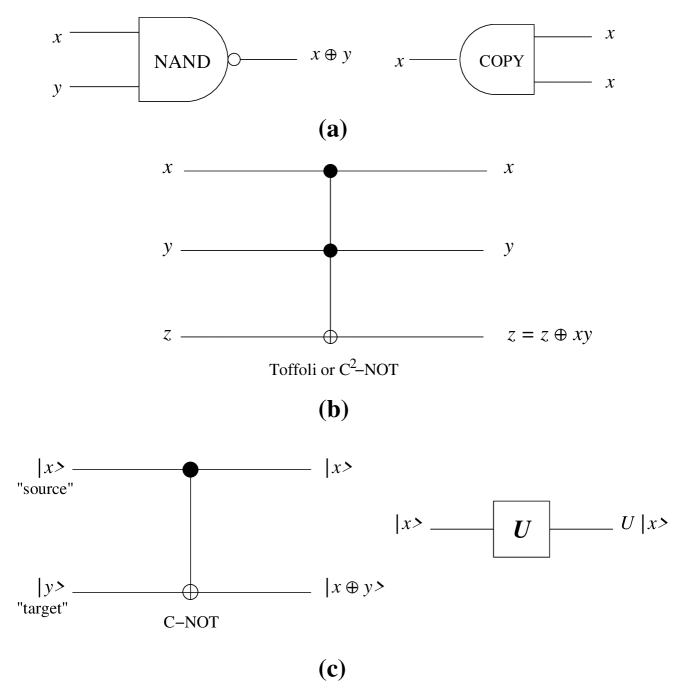
Figure 3.4: Gates for universal computation: (a) for irreversible classical computation (b) for reversible classical computation (c) for quantum computation.

In these diagrams, the bits being operated on “travel” from left to right through the gate, and have an effect described by the outputs; for instance if the Boolean values $x=1$ and $y=1$ are input into a NAND gate, the output will be $x\oplus y=1\oplus 1=0$. Other sets of gates are also universal. For classical reversible computation, the three-input Toffoli gate is universal. This gate is also called a “controlled-controlled-NOT” (C²-NOT), since the “target” bit is negated if and only if the two “source” bits are both 1; otherwise the target bit is untouched.

In quantum computing we are no longer dealing with abstract Boolean values, but with two-level quantum states whose states we denote $|0\rangle$ and $|1\rangle$. Note that mathematically, any Hilbert space can be considered as a subspace of the joint space of a set of qubits, so by considering operations on qubits we are not losing any generality. The most general quantum evolution is unitary, so the question is: What type of qubit operations are required to implement an arbitrary unitary operator on their state space? Deutsch [95] provided an answer: all we need is a “controlled-controlled-$R$”, where $R$ is any qubit rotation by an irrational fraction. A more convenient set [99] is that shown in Figure 3.4(c), the set comprising the C-NOT and arbitrary single qubit rotations (such rotations are elements of $U(2)$ and can be represented by four real parameters). And interestingly, any single unitary operation acting on two or more qubits is generically universal [100]. While this is a mathematically simple remark, physically this means that any unitary operation in $d$ dimensions can be carried out using a single fixed “local” rotation — where by local we mean “operating in exactly four dimensions” (two qubits).

The reader may object that certain gate sets will be more practical than others; in particular, attempting to compute using just one two-qubit gate looks like an uphill battle compared with, say, using the gate set shown in Figure 3.4(c). However, the issue of complexity is implicit in the definition of “universal”: a gate set is only universal if it can simulate any other gate set with polynomial slowdown; indeed, in the analysis of any proposed quantum algorithm, the complexity of the required gates must be taken into account. Such issues are addressed in e.g. [95], [99].

The answer to the final question posed above is difficult, and is related to the open problem in computing theory of classifying problems into complexity classes. Not all classically exponential-time problems can be reduced to polynomial-time on a quantum computer — in fact there appear to be very few of these, although many problems admit a square-root or polynomial speed-up. General mathematical frameworks for the quantum factorisation problem are given by Mosca and Ekert [101] and for the quantum searching problem by Mosca [102]. The relation of current quantum algorithms (in the network model mentioned above) to the paradigm of multi-particle interferometry is given by Cleve et al [103].

3.4 Quantum Channels

The idea of a quantum channel was implicit in the discussion of quantum noiseless coding: the channel consisted of Alice sending Bob a “coded” physical system through an effectively noiseless channel. This is an idealisation; any means that Alice and Bob share for transmitting information is subject to imperfection and noise, so we should analyse how this noise can be characterised and whether transmission of intact quantum states can be achieved in the presence of noise. Ideally we would like to arrive at a “quantum noisy coding theorem”.

Note that, just as in the classical case, error correction in quantum channels is not solely important for the obvious task of Alice sending information to Bob. Coding techniques are also used to protect information which is “transmitted” through time — as for example the data stored in computer memory, which is constantly refreshed and checked using parity codes. If we are to implement useful quantum computations, we will need similar coding techniques to prevent the decoherence (loss into the environment) of the quantum information.

It is instructive to look first at how classical communication and computation are protected against errors. In general the “imperfection and noise” can be well characterised by a stochastic process acting on the information, whose effect is to flip signal $i$ to signal $j$ with probability $p(j|i)$. We can remove the errors through mathematical or physical techniques; by using redundancy or by engineering the system to be insensitive to noise. This insensitivity is a result of combining amplification with dissipation [104]: the amplification provides a “restoring force” on the system, while dissipation causes oscillations away from equilibrium to be damped. This is the primary source of reliability in a modern classical computer. Unfortunately, it is precisely these types of robustness which are not available in quantum systems; we cannot amplify the state by copying it, and we cannot subject it to dissipative (non-unitary) evolutions.

What about redundancy? This plays a more important role in classical communication than in computing. Error-correcting codes — a vast subject of research in itself [105] — were at first thought to be inapplicable to quantum systems for the same reason that amplification is not allowed. However, once it was realised that redundancy could be achieved by encoding the state of a qubit into a much larger space (say that of five qubits) which is more robust against decoherence, the techniques of classical coding theory could be used to discover which subspaces should be used. A quantum theory of error correction has thus grown with techniques parallel to the classical theory, as will be discussed in Section 3.4.2.

3.4.1 Entanglement Purification

One way to transmit quantum information is to teleport it. In a certain sense this is a circular argument, because for teleportation Alice and Bob require shared entanglement — a resource which requires transmission of coherent quantum information in the first place. Fortunately, Bennett et al have had a word with Alice and Bob and told them how to go about getting almost pure Bell states out of a noisy channel [47].

Before we discuss this, we need to know what operations are available to Alice and Bob. It turns out that all we will need for this entanglement purification protocol (EPP) is three types of operations: (i) unilateral rotations by Alice using the operators $\sigma_{x},\sigma_{y},\sigma_{z}$; (ii) bilateral rotations, represented by $B_{x},B_{y},B_{z}$ which represent Alice and Bob both performing the same rotation on their qubits; and (iii) a bilateral C-NOT, where Alice and Bob both perform the operation C-NOT shown in Figure 3.4(c), where both the members of one pair are used as source qubits and both qubits from another pair are used as target qubits. The effects of these operations are summarised in the table in Figure 3.5 (complex phases are ignored in this table).

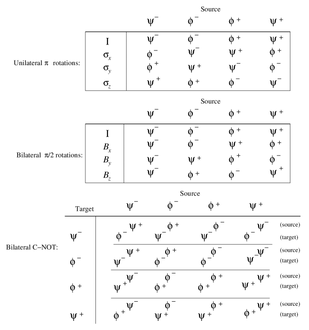
Figure 3.5: The unilateral and bilateral operations used in entanglement purification (after [47]).

For example, if Alice and Bob hold a pair $AB$ of qubits in the state $|\phi^{+}\rangle$ and either Alice or Bob (but not both) perform the unitary operation $\sigma_{y}$ on their half of the pair, they have performed a unilateral $\pi$ rotation. According to the table, pair $AB$ will now be described by the state $|\psi^{-}\rangle$. If they had both performed the same $\sigma_{y}$ operation on their respective qubits (a bilateral $B_{y}$ operation) then we see from the tabel that the state of $AB$ would remain $|\phi^{+}\rangle$.

Note how the bilateral C-NOT is implemented: Alice prepares systems $AB$ and $CD$ in Bell states, and sends $B$ and $D$ to Bob. Bob uses $B$ as source and $D$ as target in executing a C-NOT, while Alice uses $A$ as source and $C$ as target (this is illustrated in Figure 3.6). In general, both pairs $AB$ and $CD$ will end up altered, as shown in the table in Figure 3.5. For example, if the source pair $AB$ is prepared as $|\psi^{+}\rangle$ and the target pair $CD$ as $|\phi^{+}\rangle$, then we conclude from the table that after this operation the pair $AB$ remains in the state $|\psi^{+}\rangle$, but the pair $CD$ is now described by $|\psi^{+}\rangle$ as well.

The most general possible way of describing the noise is as a superoperator $\$$ acting on the transmitted states. We suppose that Alice manufactured a large number of pairs of systems in the joint state $|\psi^{-}\rangle$, and when she sent half of them through the channel to Bob they were corrupted by the joint superoperator $\leavevmode\hbox{\small 1\kern-3.8pt\normalsize 1}\otimes\$$ (Alice preserves her half perfectly). We are only interested in the state $\rho_{AB}$ which emerges. This matrix, expressed in the Bell basis, has three parts which behave differently under rotation: the $|\psi^{-}\rangle\langle\psi^{-}|$ behaves as a scalar, 3 terms of the form $|\psi^{-}\rangle\langle\nu|$ ($|\nu\rangle$ is one of the Bell states) which behave as a vector, and the $3\times 3$ block which behaves as a second rank tensor. Bennett et al showed that through a random operation of twirling any state $\rho_{AB}$ can be brought into the so-called Werner form:

$$W_{F}=F|\phi^{+}\rangle\langle\phi^{+}|+\frac{1-F}{3}\left(|\psi^{+}\rangle\langle\psi^{+}|+|\psi^{-}\rangle\langle\psi^{-}|+|\phi^{-}\rangle\langle\phi^{-}|\right).$$ (3.30)

This “twirling” is done by performing a type of averaging: for each EPR pair she generates, Alice chooses randomly one element from a set of specially chosen combinations of the operations $B_{x},B_{y},B_{z}$, tells Bob which one it is, and they perform the specified operation. The “twirls” are chosen so that the second rank tensor representing the states, when acted upon by these random twirls, becomes proportional to the identity and the vector components disappear. The idea is similar to motional averaging over the directional properties of a fluid, where all vector quantities are zero and tensor properties can be described by a single parameter.

Alice and Bob can now consider their ensemble of EPR pairs as a classical mixture of Bell states, with proportion $F$ of the state $|\phi^{+}\rangle$ and $\frac{1-F}{3}$ of each of the other states. This is enormously useful because they can employ classical error correction techniques to project out and find pure singlet states. There is a price paid, though: we have introduced additional uncertainty, and this is reflected by the fact that $S(W_{F})>S(\rho_{AB})$. It can be shown that the protocol described below works without the twirl, but this is a more subtle argument. Note that $F$ is the fidelity between the Werner state and the state $|\phi^{+}\rangle$: $F=\langle\phi^{+}|W_{F}|\phi^{+}\rangle$, where the fidelity of a transmitted state was defined in Eqn 2.64.

After this pre-processing stage, Alice and Bob perform the following steps:

1. They select the corresponding members of two pairs from their ensemble.

2. They perform a bilateral C-NOT from the one pair to the other (illustrated in Figure 3.6).

3. They make (local) measurements on the target pair to determine its amplitude bit.

4. If the amplitude bit is 1 (i.e. if the target pair is in one of the $\phi$ states) then both pairs are discarded. If the amplitude bit is 0, which occurs with probability $p_{\rm pass}=F^{2}+\frac{2}{3}F(1-F)+\frac{5}{9}(1-F)^{2}$, the source pair is in the state $W_{F^{\prime}}$ with

   $$F^{\prime}=\frac{F^{2}+\frac{1}{9}(1-F)^{2}}{F^{2}+\frac{2}{3}F(1-F)+\frac{5}{9}(1-F)^{2}}$$ (3.31)

   Proof of this relation is left as an exercise for the reader, using the information from Figure 3.5 and Eqn 3.30.

                 

Figure 3.6: An illustration of the bilateral C-NOT operation, and its effect on the fidelity of the Werner state (taken from [47]).

How exactly does this help us? Well the answer is shown in Figure 3.6: for all starting fidelities $F>1/2$, we have that $F^{\prime}>F$. So with probability of success $p_{\rm pass}\leq 1/2$ we will have succeeded in driving the Werner state closer to a pure Bell state.

We may want to know how many EPR pairs $m$ can be distilled from $n$ copies of the intial state $\rho_{AB}$ as $n$ gets large; that is, we define the yield of a protocol $P$ to be

$$D_{P}(\rho_{AB})=\lim_{n\rightarrow\infty}m/n.$$ (3.32)

Unfortunately the yield of this protocol is zero. At each step we are throwing away at least half of our pairs, so this process is very wasteful. However, this protocol can be used in combination with other protocols to give a positive yield. In particular, Bennett et al [47] describe a variation of a classical hashing protocol which gives good results.

An important feature to note about these protocols is that they explicitly require two-way communication between Alice and Bob, and so we may call them 2-EPP. What about 1-EPP — those protocols which use only communication in one direction? There is certainly an important distinction here. 1-EPP protocols can be used to purify entanglement through time, and thus to teleport information forward in time. This is exactly what one wishes to achieve using quantum error-correcting codes (QECC). On the other hand, a 2-EPP can be used for communication but not for error-correction. In fact, we can define two different rates of communication using EPP, for a particular channel desribed by superoperator $\$$:

$$D_{1}(\$) = \sup_{\mbox{\scriptsize P is a 1-EPP}}D_{P}(\rho_{AB})$$ (3.33)

$$D_{2}(\$) = \sup_{\mbox{\scriptsize P is a 2-EPP}}D_{P}(\rho_{AB}).$$ (3.34)

(Note that one EPR pair allows perfect transmission of one qubit, using teleportation; hence the number of Bell states distilled can be interpreted as a rate of transmission of quantum information.) Clearly, since all 1-EPP are also 2-EPP, we have $D_{2}\geq D_{1}$. It can be shown that for some mixed states $\rho_{AB}$ — or equivalently, for some channels $\$$ — there is a strict separation between $D_{1}$ and $D_{2}$; in fact there are some mixed states with $D_{1}=0$ and $D_{2}>0$ [47].

We can see now the importance of the entanglement swapping protocol presented earlier. For most quantum communication channels, the fidelity is an exponentially decreasing function of distance $l$. Ususally this is described by a coherence length $l_{0}$. However if we divide the length $l$ into $N$ intervals, the fidelity change over each interval is $\exp(-l/Nl_{0})$, which can be made as close to unity as required. Using EPP we can improve the fidelity over each interval as much as required and then perform the entanglement swapping protocol approximately $\log_{2}N$ times to achieve high fidelity entanglement between the beginning and end points [107]. Using this technique, the fidelity can be made into a polynomially decreasing function of distance, which shows that is is possible in principle for us to implement long-distance quantum communication.

Two other EPPs worth noting are the Procrustean method and the Schmidt projection method [106] — although this more for their historical interest. They are both designed to operate on non-maximally entangled pure states.

3.4.2 Quantum Error Correction

At first sight, quantum errors don’t seem amenable to correction — at least not in a similar sense to that of classical information. Firstly, quantum information cannot be copied to make it redundant. Secondly, quantum errors are analogue (as opposed to digital) errors: it can make an enormous difference if the state $a|0\rangle+b|1\rangle$ is received as $(a+\epsilon_{1})|0\rangle+(b-\epsilon_{2})|1\rangle$, whereas in classical error correction we just need to prevent a system in the state ‘0’ from entering the state ‘1’ and vice versa.

The first problem is countered by using logical states, which correspond to the $|0\rangle$ and $|1\rangle$ states of a two-level system, but which are in fact states of a much larger quantum system. In effect, we can use $n$ qubits with a $2^{n}$-dimensional Hilbert space, but only employ two states $|0_{L}\rangle$ and $|1_{L}\rangle$ in communication. We aim to design these states so that $a|0_{L}\rangle+b|1_{L}\rangle$ is recoverable despite errors.

The second problem is solved by realising that errors can be digitised. Suppose we make a measurement onto our redundant system, and we choose our POVM to be highly degenerate, so that the only information it yields is which subspace the system is in. If we choose our redundancy carefully, and make a well-chosen measurement, we will project (and so discretise) the error and the measurement result will tell us which error has occurred in this projected system. This will be elaborated below, after we have discussed the type of errors we are dealing with.

As mentioned previously errors are introduced through interaction with the environment, which can be represented by the action of a superoperator on the state we are transmitting. Rather than using the operator-sum representation we will explicitly include the environment in our system — and we lose no generality in representing a superoperator if we assume that the environment starts out in a pure state $|e_{0}\rangle$. Then the state of the code system which starts as $|\phi\rangle$ will evolve as

$$|e_{0}\rangle|\phi\rangle\longrightarrow\sum_{k}|e_{k}\rangle S_{k}|\phi\rangle$$ (3.35)

where the $S_{k}$ are unitary operators and the $|e_{k}\rangle$ are states of the environment which are not necessarily orthogonal or normalised. The $S_{k}$ are operators on the code system Hilbert space, and form a complex vector space; so we choose some convenient basis for the space consisting of operators $M_{s}$:

$$S_{k}=\sum_{s}a_{ks}M_{s}$$ (3.36)

where $a_{sk}$ are complex constants. If we define $|e_{s}^{\prime}\rangle=\sum_{k}a_{ks}|e_{k}\rangle$, then the final state of the system+environment in Eqn 3.35 will be $\sum_{s}|e_{s}^{\prime}\rangle M_{s}|\phi\rangle$. Once again the environment state vectors are not orthogonal or normalised, but we can now choose the operators $M_{s}$ to have convenient properties.

We note first of all that not all the errors can be corrected. This follows because not all the states $M_{s}|\phi\rangle$ can be orthonormal, so we cannot unambiguously distinguish between them to correct $M_{s}$. So we do the next best thing: we choose a certain subset $\cal M$ (called the correctable errors) of the operators $M_{s}$ and seek to be able to correct just these errors.

What do we mean by “correcting errors”? Errors will be corrected by a recovery operator: a unitary operator $\cal R$ which has the following effect:

$$\mbox{$\cal R$}|\alpha\rangle M_{s}|\phi\rangle=|\alpha_{s}\rangle|\phi\rangle$$ (3.37)

where $|\alpha\rangle$ and $|\alpha_{s}\rangle$ are states of everything else (environment, ancilla, measuring apparatus) and $M_{s}$ is any correctable error. In general the states $|\alpha_{s}\rangle$ are not going to be orthogonal, but the important feature is that the final state $|\phi\rangle$ of the code system must not depend on $|\alpha_{s}\rangle$ — if it did depend on the code system state then error recovery would not work on linear combinations of states on which it does work, so universal error correction would be impossible.

A quantum error-correcting code (QECC) is a subspace $V$ of the $2^{n}$-dimensional space describing $n$ qubits together with a recovery operator $\cal R$. This QECC must satisfy the following conditions: for every pair of code words $|u\rangle,|v\rangle\in V$ with $\langle u|v\rangle=0$ and every pair of correctable errors $M_{s},M_{t}\in\mbox{$\cal M$}$,

$$\langle u|M_{s}^{\dagger}M_{t}|v\rangle = 0$$ (3.38)

$$\langle u|M_{s}^{\dagger}M_{t}|u\rangle = \langle\alpha_{s}|\alpha_{t}\rangle$$ (3.39)

with Eqn 3.39 holding independent of the code word $|u\rangle$. These conditions imply that errors can be corrected, as can be seen in the following way. For any code words the recovery operator acts as

$$\mbox{$\cal R$}|\alpha\rangle M_{s}|u\rangle=|\alpha_{s}\rangle|u\rangle\hskip 28.45274pt\mbox{$\cal R$}|\alpha\rangle M_{t}|v\rangle=|\alpha_{s}\rangle|v\rangle.$$ (3.40)

Taking the inner product on both sides between these we find that

$$\langle u|M_{s}^{\dagger}\langle\alpha|\mbox{$\cal R$}^{\dagger}\mbox{$\cal R$}|\alpha\rangle M_{t}|v\rangle = \langle\alpha_{s}|\alpha_{t}\rangle\langle u|v\rangle$$ (3.41)

$$\Rightarrow\langle u|M_{s}^{\dagger}\langle\alpha|\alpha\rangle M_{t}|v\rangle = \langle\alpha_{s}|\alpha_{t}\rangle\delta_{uv}$$ (3.42)

where $\mbox{$\cal R$}^{\dagger}\mbox{$\cal R$}=\leavevmode\hbox{\small 1\kern-3.8pt\normalsize 1}$ since $\cal R$ is unitary. The requirements listed above follow if $\langle u|v\rangle=0$ or $u=v$ respectvely.

By reversing the above arguments, we find that Eqs 3.38 and 3.39 are also sufficient for the existence of a QECC correcting errors $\cal M$. The aim in designing QECC’s is thus to identify the most important or likely errors acting on $n$ qubits, identify a subspace which satisfies the requirements above, and find the recovery operator. This can be a complex task, but fortunately many of the techniques of classical coding theory can be brought to bear. We will briefly sketch the most common ideas behind classical error correction and indicate how these ideas may be modified for QECC.

The simplest error model in classical coding theory is the binary symmetric channel. Binary refers to the fact that two signals are used, and symmetric indicates that errors affect both signals in the same way, by flipping $0\!\leftrightarrow\!1$; in addition, we assume that the errors are stochastic i.e. affect each signal independently and with probability $p$. In this case we can apply the algebraic coding techniques pioneered by Hamming [105] to design parity check codes. The classical result is that, by using a $k$ bit ($2^{k}$-dimensional) subspace of words of length $n$ (with $k<n$), we can design a code that corrects up to $t$ errors; the Hamming bound on linear codes is

$$k\leq n-\log_{2}\sum_{i=0}^{t}\big{(}\!\begin{array}[]{c}n\\[-5.69054pt] i\end{array}\!\big{)}$$ (3.43)

where the term inside the sum is the binomial coefficient. Essentially the sum in this expression counts the number of different ways in which up to $t$ errors can occur, and this is a lower bound to the number $n-k$ of redundant bits required for error correction.

Similar algebraic techniques can be applied to a quantum generalisation of the binary symmetric channel. In this case we take as a basis for the errors the qubit operators $I=\leavevmode\hbox{\small 1\kern-3.8pt\normalsize 1},X=\sigma_{x}$, $Y=-i\sigma_{y}$ and $Z=\sigma_{z}$ (we have introduced a factor of $-i$ into $Y$ for convenience); explicitly,

$$I=\left(\begin{array}[]{cc}1&0\\ 0&1\end{array}\right)\hskip 28.45274ptX=\left(\begin{array}[]{cc}0&1\\ 1&0\end{array}\right)\hskip 28.45274ptY=\left(\begin{array}[]{cc}0&-1\\ 1&0\end{array}\right)\hskip 28.45274ptZ=\left(\begin{array}[]{cc}1&0\\ 0&-1\end{array}\right).$$ (3.44)

These operators correspond to a bit flip $0\!\leftrightarrow\!1$ ($X$), a phase flip $0\!\rightarrow\!0,1\!\rightarrow\!-1$ ($Z$) or both ($Y=XZ$) — a much richer set of errors than in the classical case! We will use a system of $n$ qubits, so a typical error will be $M_{s}=I_{1}X_{2}Z_{3}\ldots Y_{n-1}I_{n}$. In analogy with the classical case, a sensible choice of correctable errors will be those with weight $\leq t$, where the weight is the number of single qubit error operators which are not $I$ — although if we have more sophisticated knowledge of the noise, such as correlations between qubits, we would hope to include these as well. For example, a single error-correcting QECC can be constructed using 5 qubits, to be compared with a classical single error-correcting code which uses 3 bits (it only corrects $X$ errors) [22].

An interesting feature to note about a $t$-error correcting QECC is that the information is encoded highly nonlocally. For example, suppose we have encoded a single qubit into 5 qubits using the optimal 1-error correcting code. If we handed any one qubit over to an eavesdropper Eve, then the fidelity of our quantum system after recovery can still be arbitrarily high — and so by the no-cloning theorem Eve will not have been able to derive any information from her qubit. Contrast this with the classical case, in which, if Eve knew that the probability of error on any single qubit was $p\ll 1$, she could be confident that the signal was what she measured. In fact, if in the course of recovery we make a measurement (as will usually be the case; the operator $\cal R$ above includes this possibility) on the qubits, the result cannot reveal any information about the logical state encoded in the set of qubits, for otherwise we will have disturbed the quantum information. These are important features of quantum error correction.

A pedagogical survey of QECC and coding techniques can be found in [22], and a good set of references is given in the appropriate section of [104].

Quantum channel capacity

So where does all of this leave us in terms of channel capacity? Our aim would be to characterise the number of qubits which can be recovered after the action of a superoperator $\$$ with arbitrarily good fidelity.

The quantum version of the problem of channel capacity is mathematically a great deal more complicated than the classical version, so we would expect an answer to this question to be more difficult to reach. But we are faced with even more complication: the capacity depends on what other resources are available. For example, there are channels which cannot be used to communicate quantum states if only one-way communication is allowed, but have positive capacity if two-way communication is allowed [47]. On the other hand, $t$-error correcting QECCs exist with an asymptotic rate $k/n=1-2H(2t/n)$ [108], where $H$ is the entropy function — so if the errors are uncorrelated and have low enough average probability on each single qubit, we can transmit quantum information with arbitrarily good fidelity. The Shannon strategy of random coding is found to fail when transplanted into quantum information terms. Altogether, there are very few answers to the general characterisation of quantum channel capacity.

Fault tolerant quantum computing

Another, possibly fatal, criticism can be found for quantum error correction ideas. A QECC uses extra qubits to encode one qubit of information, and requires us to “smear” the information over these other systems. This will require interaction between the qubits, and such interaction will in general be noisy; and extra qubits mean that each qubit has the potential to interact with the environment — noise which can spread through interactions between qubits. So the burning question is: Can we, by introducing more qubits and more imperfect interactions, extend a computation? Can we decrease the logical error rate?

This is a serious problem, which initially seemed like a death blow to implementing quantum computing even in principle. However, careful analysis has shown that coherent quantum states can be maintained indefinitely, despite imperfect gates and noisy qubits, as long as the error rate is below a certain threshhold. Such analyses are the subject of the enormous field of fault tolerant quantum computing. Further discussion of this topic can be found in [109].

3.5 Measures of Entanglement

With some idea of what entanglement can be used for and how to interchange forms of entanglement, we can return to the problem of quantifying an amount of entanglement.

We can immediately define two types of entanglement for any bipartite quantum state $\rho_{AB}$: the entanglement of formation $E_{F}$, which is the minimum number of singlet states $|\psi^{-}\rangle$ required to prepare $\rho_{AB}$ using only local operations and classical communication (LOCC); and the entanglement of distillation $E_{D}$, which we define to be the maximum number of EPR pairs which can be distilled from $\rho_{AB}$ — with the maximum taken over all EPPs.

Bennett et al [47] showed the very useful result that for pure states $|\psi_{AB}\rangle$ of the joint system, the following result holds:

$$E_{F}=E(|\psi_{AB}\rangle)=E_{D}$$ (3.45)

where $E(\cdot)$ is the entanglement measure proposed earlier in Eqn 3.18. The first equality follows from the fact that Alice can locally create copies of $|\psi_{AB}\rangle$, compress them using Schumacher coding, and teleport the resulting states to Bob who can uncompress them; the second equality can be shown to hold by demonstrating an EPP which achieves this yield. This is the sense, alluded to previously, in which a single system in the state $|\psi_{AB}\rangle$ can be thought of as equivalent to $E$ singlet states. This relation immediately allows us to simplify the definition of $E_{F}$ for mixed states. If we denote by ${\cal E}_{\rho}=\{|\psi^{i}_{AB}\rangle;p_{i}\}$ an ensemble of pure states whose density operator is $\rho$, then the entanglement of formation of $\rho$ is

$$E_{F}(\rho)=\min_{{\cal E}_{\rho}}\sum E(|\psi^{i}_{AB}\rangle).$$ (3.46)

This is justified by the fact that if we have $E_{F}(\rho)$ singlets, then Alice can teleport a probabilistic mixture of pure states to Bob to end up with the density operator $\rho$. Wootters [110] has derived an exact expression for the entanglement of formation of any state of two qubits.

Notice that in general $E_{F}\geq E_{D}$, since if this were otherwise, we could form an entangled state from $E_{F}$ EPR pairs and distill a greater number of EPR pairs from that! Evidence suggests [47] that the inequality is strict for all mixed states over the joint system.

Recall the definition in Eqn 3.20 of a separable bipartite state. We might ask whether there is any way to determine whether a state is mixed without laboriously writing it in this form; and we would be stuck for an answer.

Firstly, we might suppose that such states would always exhibit nonlocal correlations such as in Bell’s inequalities. This attempt fails because there are mixed states (in fact, the Werner states introduced earlier) which do not violate any Bell’s inequality because they admit hidden variables descriptions [111]. Indeed, there are separable states which have nonlocal properties; Bennett et al [87] demonstrated a set of bipartite states of two 3-state systems which can be prepared locally but which cannot be unambiguously discriminated by local measurements.

Secondly, we could ask whether all non-separable states can be used for something like teleportation — since the Werner states can indeed be used for this [112]. We would once again encounter a blind alley, since there are states which are nonlocal but cannot be used in quantum teleportation [113]. This entanglement is termed “bound”, in analogy with bound energy in thermodynamics which cannot be used to do useful work — this entanglement cannot perform any useful informational work.

Note that if a state can be used for teleportation, it can be purified to singlet form (by Alice teleporting singlets to Bob). Obviously, if a state can be distilled then it can be used for teleportation; so there is an equivalence here.

In the spirit of trying to figure out what entanglement means, DiVincenzo et al suggested another measure of entanglement, the entanglement of assistance [60]. It is defined very similarly to entanglement of formation:

$$E_{A}(\rho)=\max_{{\cal E}_{\rho}}\sum E(|\psi^{i}_{AB}\rangle).$$ (3.47)

Obviously this function will have properties dual to those of $E_{F}$. It has some expected properties — such as non-increase under LOCC — but some unexpected features too. $E_{A}$ also has an interpretation in terms of how much pure state bipartite entanglement can be derived from a tripartite state. And Vedral et al [114] have found a whole class of entanglement measures based on quantifying the distance of a state from separability.

There is still much room for new ideas in quantifying of entanglement, and in finding uses for it — qualifying entanglement. In a certain sense entanglement is a “super” classical correlation: it holds the potential for classical correlation, but that potential is only realised when a measurement is made. On the other hand it is also a very simple concept: it represents the fact that systems do not exist in classically separated states. Entanglement is merely a manifestation of this unity.

Chapter 4 Conclusion

David Mermin [115] once identified three post-quantum theory generations of physicists according to their views on the quantum. The first, who were around when the theory developed (which includes the “Founding Fathers”), were forced to grapple with the elements of the theory to give it a useful interpretation. Once a workable theory was developed, however, this generation came to regard the quirks of quantum theory as due to some deeply ingrained “classical” modes of thought and hence to be expected. The second generation — their students — took this lesson further by insisting that there was nothing unusual about quantum mechanics, and tried to make it mundane; and indeed, this “shut-up-and-calculate” approach did yield fruitful developments. The third generation, of which Mermin claims membership, doesn’t seem to have much of an opinion one way or the other, regarding the theory as productive and empirical and carrying on. But, Mermin points out, when foundational questions are raised, the reaction of this generation varies from irritated to bored to plain uncomfortable.

To this we can now add another generation: those with enough familiarity with the more bizarre parts of the theory not to be blasé about it, but who take a practical approach by asking: What’s so special about this theory? How can we characterise it? If a classical ontology for this theory doesn’t work — if billiard balls and elastic collisions don’t describe the microscopic world — then what can be wrought from quantum theory in their place?

One famous illustration of this attitude — albeit from a member of the third generation — is the EPR paradox and its resolution by Bell. Bohr’s own response to the EPR paper had been guarded and had appealed to his own orthodox interpretation; in a way the EPR dilemma was likened to counting angels on the head of a pin. The strongest argument against EPR was that mutually contradictory experimental setups should not be compared. But with a more pragmatic approach, Bell succeeded in eschewing metaphysical arguments in favour of contemplation of the theory and reasoning of the first class. This is a valuable lesson which has not gone unlearned in the field of information physics. Since quantum physics is an inherently statistical theory, we cannot properly engage with it without considering what those statistics mean in the real world — both as input and as output from the theory. How do we operationally define a quantum state? How much error do we introduce in our preparation, and how much is intrinsic according to the theory? These are some of the questions which information physics has addressed.

Some of the current concerns of quantum information physics have been described in this thesis. The compression of mixed states is a minefield, but the curious examples cited in [74] illustrate that much work is still to be done in the mapping of this minefield. The quantification of entanglement, classification of qualitatively different types of entanglement, their interconvertibility and their purification are still major focuses of work in quantum information theory.

The implications of information physics reach further than questions of compression and capacity. An obvious application of this study is to high-precision measurement and to feedback control of quantum systems. The third generation of gravitational wave detectors for the LIGO experiment is expected to achieve a sensitivity beyond the standard quantum limit for position monitoring of a free mass [12], and novel techniques for measurement will have to be found. For example, we could consider the Hamiltonian $H(x)$ of the mass to be controlled by a parameter $x$, and it is our task to determine $x$ from measurements on the mass. In this case we can consider the resulting state of the mass (after evolution for a time $t$) to be one of a set of states $\rho_{x}$. How much information about $x$ can be extracted from this ensemble? And what is the optimal measurement? These are questions addressed by theorems presented here as well as in ongoing research into techniques for optimal extraction of information. An illustration of the insight afforded by quantum information theory is the following: suppose two electrons are in pure states with their spin polarisation vectors both pointing along the same unknown axis but possibly in different directions. Then more information about this unknown direction can be extracted from the pair of electrons if they are anti-parallel rather than parallel [116].

Indeed, ideas from quantum computing can also be of assistance in this. Grover’s search algorithm was proposed to find some input $x$ to a “black box” binary-valued function $f$ such that the output is 1: $f(x)=1$. Essentially what is achieved through this algorithm is the extraction of global information about the black box Hamiltonian through our addition of controlled terms to this Hamiltonian [12]. Hence through quantum algorithm analysis we can find an optimal driving to apply to our measurement system and the measurement to apply in order to characterise the unknown Hamiltonian affecting our LIGO III detector.

Characterisation of entanglement and information in quantum systems is also important in studying quantum chaos [117]. In these cases it becomes important to specify our information about a chaotic system and how it behaves under small perturbations. This leads us to introduce the concept of algorithmic entropy [118], which is a spin-off of classical computing theory and accurately captures the idea of “complexity” of a system.

Much current work in information theory is aimed at narrowing the gap between the theory described in this thesis and available experimental techniques. Quantum computing is a major focus of these efforts, with a great deal of ingenuity being thrown at the problem of preserving fragile quantum states. Quantum error correction and fault-tolerant quantum computing are two of the products of such efforts, and further analysis of particular quantum gates and particular computations is proceeding apace. A recent suggestion to simplify a prospective “desk-top” quantum computer involves supplying ready-made generic quantum states to users who thus require slightly less sophisticated and costly hardware [69]; hence quantum computing may ultimately also depend on faithful communication of quantum states.

And of course, the million-dollar question in quantum computing is: What else can we do with a quantum computer? Factoring large integers is a nice parlour trick and will enable a user to crack most encryption protocols currently used on the internet. But is this enough of a reason to try and build one — particularly considering that in the near future quantum key distribution may become the cryptographic protocol of choice? Also, while Grover’s search algorithm gives a handsome speed-up over classical search techniques (and some computer scientists are already designing quantum data structures), it will be a long time before Telkom starts offering us quantum phone directories.

There is something for the romantics in quantum information theory too — at least those romantics with a taste for foundational physics. The following quote (from [12]) is rather a dramatic denunciation of quantum computer theorists:

It will never be possible to construct a ‘quantum computer’ that can factor a large number faster, and within a smaller region of space, than a classical machine would do, if the latter could be built out of parts at least as large and as slow as the Planckian dimension.

This statement comes from Nobel laureate Gerard ’t Hooft. Are we missing something from quantum mechanics? Will quantum mechanics break down, perhaps at the Planck scale? An interesting observation of fault-tolerant quantum computing is that the overall behaviour of well-designed circuit can be unitary for macroscopic periods of time — perhaps using concatenated coding [109] — despite almost instantaneous decoherence and non-unitary behaviour at a lower level. Is nature fault-tolerant? Rather than constructing a solar system-sized particle accelerator, we would be well-advised to assemble a quantum computer and put the theory through its paces in the laboratory.

On the other hand, we may be able to deduce, à la Wootters [39], some principles governing quantum mechanics — information-theoretic principles, which constrain the outcomes of our proddings of the world. Weinberg, after failed attempts to formulate testable alternatives to quantum mechanics, suggested [12]:

This theoretical failure to find a plausible alternative to quantum mechanics suggests to me that quantum mechanics is the way it is because any small changes in quantum mechanics would lead to absurdities.

It’s been a century since the discovery of the quantum: what lies in store in the next 100 years?

REFERENCES

References

- [1] D. Deutsch, A. Ekert and R. Lupacchini, “Machines, logic and quantum physics,” arXiv:math.HO/9911150.
- [2] J. A. Rice, Mathematical Statistics and Data Analysis. New York: Wadsworth, 1994.
- [3] J. C. Taylor, An introduction to measure and probability. New York: Springer, 1997.
- [4] C. R. Smith and G. Erickson, “From rationality and consistency to Bayesian probability,” in Maximum Entropy and Bayesian Methods, Cambridge, U.K., 1988 (J. Skilling ed.). Dordrecht: Kluwer, 1988.
- [5] R. T. Cox, “Probability, frequency, and reasonable expectation,” American Journal of Physics, Vol. 14(1), pp. 1-13 (1946).
- [6] A. Peres, Quantum Theory: Concepts and Methods. Dordrecht: Kluwer, 1993.
- [7] D. A. Lane, “Fisher, Jeffreys, and the nature of probability,” in R. A. Fisher: An Appreciation (S. Feinberg et al, eds.). New York: Springer-Verlag, 1980.
- [8] T. M. Cover and J. A. Thomas, Elements of Information Theory. New York: John Wiley & Sons, 1991.
- [9] C. E. Shannon, “The mathematical theory of communication,” in C. E. Shannon and W. Weaver, The Mathematical Theory of Communication. Urbana: University of Illinois Press, 1949.
- [10] J. Aczél and Z. Daróczy, On Measures of Information and Their Characterizations. New York: Academic Press, 1975.
- [11] R. Schack and C. M. Caves, “Classical model for bulk-ensemble NMR quantum computation,” Physical Review A, Vol. 60(6), pp. 4354-4362 (1999). arXiv:quant-ph/9903101.
- [12] J. Preskill, “The future of quantum information science,” talk at the NSF Worshop on Quantum Information Science (28 October 1999). Available at http://www.theory.caltech.edu/people/preskill/ph229.
- [13] C. A. Fuchs, “The Structure of Quantum Information,” unpublished paper.
- [14] C. M. Caves, C. A. Fuchs, “Quantum information: How much information in a state vector?” in Sixty Years of EPR (A. Mann and M. Revzen, eds.). Israel: Ann. Phys. Soc., 1996. arXiv:quant-ph/9601025.
- [15] W. K. Wootters, “Random quantum states,” Foundations of Physics, Vol. 20(11), pp. 1365-1378 (1990).
- [16] B. Schumacher, “Sending entanglement through noisy channels,” Physical Review A, Vol. 54(4), pp. 2614-2628 (1996). arXiv:quant-ph/9604023.
- [17] J. Eisert, M. Wilkens and M. Lewenstein, “Quantum games and quantum strategies,” Physical Review Letters, Vol 83(15), pp. 3077-3080 (1999). arXiv:quant-ph/9806088.
- [18] B. Schumacher, “Quantum Coding,” Physical Review A, Vol. 51(4), pp. 2738-2747 (1995).
- [19] W. K. Wootters, “Statistical distance and Hilbert space,” Physical Review D, Vol. 23(), pp. 357-362 (1981).
- [20] E. H. Lieb and J. Yngvason, “A fresh look at entropy and the second law of thermodynamics,” Physics Today, pp. 32-37 (April 2000)
- [21] A. Wehrl, “General properties of entropy,” Reviews of Modern Physics, Vol. 50(2), pp. 221-260 (1978).
- [22] J. Preskill, Lecture Notes for Physics 229: Quantum Information and Computation. Unpublished lecture notes. Available at http://www.theory.caltech.edu/people/preskill/ph229.
- [23] F. Mandl, Statistical physics. New York: John Wiley & Sons, 1971.
- [24] B. Schumacher, “Information from quantum measurements,” in Complexity, Entropy and the Physics of Information (W. H. Zurek, ed.). Redwood City: Addison-Wesley, 1990.
- [25] E. B. Davies, “Information and quantum measurement,” IEEE Transactions on Information Theory, Vol. IT-24(5), pp. 596-599 (1978).
- [26] C. A. Fuchs, Distinguishability and Accessible Information in Quantum Theory. Ph.D thesis, University of New Mexico, Albuquerque (1995). arXiv:quant-ph/9601020.
- [27] A. S. Holevo, “Bounds for the quantity of information transmitted by a quantum communication channel,” Problemy Peredachi Informatsii, Vol. 9(3), pp. 3-11 (1973). [A. S. Kholevo, Problems of Information Transmission, Vol. 9, pp. 177-183 (1973)].
- [28] A. Peres and W. K. Wootters, “Optimal detection of quantum information,” Physical Review Letters, Vol. 66(9), pp. 1119-1122 (1991).
- [29] C. A. Fuchs and C. M. Caves, “Ensemble dependent bounds for accessible information in quantum mechanics,” Physical Review Letters, Vol. 73(23), pp. 3047-3050 (1994).
- [30] C. A. Fuchs, “Nonorthogonal quantum states maximise classical information capacity,” Physical Review Letters, Vol. 79(6), pp. 1162-1165 (1997). arXiv:quant-ph/9703043.
- [31] P. Hausladen, R. Jozsa, B. Schumacher, M. Westmoreland and W. K. Wootters, “Classical information capacity of a quantum channel,” Physical Review A, Vol. 54(3), pp. 1869-1876 (1996).
- [32] A. S. Holevo, “The capacity of the quantum channel with general signal states,” IEEE Transactions on Information Theory, Vol. 44(1), pp. 269-273 (1998). arXiv:quant-ph/9611023.
- [33] B. Schumacher and M. D. Westmoreland, “Sending classical information via noisy quantum channels,” Physical Review A, Vol. 56, 131-138 (1997).
- [34] R. Jozsa and J. Schlienz, “Distinguishability of states and von Neumann entropy,” Physical Review A, Vol. 62, 012301-012311 (2000). arXiv:quant-ph/9911009.
- [35] W. K. Wootters and W. H. Zurek, “A single quantum cannot be cloned,” Nature, Vol 299, pp. 802-803 (1982).
- [36] D. Dieks, “Commuication by EPR devices,” Physics Letters A, Vol. 92(6), pp. 271-272 (1982).
- [37] H. Barnum, C. M. Caves, C. A. Fuchs, R. Jozsa and B. Schumacher, “Noncommuting mixed states cannot be broadcast,” Physical Review Letters, Vol. 76(15), pp. 2818-2821 (1996). arXiv:quant-ph/9511010.
- [38] N. Gisin, “Quantum cloning without signaling,” Physics Letters A, Vol. 242, pp. 1-3 (1998). arXiv:quant-ph/9801005.
- [39] W. K. Wootters, The Acquisition of Information from Quantum Measurements. Ph.D thesis, The University of Texas at Austin, Austin, (1980).
- [40] J. A. Wheeler, “The computer and the universe,” International Journal of Theoretical Physics, Vol. 21(6/7), pp. 557-572 (1982).
- [41] C. A. Fuchs, “Information gain vs. state disturbance in quantum theory,” Fortschritte der Physik, Vol. 46, pp. 535-565 (1998). arXiv:quant-ph/9611010.
- [42] M. Horodecki, “Limits for compression of quantum information carried by ensembles of mixed states,” Physical Review A, Vol. 57(5), pp. 3364-3368 (1998).
- [43] A. Uhlmann, “The ‘transition probability’ in the state space of a *-algebra,” Reports on Mathematical Physics, Vol. 9, pp. 273-279 (1976).
- [44] D. R. Terno, Accessible Information in Quantum Measurement. M.Sc thesis, Technion Israel Institute of Technology, Haifa (1999).
- [45] A. Peres and D. R. Terno, “Optimal distinction between non-orthogonal quantum states,” Journal of Physics A, Vol. 31(34), pp. 7105-7111 (1998). arXiv:quant-ph/9804031.
- [46] C. H. Bennett, G. Brassard, C. Crépeau and U. M. Maurer, “Generalized privacy amplification,” IEEE Transactions on Information Theory, Vol. 41(6), pp. 1915-1923 (1995).
- [47] C. H. Bennett, D. P. DiVincenzo, J. A. Smolin and W. K. Wootters, “Mixed-state entanglement and quantum error correction,” Physical Review A, Vol. 54(5), pp. 3824-3851 (1996). arXiv:quant-ph/9604024.
- [48] C. H. Bennett and G. Brassard, “Quantum cryptography: Public key distribution and coin-tossing,” in Proceedings of the IEEE International Conference on Computers, Systems and Signal Processing, pp. 175-179 (1984).
- [49] H. -K. Lo and H. F. Chau, “Unconditional security of quantum key distribution over arbitrarily long distances,” Science, Vol. 283(5410), pp. 2050-2056 (26 March 1999). arXiv:quant-ph/9803006.
- [50] D. Mayers, “Unconditionally security in quantum cryptography,” arXiv:quant-ph/9802025 (1998).
- [51] H. -K. Lo, “Quantum cryptology,” in Introduction to Quantum Computation and Information (H. -K. Lo et al eds.). Singapore: World Scientific (1998).
- [52] H. Zbinden, “Experimental quantum cryptography,” in Introduction to Quantum Computation and Information (H.-K. Lo, S. Popescu and T. Spiller eds.). Singapore: World Scientific (1998).
- [53] W. Pauli, Writings on Philosophy and Physics (C. P. Enz and K. von Meyenn eds.). Berlin: Springer-Verlag (1995).
- [54] W. Heisenberg, “The physical content of quantum kinematics and mechanics,” in Quantum Theory and Measurement (J. A. Wheeler and W. H. Zurek eds.). Princeton: Princeton University Press (1983).
- [55] C. A. Fuchs and K. Jacobs, “An information tradeoff relation for finite-strength quantum measurments,” unpublished paper (2000).
- [56] W. G. Unruh, “Analysis of a quantum-nondemolition measurement,” Physical Review D, Vol. 18(6), pp. 1764-1772 (1978); “Quantum nondemolition and gravity-wave detection,” Physical Review D, Vol. 19(10), pp. 2888-2896 (1979).
- [57] C. A. Fuchs and A. Peres, “Quantum-state disturbance versus information gain: Uncertainty relations for quantum information,” Physical Review A, Vol. 53(4), pp. 2038-2045 (1996). arXiv:quant-ph/9512023.
- [58] C. A. Fuchs, N. Gisin, R. B. Griffiths, C. S. Niu and A. Peres, “Optimal eavesdropping in quantum cryptography. I. Information bound and optimal strategy,” Physical Review A, Vol. 56(2), pp. 1163-1172 (1997). arXiv:quant-ph/9701039.
- [59] B. Schumacher and M. D. Westmoreland, “Quantum privacy and quantum coherence,” Physical Review Letters, Vol. 80(25), pp. 5695-5697 (1998). arXiv:quant-ph/9709058.
- [60] D. P. DiVincenzo, C. A. Fuchs, H. Mabuchi, J. A. Smolin, A. Thapliyal and A. Uhlmann, “Entanglement of assistance,” in Proceedings of the 1st NASA International Conference on Quantum Computing and Quantum Communication. Springer-Verlag (1998). arXiv:quant-ph/9803033.
- [61] L. Szilard, “On the Decrease of Entropy in a Thermodynamic System by the Intervention of Intelligent Beings,” Zeitschrift für Physik, Vol. 53, pp. 840-856 (1929). English translation in Behavioral Science, Vol. 9, pp. 301–310 (1964).
- [62] L. Brillouin, Science and Information Theory. New York: Academic Press (1956).
- [63] R. Landauer, “Irreversibility and heat generation in the computing process,” IBM Journal of Research and Development, Vol. 3, pp. 183-191 (1961).
- [64] C. H. Bennett, “The thermodynamics of computation — a review,” International Journal of Theoretical Physics, Vol. 21(12), pp. 905-940 (1982).
- [65] J. M. Jauch and J. G. Báron, Helvetica Physica Acta, Vol. 45, pp. 220-232 (1972).
- [66] W. H. Zurek, “Maxwell’s demon, Szilard’s engine and quantum measurements,” in Frontiers of Nonequilibrium Statistical Physics (G. T. Moore and M. O. Scully, eds.). New York: Plenum Press (1984).
- [67] M. B. Plenio, “The Holevo bound and Landauer’s Principle,” Physics Letters A, Vol. 263(4), pp.281-284 (1999). arXiv:quant-ph/9910086.
- [68] V. Vedral, “Landauer’s erasure, error correction and entanglement,” Proceedings of the Royal Society of London, Vol. 456(1996), pp. 969-984 (1999). arXiv:quant-ph/9903049.
- [69] J. Preskill, “Plug-in quantum software,” Nature, Vol. 402, pp. 357-358 (1999).
- [70] H. Barnum, C. A. Fuchs, R. Jozsa, B. Schumacher, “General fidelity limit for quantum channels,” Physical Review A, Vol. 54(6), pp. 4707-4711 (1996). arXiv:quant-ph/9603014.
- [71] R. Jozsa and B. Schumacher, “A new proof of the quantum noiseless coding theorem,” Journal of Modern Optics, Vol. 41(12), pp. 2343-2349 (1994).
- [72] J. S. Bell, “On the Einstein-Podolsky-Rosen paradox,” Physics, Vol. 1, pp. 195-200 (1964). Reprinted in J. S. Bell, Speakable and Unspeakable in Quantum Mechanics. Cambridge: Cambridge University Press (1987).
- [73] M. Horodecki, “Toward optimal compression of mixed signal states,” arXiv:quant-ph/9905058 (1999).
- [74] H. Barnum, C. M. Caves, C. A. Fuchs, R. Jozsa and B. Schumacher, “On quantum coding for ensembles of mixed states,” arXiv:quant-ph/0008024.
- [75] C. A. Fuchs, private communication.
- [76] E. Schrödinger, “Die gegenwärtige Lage in der Quantentheorie,” Naturwissenschaften, Vol. 23, p. 807 (1935). Translated in Quantum Theory and Measurement (J. A. Wheeler and W. H. Zurek, eds.). Princeton: Princeton University Press (1983).
- [77] A. Einstein, B. Podolsky, N. Rosen, “Can quantum-mechanical description of physical reality be considered complete?” Physical Review, Vol. 47, pp.777-780 (1935).
- [78] A. Einstein, Albert Einstein, Philosopher Scientist. (P. A. Schilpp, ed). La Salle, Illinois: Open Court (1973).
- [79] I. Pitowsky, “George Boole’s ‘Conditions of possible experience’ and the quantum puzzle,” British Journal for the Philosophy of Science, Vol. 45, pp. 95-125 (1994).
- [80] A. Aspect, “Experimental tests of Bell’s inequalities with pairs of low energy correlated photons,” in Frontiers of Nonequilibrium Statistical Physics (G. T. Moore and M. O. Scully, eds.). New York: Plenum Press (1984).
- [81] N. D. Mermin, “Quantum mysteries refined,” American Journal of Physics, Vol. 62(10), pp. 880-887 (1994).
- [82] N. Gisin, “Bell’s inequality holds for all non-product states,” Physics Letters A, Vol. 154(5,6), pp. 201-202 (1991).
- [83] A. Ekert, “Quantum cryptography based on Bell’s theorem,” Physical Review Letters, Vol. 67(6), pp. 661-663 (1991).
- [84] J. F. Clauser, M. A. Horne, A. Shimony and R. A. Holt, “Proposed experiment to test local hidden-variable theories,” Physical Review Letters, Vol. 23(15), pp. 880-884 (1969).
- [85] H. Inamori, “Security of EPR-based quantum key distribution,” arXiv:quant-ph/0008064.
- [86] C. H. Bennett and S. Wiesner, “Communication via one- and two-particle operators on Einstein-Podolsky-Rosen states,” Physical Review Letters, Vol. 69(20), pp. 2881-2884 (1992).
- [87] C. H. Bennett, D. P. DiVincenzo, C. A. Fuchs, T. Mor, E. Rains, P. W. Shor, J. A. Smolin and W. K. Wootters, “Quantum nonlocality without entanglement,” Physical Review A, Vol. 59(2), pp. 1070-1091 (1999). arXiv:quant-ph/9804053.
- [88] A. Furusawa, J. L. Sorenson, S. L. Braunstein, C. A. Fuchs, H. J. Kimble and E. S. Polzik, “Unconditional quantum teleportation,” Science, Vol. 282, p. 706 (1998).
- [89] D. Bouwmeester, J. -W. Pan, K. Mattle, M. Eibl, H. Weinfürter and A. Zeilinger, “Experimental quantum teleportation,” Nature, Vol. 390, pp. 575-579 (1997).
- [90] M. A. Nielsen, E. Knill and R. Laflamme, “Complete quantum teleportation using nuclear magnetic resonance,” Nature, Vol. 396, pp. 52-55 (1998). arXiv:quant-ph/9811020.
- [91] S. L. Braunstein, C. A. Fuchs and H. J. Kimble, “Criteria for continuous-variable quantum teleportation,” Journal of Modern Optics, Vol. 47(2/3), pp. 267-278 (2000). arXiv:quant-ph/9910030.
- [92] S. Bose, V. Vedral and P. L. Knight “Multiparticle generalization of entanglement swapping,” Physical Review A, Vol. 57(2), pp. 822-829 (1998). arXiv:quant-ph/9708004.
- [93] R. P. Feynman, “Simulating physics with computers,” International Journal of Theoretical Physics, Vol. 21(6/7), pp. 467-488 (1982).
- [94] D. Deutsch, “Quantum theory, the Church-Turing principle and the universal quantum computer,” Proceedings of the Royal Society of London A, Vol. 400, pp. 97-117 (1985).
- [95] D. Deutsch, “Quantum computational networks,” Proceedings of the Royal Society of London A, Vol. 425, pp. 73-90 (1989).
- [96] D. Deutsch and R. Jozsa, “Rapid solution of problems by quantum computation,” Proceedings of the Royal Society of London, Vol. 439, pp. 553-558 (1992).
- [97] P. W. Shor, “Polynomial-time algorithms for prime factorisation and discrete logarithms on a quantum computer,” arXiv:quant-ph/9508027.
- [98] A. Ekert and R. Jozsa, “Quantum computation and Shor’s factoring algorithm,” Reviews of Modern Physics, Vol. 68(3), pp. 733-753 (1996).
- [99] A. Barenco, C. H. Bennett, R. Cleve, D. P. DiVincenzo, N. Margolus, P. Shor, T. Sleator, J. A. Smolin and H. Weinfurter, “Elementary gates for quantum computation,” Physical Review A, Vol. 52(5), pp. 3457-3467 (1995). arXiv:quant-ph/9503016.
- [100] D. P. DiVincenzo, “Two-bit gates are universal for quantum computation,” Physical Review A, Vol. 51(2), pp. 1015-1022 (1995). arXiv:cond-mat/9407022.
- [101] M. Mosca and A. Ekert, “The hidden subgroup problem and eigenvalue estimation on a quantum computer,” in Proceedings of the 1st NASA International Conference on Quantum Computing and Quantum Communication. Springer-Verlag (1998). arXiv:quant-ph/9903071.
- [102] M. Mosca, “Quantum searching, counting and amplitude amplification by eigenvector analysis,” in Proceedings of Randomized Algorithms (satellite workshop of MFCS ’98). http://www.eccc.uni-trier.de/eccc-local/ECCC-LectureNotes/randalg/.
- [103] R. Cleve, A. Ekert, L. Henderson, C. Macchiavello and M. Mosca, “On quantum algorithms,” Complexity, Vol. 4, p. 33 (1998). arXiv:quant-ph/9903061.
- [104] A. M. Steane, “Quantum computing,” Reports of Progress in Physics, Vol. 61, pp. 117-173 (1998). arXiv:quant-ph/9708022.
- [105] F. J. MacWilliams and N. J. A. Sloane, The theory of error-correcting codes. Amsterdam: North-Holland (1978).
- [106] C. H. Bennett, H. J. Bernstein, S. Popescu and B. Schumacher, “Concentrating entanglement by local operations,” Physical Review A, Vol. 53(4), pp. 2046-2052 (1996). arXiv:quant-ph/9511030.
- [107] H. -J. Briegel, Lecture in Turin, Italy (July 1999).
- [108] A. R. Calderbank and P. W. Shor, “Good quantum error-correcting codes exist,” Physical Review A, Vol. 54(2), pp. 1098-1105 (1996). arXiv:quant-ph/9512032.
- [109] J. Preskill, “Fault-tolerant quantum computation,” in Introduction to Quantum Computation and Information (H. -K. Lo et al eds.). Singapore: World Scientific (1998). arXiv:quant-ph/9712048.
- [110] W. K. Wootters, “Entanglement of formation of an arbitrary state of two qubits,” Physical Review Letters, Vol. 80(10),pp. 2245-2248 (1998). arXiv:quant-ph/9709029.
- [111] R. F. Werner, “Quantum states with Einstein-Podolsky-Rosen correlations admitting a hidden-variable model,” Physical Review A, Vol. 40(8), pp. 4277-4281 (1989).
- [112] S. Popescu, “Bell’s inequalities versus teleportation: What is nonlocality?,” Physical Review Letters, Vol. 72(6), pp. 797-799 (1994).
- [113] M. Horodecki, P. Horodecki and R. Horodecki, “Mixed-State Entanglement and Distillation: Is there a ‘Bound’ Entanglement in Nature?,” Physical Review Letters, Vol. 80(24), pp. 5239-5242 (1998). arXiv:quant-ph/9801069.
- [114] V. Vedral, M. B. Plenio, M. A. Rippin, and P. L. Knight “Quantifying Entanglement,” Physical Review Letters, Vol. 78(12), pp. 2275-2279 (1997). arXiv:quant-ph/9702027
- [115] N. D. Mermin, “What’s wrong with this pillow?” Physics Today, April 1989, p. 9. Reprinted in N. D. Mermin, Boojums All The Way Through. Cambridge: Cambridge University Press (1990).
- [116] N. Gisin and S. Popescu, “Spin flips and quantum information for antiparallel spins,” Physical Review Letters, Vol. 83(2), pp. 432-435 (1999). arXiv:quant-ph/9901072.
- [117] R. Schack and C. M. Caves, “Information-theoretic characterization of quantum chaos,” Physical Review E, Vo. 53(4), pp. 3257-3270 (1996). arXiv:chao-dyn/9506008.
- [118] C. M. Caves, “Information and entropy,” Physical Review E, Vol. 47(6), pp. 4010-4016 (1993).