Semiclassical theory of cavity-assisted atom cooling

Abstract

We present a systematic semiclassical model for the simulation of the dynamics of a single two-level atom strongly coupled to a driven high-finesse optical cavity. From the Fokker-Planck equation of the combined atom-field Wigner function we derive stochastic differential equations for the atomic motion and the cavity field. The corresponding noise sources exhibit strong correlations between the atomic momentum fluctuations and the noise in the phase quadrature of the cavity field. The model provides an effective tool to investigate localisation effects as well as cooling and trapping times. In addition, we can continuously study the transition from a few photon quantum field to the classical limit of a large coherent field amplitude.

I Introduction

The center-of-mass motion of atoms strongly coupled to the electromagnetic field in a microresonator has become a central problem in current research in cavity quantum electrodynaqmics (QED) [1]. Very recently trapping of a single atom by a single photon in a high-Q optical cavity has been predicted[2] and demonstrated [3, 4]. These pioneering experiments open exciting new avenues for manipulating the motion of neutral atoms, with the prospects for effective sub-Doppler cooling schemes [5], for controlled cavity-mediated long-range interactions between atoms [6, 7], or for quantum information processing [8, 9].

The motion of a two–level atom in a free laser field is quite well understood by now [10]. In a high–Q cavity, the confined radiation field has additional mechanical effects on the atomic center-of-mass (CM) dynamics. The reason for this is the back-action of the atom on the field, which becomes important in the regime of strong coupling between the atomic dipole and the field. Depending on its momentary position the atomic dipole can drastically modify the radiation field which, in turn, exerts forces on the moving atom. This results in a complex coupled dynamics of the atomic CM and the field.

There is a fully quantum theory describing the cavity-induced mechanical effects for intensities well below the single-photon level [5]. Analytical expressions have been derived for the linear friction force and for momentum diffusion. For a large range of parameters one finds strongly enhanced diffusion compared to free space, which could be partly attributed to the quantum nature of the cavity field. Simulations based on these expressions are in good agreement with experimental observations [6].

However, this theory is difficult to extend to higher intensities, where one could expect better cooling and trapping due to reduced quantum diffusion. A possible extension to higher photon numbers based on the standard approach for laser cooling [11] adapted to treat the situation in cavities was recently presented by Doherty et al. [12, 13]. The computational effort, however, explodes with increasing photon numbers and the approach is limited to calculate the dynamics in few photon fields. Hence there is a high demand for a model that allows for exploring the intermediate regime between the quantum domain of subphotonic fields and classical laser fields with large intensity. The interest is at least twofold. Firstly, trapping and cooling of atoms in fields with intensities higher than the single-photon level can lead to new phenomena. The forces get larger, hence the potential wells involved are deeper, which is certainly interesting for further applications. The ability of modeling and efficently simulating such systems is one essential goal. Secondly, a simple model is needed for elucidating fundamental features of the cavity-induced forces such as the enhanced or suppressed momentum diffusion in comparison to free space.

In Sec. II we develop a semiclassical model based on the Wigner representation of both the motional atomic degrees of freedom and the cavity photon field, including spontaneous atomic and cavity decay. Systematic truncation of the corresponding time evolution equation at second order derivatives yields a Fokker-Planck type equation which can be simulated by classical stochastic differential equations. The essential feature of this approach is the consistent treatment of the quantum noise of the atom and cavity dynamics. The atomic momentum noise and the cavity phase noise turn out to be correlated, which is the specific ingredient of the atomic diffusion in a strongly coupled cavity. In Sec. III we use our simulation method to study the effects of atomic localisation on the steady state properties of the system. We also check the validity of our model by comparing the results with the analytic ones in the weak excitation limit. In Sec. IV we address the question of the atomic trapping in the potential wells. We calculate the characteristic trapping time, an important quantity in experimental realisations. Finally, we summarise our results in Sec. V.

II Semiclassical model

Let us consider a two–level atom interacting with a single mode of the electromagnetic field in a weakly driven cavity. The driving field is supposed to be monochromatic with frequency $\omega_{p}$ with a given detuning from the mode frequency $\omega_{C}$ and with fixed effective amplitude $\eta$. Dissipation in the system is due to cavity decay ($\kappa$) and spontaneous emission from the atom into other than the cavity mode ($\gamma$). The atomic dipole is strongly coupled to the field mode, i.e., the coupling constant $g$ is at least of the same order of magnitude as the relaxation rates $\kappa$ and $\gamma$. The atom is allowed to move in the cavity under the effect of field forces. The intracavity field is given by the mode function $f(x)$. For the sake of simplicity this study will be restricted to one dimension but the generalization of the model to three dimensions is straightforward.

We derive the semiclassical model by systematic approximations from the full quantum master equation

$$\dot{\rho}=-\frac{i}{\hbar}\left[H,\rho\right]+{\cal L}\rho\;.$$ (1)

The coherent atom–field dynamics is considered in the electric dipole and in the rotating wave approximation. In a frame rotating with the pump frequency $\omega_{p}$, the Hamiltonian $H$ reads

$$H=\frac{p^{2}}{2M}-\hbar\Delta_{C}a^{\dagger}a-\hbar\Delta_{A}\sigma^{+}\sigma^{-}-i\hbar gf(x)(\sigma^{+}a-a^{\dagger}\sigma^{-})-i\hbar\eta(a-a^{\dagger})\;,$$ (2)

where $\Delta_{C}=\omega_{p}-\omega_{C}$ and $\Delta_{A}=\omega_{p}-\omega_{A}$. The operators $p$ and $x$ are associated with the atomic momentum and position. The field and the atomic dipole are described by the annihilation and creation operators $a$, $a^{\dagger}$, respectively by the lowering and raising operators $\sigma^{-}$, $\sigma^{+}$. The damping terms are given by

$${\cal L}\rho=-\kappa\left(a^{\dagger}a\rho+\rho a^{\dagger}a-2a\rho a^{\dagger}\right)-\gamma\left(\sigma^{+}\sigma^{-}\rho+\rho\sigma^{+}\sigma^{-}-2\int_{-1}^{1}N(u)\sigma^{-}e^{-iux}\rho e^{iux}\sigma^{+}du\right)\;,$$ (3)

where the last term includes the momentum recoil due to spontaneous emission.

It is possible to introduce an effective Hamiltonian of much simpler form when the internal atomic dynamics can be adiabatically eliminated. This is the case if the internal atomic variables $\sigma^{\pm}$ evolve on a much more rapid time scale than the other variables due to the large detuning $\Delta_{A}$ or due to the large damping rate $\gamma$. In either case the population in the excited atomic state is negligible (low saturation regime), and the atomic dipole moment $\sigma^{-}$ can formally be replaced by

$$\sigma^{-}\approx-\frac{i\Delta_{A}+\gamma}{\Delta_{A}^{2}+\gamma^{2}}gf(x)a\;.$$ (4)

The dispersive and absorptive effect of the atom can be described by the parameters

$$U_{0}=\frac{g^{2}\Delta_{A}}{\Delta_{A}^{2}+\gamma^{2}}\;,\qquad\Gamma_{0}=\frac{g^{2}\gamma}{\Delta_{A}^{2}+\gamma^{2}}\;,$$ (5)

respectively. The remaining atomic CM and field dynamics is governed by the adiabatic Hamiltonian

$$H_{\mbox{eff}}=\frac{p^{2}}{2M}-\hbar\left(\Delta_{C}-U_{0}f^{2}(x)\right)a^{\dagger}a-i\hbar\eta(a-a^{\dagger})\;,$$ (6)

and the damping terms

$${\cal L}_{\mbox{eff}}\rho=-\kappa\left(a^{\dagger}a\rho+\rho a^{\dagger}a-2a\rho a^{\dagger}\right)-\Gamma_{0}\left(a^{\dagger}af^{2}(x)\rho+\rho a^{\dagger}af^{2}(x)-2\int_{-1}^{1}N(u)af(x)e^{-iux}\rho e^{iux}f(x)a^{\dagger}du\right)\;.$$ (7)

Eqs. (6) and (7) define an effective quantum master equation that accounts for the coupled atomic CM motion and field dynamics, and also for the environment induced losses. The usual phase space method can be invoked to derive semiclassical equations of motion [14], a technique which has been successfully used for the study of laser cooling in free space, see e.g. Refs. [15, 16, 17]. We will omit the presentation of the detailed calculation here and will concentrate on the main concepts only. The key for deriving semiclassical equations from the quantum model is the use of the combined Wigner function $W(x,p,\alpha,\alpha^{*})$ that represents the atomic motion and the state of the cavity light field in the total phase space. The Wigner transform of the quantum master equation leads to a partial differential equation which is truncated at second-order derivatives to obtain a Fokker–Planck-type equation (FPE). The validity of this approach relies on two conditions. First, the photon momentum $\hbar k$ must be small compared to the momentum width $\Delta p$ of the Wigner distribution, i.e., a single-photon absorption or emission will not change the momentum distribution considerably. Accordingly, the powers of the small parameter $\hbar k/\Delta p\ll 1$ introduce a hierarchy in the different orders, which justifies the truncation procedure. Besides this condition which is well known from semiclassical treatments of free-space laser cooling, there is a second one concerning the quantized field state. That is, the second-order derivative $\frac{\partial^{2}}{\partial\alpha\partial\alpha^{*}}$ must be neglected compared to $|\alpha|^{2}$, in order to drop a term containing third-order derivatives in momentum and field variables. A sufficient condition is to consider fields close to coherent states with mean photon numbers higher than one. This step makes the model “semiclassical” in the description of the cavity field as well.

The FPE for the combined atom-field Wigner function reads

$$\frac{d}{dt}W = \left[i\left(U_{0}f^{2}(x)-\Delta_{C}\right)\left(\frac{\partial}{\partial\alpha}\alpha-\frac{\partial}{\partial\alpha^{*}}\alpha^{*}\right)-\eta\left(\frac{\partial}{\partial\alpha}+\frac{\partial}{\partial\alpha^{*}}\right)\right]W$$ (12)

$$+\left[\left(\kappa+\Gamma_{0}f^{2}(x)\right)\left(\frac{\partial}{\partial\alpha}\alpha+\frac{\partial}{\partial\alpha^{*}}\alpha^{*}+\frac{\partial^{2}}{\partial\alpha\partial\alpha^{*}}\right)\right]W$$

$$+\left[-\frac{p}{M}\frac{\partial}{\partial x}+U_{0}\left(|\alpha|^{2}-\frac{1}{2}\right)\hbar\nabla f^{2}(x)\frac{\partial}{\partial p}\right]W$$

$$+\Gamma_{0}\left(|\alpha|^{2}-\frac{1}{2}\right)\left((\hbar\nabla f(x))^{2}+\hbar^{2}k^{2}\bar{u^{2}}f^{2}(x)\right)\frac{\partial^{2}}{\partial p^{2}}W$$

$$+i\Gamma_{0}\hbar f(x)\nabla f(x)\left(\frac{\partial}{\partial\alpha}\alpha-\frac{\partial}{\partial\alpha^{*}}\alpha^{*}\right)\frac{\partial}{\partial p}W,$$

where the first term is the coherent evolution of the cavity field, the second term is the decay and diffusion of the cavity field due to cavity decay and scattering of photons out of the cavity by the atom, the third term is the conservative atomic motion, and the forth term is the momentum diffusion due to scattering of photons by the atom. Note that this latter term can become negative, which reflects the break-down of the semiclassical model at very weak intracavity field intensities. Additionally, we find a rather unintuitive fifth term which gives rise to correlated momentum and cavity field noise. We will discuss this in more detail later. In (12) we introduced the abbreviation $\bar{u^{2}}=\int N(u)u^{2}du$, which we will set to $0.4$ in the following, valid for circularly polarised light.

In the case of positive Wigner functions $W$, the FPE can be solved by Monte-Carlo simulations of the corresponding stochastic differential equations (SDE) [18]

$$dx = \frac{p}{M}dt,$$ (13)

$$dp = -\hbar U_{0}\left(\alpha_{r}^{2}+\alpha_{i}^{2}-\frac{1}{2}\right)\nabla f^{2}(x)dt+dP,$$ (14)

$$d\alpha_{r} = -\eta dt+\left(U_{0}f^{2}(x)-\Delta_{C}\right)\alpha_{i}dt-\left(\kappa+\Gamma_{0}f^{2}(x)\right)\alpha_{r}dt+dA_{r},$$ (15)

$$d\alpha_{i} = -\left(U_{0}f^{2}(x)-\Delta_{C}\right)\alpha_{r}dt-\left(\kappa+\Gamma_{0}f^{2}(x)\right)\alpha_{i}dt+dA_{i},$$ (16)

where we decomposed the cavity field into its real and imaginary parts, $\alpha=\alpha_{r}+i\alpha_{i}$. We thus have reduced the solution of the FPE to a set of four SDE which is easily tractable by numerical integration. Another major advantage of this approach as compared to previously used methods [2, 12] is that the numerical effort is independent of the photon number. Thus our method is suitable for exploring the transition from the quantum fields with very low photon numbers all the way to the high-intensity classical regime [19]. Note however that due to the adiabatic elimination of the atomic excited state the method presented here only works for small atomic saturation, which is not guaranteed for some experiments even in the low photon regime.

The most intricate part in a numerical simulation of the SDE is the correct treatment of the noise terms $dP$, $dA_{r}$, and $dA_{i}$ since these are correlated, as already mentioned above. For a discussion of the correlated diffusion, it is convenient to introduce the field amplitude noise $dA_{\|}$ and the field phase noise $dA_{\perp}$ by a rotation of $dA_{r}$ and $dA_{i}$,

$$dA_{\|} = \frac{\alpha_{r}}{|\alpha|}dA_{r}+\frac{\alpha_{i}}{|\alpha|}dA_{i},$$ (17)

$$dA_{\perp} = -\frac{\alpha_{i}}{|\alpha|}dA_{r}+\frac{\alpha_{r}}{|\alpha|}dA_{i}.$$ (18)

The diffusion matrix $\bf D$ in this basis then reads

$${\bf D}\,dt=\langle\left(\begin{array}[]{c}dA_{\|}\\ dA_{\perp}\\ dP\end{array}\right)\left(dA_{\|},\,dA_{\perp},\,dP\right)\rangle=\left(\begin{array}[]{ccc}d_{1}&0&0\\ 0&d_{1}&d_{3}\\ 0&d_{3}&d_{2}\end{array}\right)dt$$ (19)

where

$$d_{1} = \frac{1}{2}\left(\kappa+\Gamma_{0}f^{2}(x)\right),$$ (20)

$$d_{2} = 2\Gamma_{0}\left(|\alpha|^{2}-\frac{1}{2}\right)\left((\hbar\nabla f(x))^{2}+\hbar^{2}k^{2}\bar{u^{2}}f^{2}(x)\right),$$ (21)

$$d_{3} = \Gamma_{0}|\alpha|\hbar f(x)\nabla f(x).$$ (22)

From this we see that the amplitude noise is in fact independent, but the phase noise and the momentum noise are correlated. We interpret this in the following way. In a free space description it is well-known [10] that a two-level atom gives rise to photon redistribution between the two counterpropagating travelling waves which form the standing wave. The incoherent part of this redistribution is proportional to $\Gamma_{0}$ and accounts for one part of the atomic momentum diffusion. In standard weak-field Doppler cooling [10], the backaction of this scattering process on the light field is neglected as this is assumed to be fixed by the driving laser. However, in the strong coupling limit of an optical cavity this backaction must be taken into account. Since such a spontaneous backscattering process does not change the photon number in the standing wave mode, there is no corresponding intensity fluctuation but, depending on the atomic position, the phase of the cavity field is changed. This leads to the correlated momentum and phase noise represented by the nondiagonal elements of the diffusion matrix ${\bf D}$.

Note that the cavity field noise $d_{1}$, Eqs. (19) and (22) is independent of the field amplitude $\alpha$. Hence, the noise terms $dA_{r,i}$ in the SDE (16) play an important role in the system dynamics for small $\alpha$. For large field amplitudes, $d_{1}$ is small compared to the diffusion matrix elements $d_{2}$ and $d_{3}$ and can be neglected. In this limit we recover the limit of atomic motion in a dynamically varying classical light field. If additionally the atomic saturation is reduced by increasing the detuning $\Delta_{a}$, also the atomic momentum diffusion $dP$ becomes negligible compared to the coherent dynamics. We then obtain the classical equations of motion of a cassical dipole in a high-finesse cavity [2, 5]. This limit has been recently suggested as a possible scheme for laser cooling of molecules, where one tries to avoid spontaneous atomic transitions to uncoupled molecular states [19].

Let us now compare our method with previous semiclassical simulations used e.g. by Doherty et al. [12, 13]. In that approach, the full master equation is numerically solved up to first order in velocity for any position in space, which gives the local dipole and friction forces. Additionally, the momentum diffusion coefficient is obtained by calculating the force autocorrelation function using the quantum regression theorem. Hence, no semiclassical assumption for the cavity field is imposed, and arbitrary atomic saturation is taken into account. In this treatment the numerical effort increases drastically with increasing photon number and becomes exceedingly high in the case of several atoms or cavity modes, as for instance in a ring cavity. In contrast, our semiclassical method is easy to implement also in these more complex situations. In addition, the explicit dynamical evolution of the cavity field in our case allows for arbitrary atomic velocities and provides new insight into the coupled atom-cavity dynamics, such as the correlated noise sources discussed above.

III Temperatures and localisation effects

We will now turn to the discussion of some specific numerical examples and compare these with previous analytic expressions in the weak excitation limit [2, 5]. The validity of the latter is restricted to parameter regimes with mean intensity well below the single-photon level. Nevertheless, the analytic solution is expected to be a good approximation for higher photon numbers as long as the atomic saturation is very low. As an example, we will consider a standing wave with mode function $f(x)=\cos(kx)$. First, we will study the cavity-induced effects on the “temperature” (the time-averaged kinetic energy) of a single atom in the one-dimensional optical lattice. Next, the spatial distribution of the atomic position is considered, and the effect of localisation on the temperature will be demonstrated.

The steady-state temperature as a function of the cavity decay rate is plotted for the two parameter regimes where the cavity-mediated force on the atom is known to give rise to cooling, that is, for $\Delta_{A}>0$, $\Delta_{C}=0$ in Fig. 1(a) and for $\Delta_{A}<0$, $\Delta_{C}=U_{0}$ in Fig. 1(b). For the numerical simulations we keep the ratio of pump strength to cavity decay rate constant, $\eta/\kappa=3$, such that the cavity contains on average approximately nine photons for all parameter configurations. The variation of the temperature can then be associated with the effect of the cavity. The cavity-induced forces are expected to be important in the range $\kappa\approx U_{0}=0.312\gamma$, while the limit of $\kappa,\eta\rightarrow\infty$ corresponds to a free-space radiation field. For reference, the analytical results of Ref. [5] have been used to obtain two curves for the temperature, based on the total friction force and, respectively, on the cavity-induced friction force only. The difference between these analytic results is thus due to the standard Doppler force which is heating for $\Delta_{A}>0$ and cooling for $\Delta_{A}<0$. As expected, the numerical results are closer to the analytic curves without the Doppler force, because the adiabatic elimination of the atomic excited state excludes the Doppler force from our semiclassical model. This is a good approximation since the Doppler shift $kv$ is much smaller than the atomic detuning $\Delta_{A}$. However, for increasing cavity linewidth, $\kappa\gg U_{0}$, the cavity-induced friction force as well as the diffusion vanish. It is no longer justified to neglect the Doppler force in this limit, indicated by the bifurcation point of the two analytic curves. Nevertheless, even within the limit of validity we find a systematic deviation of the numerical and the analytic results: the simulated temperatures are always higher. In the following we show that the difference can be attributed to atomic localisation in the potential wells, which is treated correctly within the semiclassical model but not contained in the weak-driving limit of the analytic formulas.

 

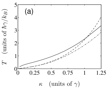
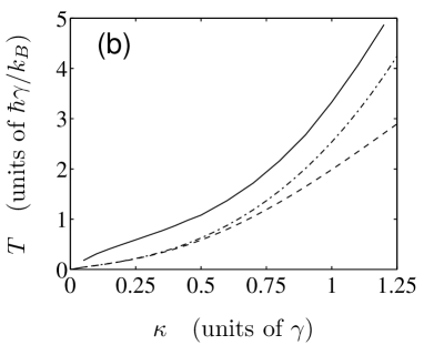
FIG. 1.: Steady-state temperature versus cavity decay rate for (a) $\Delta_{A}=20\gamma$, $\Delta_{C}=0$ and (b) $\Delta_{A}=-20\gamma$, $\Delta_{C}=U_{0}=0.312\gamma$. Solid curves show the numerical results obtained from our semiclassical model. The other curves correspond to the analytical results in the weak-driving limit without (dashed) and with (dash-dotted) adiabatic elimination of the atomic excited state. The other parameters are $\eta=3\kappa$, $g=2.5\gamma$, $\gamma=2\pi\times 3$MHz (rubidium atoms).

In order to study the effects of localisation in more detail, we show in Fig. 2(a) the dependence of the steady-state temperature on the pump strength when all other parameters are kept constant. We see that for decreasing pump strength (decreasing photon number) the temperature approaches the analytic result of the weak-excitation limit. Note that for very small photon numbers of 1 or 2 our semiclassical model is no longer valid and the numerical results exhibit a residual deviation from the analytical ones. (One of the numerical signatures of the limited validity of our model in this parameter regime is the occurence of a negative eigenvalue of the diffusion matrix $\bf D$, Eq. (19), in single particle trajectories.)

Figure 2(a) also shows the ratio of the steady-state temperature and the time-averaged optical potantial depth given by the optical potential times the average photon number $U_{0}\langle n\rangle$, with $n=a^{\dagger}a$. In the weak driving limit, this ratio is much larger than one, indicating a nearly flat atomic distribution in position space. For stronger pumping, the ratio is continuously decreasing and drops well below unity corresponding to strong localisation. This indicates a strong local cooling force, that is, even a particle which is trapped within a single potential well experiences a friction force. Hence, in order to achieve good trapping of particles in the cavity QED domain, one should go to higher photon numbers than those which are currently used in experiments, despite the corresponding higher steady-state temperatures. We will return to the discussion of trapping times in the following section.

Finally, we show in Fig. 2(b) the averaged spatial distribution of a particle for two different values of the pump strength. This again shows the stronger localisation for increasing $\eta$. Moreover, the dashed lines give the spatial distribution of a particle obtained from a thermal distribution with the same mean temperature and a sinusoidal potential of the same mean depth, that is,

$$P_{\mbox{therm}}(x)\propto\exp\left(-\frac{U_{0}\langle n\rangle\cos^{2}(kx)}{k_{B}T}\right).$$ (23)

Note that the numerically obtained distribution strongly deviates from a thermal one due to dynamical effects and the corresponding correlations between atomic degrees of freedom and the cavity field.

 

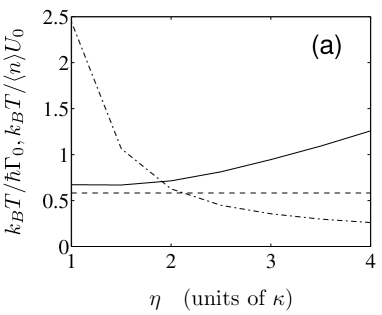
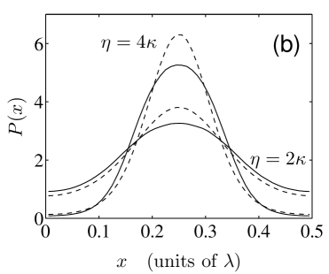
FIG. 2.: Effects of localisation for different pump strengths. (a) Steady-state temperature $T$ versus $\eta$ (solid line), temperature obtained from the analytic solution in the weak-driving limit (dashed), and ratio of $T$ and the mean optical potential $U_{0}\langle n\rangle$. (b) Atomic position distributions within a potential well for $\eta=2\kappa$ and $\eta=4\kappa$ (solid lines), respectively, as compared with thermal distributions (dashed) of the same temperature and the same mean potential. For this plots $\kappa=\gamma/2$ and the other parameters are as in Fig. 1(a).

IV Trapping times

For cavity QED experiments, especially in view of potential applications in quantum information processing, it is an important issue how long the particles can be trapped in the potential wells. Depending on the initial condition, there are different ways to discuss the trapping time of an atom in a well.

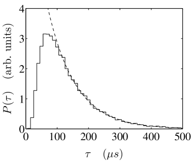
FIG. 3.: Probability distribution $P(\tau)$ for the times at which an atom initially in the ground state of a potential well leaves this well. The solid line is a histogram obtained numerically and the dashed line is an exponential fit. The parameters are those of Fig. 2(b) and $\eta=2\kappa$.

At time $t=0$ the atom can be assumed in the ground state of the potential well. The potential is approximately harmonic so the Wigner function of the ground state of a harmonic oscillator can be used as initial distribution in the semiclassical Monte-Carlo simulations. For a large statistical ensemble we then record the times $\tau$ when the atoms leave the initial potential well. A typical example for the resulting distribution $P(\tau)$ is presented in figure 3. We find a low probability that an atom leaves the potential well at short times since it takes a while until the particle is sufficiently heated by momentum diffusion. For larger times the distribution becomes exponentially decaying $P(\tau)\approx\exp(-\tau/T_{\mbox{trap}})$, e.g., for the given parameters and $\tau>100\mu s$ a fit yields the trapping time $T_{\mbox{trap}}=88.3\mu s$. Note that this initial state is in fact realised in recent experiments [4] where atoms from a magneto-optical trap are velocity selected through the narrow cavity entrance slits before they interact with the optical field, and thus the atoms are effectively prepared in their motional ground state as an initial condition.

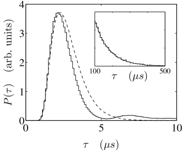
FIG. 4.: Distribution of flight times which an atom spends within single potential wells when it is observed for a very long time. The solid line shows the numerical results, the dashed line is the result for a thermal ensemble of atoms in a static potential for comparison. The inset shows an exponential fit (dashed curve) for long times $\tau$. The parameters are the same as in Fig. 3.

Alternatively one could consider a thermalised atom as initial condition. In this case we simulate a single atom trajectory for a very long period and record the times $\tau$ which the atom spends within a potential well. In the following we will call $\tau$ a “flight time” in order to distinguish it from the trapping time $T_{\mbox{trap}}$ as defined before. We then obtain a distribution for short and long flight times as presented in Figure 4.

As a help for the interpretation of this curve, let us first discuss the corresponding distribution obtained for a thermal ensemble with the same temperature and in a static (conservative) potential of the same depth $\langle n\rangle U_{0}$. In this case there is no momentum diffusion and hence an atom which is trapped initially will stay within the same potential well for arbitrarily long times. Therefore only hot atoms with a total energy larger than the optical potential depth will contribute to the distribution function of flight times which is shown by the dashed curve in Fig. 4. This distribution function shows no flight times $\tau<1\mu s$ that would correspond to very fast atoms, a single maximum at $\tau\approx 2.3\mu s$, and a continuously decreasing probability for longer flight times.

Taking the full cavity dynamics into account has two main effects. First, because of momentum diffusion every atom undergoes a random walk in momentum space and thus will leave a given potential well after a finite time. Second, if an atom enters a potential well with a not too high velocity, it will be slowed down due to the cavity-mediated friction force and thus can be trapped for a longer time. This effect manifests itself in the decrease of the distribution function for times $2\mu s<\tau<6\mu s$ compared to the conservative motion limit. However, in general a particle which just has been trapped will have an energy only slightly below the potential maximum and therefore a relatively high probability of being ejected from the well within a short time. This leads to the second maximum of the distribution function at $\tau\approx 7\mu s$.

Finally, for long times the exponential distribution of the trapping times is detected again, with $T_{\mbox{trap}}=80.5\mu s$, in reasonable agreement with the previous result in Fig. 3. Note, however, that the two definitions for the trapping time $T_{\mbox{trap}}$ are qualitatively different: in Fig. 3 the distribution is obtained from an ensemble of statistically independent atoms, whereas in Fig. 4 only a single atom is followed. Hence in the latter case the distribution exhibits a certain memory of the particle history. For example, a very fast atom will travel over many potential wells and thus will produce many entries in the distribution at short flight times until it gets slowed down and trapped. Because of this the large maximum at times $1\mu s<\tau<5\mu s$ in Fig. 4 only corresponds to about 22% of the total time for which the atom was observed. This also agrees well with the fraction of 20.4% of atoms with energies above the potential barrier obtained from a thermal ensemble, which further supports our interpretation of the distribution function $P(\tau)$ in terms of trapped and untrapped atoms.

The above outlined method for calculating the characteristic trapping time $T_{\mbox{trap}}$ has been carried out for different parameter settings. The trapping time as a function of $\kappa$ and of the pump strength $\eta$ is shown in Figures 5 and 6, respectively.

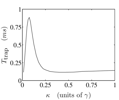
FIG. 5.: Trapping time $T_{\mbox{trap}}$ versus $\kappa$. The parameters for this plot are those of Fig. 1(a).

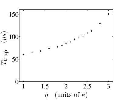
FIG. 6.: Trapping time $T_{\mbox{trap}}$ versus pump strength $\eta$ with $\kappa=\gamma/2$. The parameters are the same as in Fig. 2.

Figure 5 is similar to the analysis of Fig. 1(a), where the photon number is kept approximately constant by a fixed ratio of $\eta/\kappa=3$, and the cavity-induced effects are modified by varying the cavity decay rate $\kappa$. Depending on the value of $\kappa$ we find three very distinct regimes for the behaviour of the trapping time. First, there is a strong increase of the trapping time for very small decay rates. This is due to the strong coupling of the photon number to the atomic position in this limit: already a small elongation of an atom from the field node is sufficient to shift the cavity out of resonance and to drastically reduce the photon number. Thus, the atom dynamically reduces the trapping potential and subsequently can easily leave the potential well. Hence the trapping times are short in this limit. For $\kappa>U_{0}$ the photon number can at most be changed by a factor of two by the atom and the behaviour of the trapping time is no longer dominated by this dynamical effect. In this regime the photon number and consequently the potential depth are approximately constant, but the temperature of the atom increases with increasing $\kappa$ as we have seen in Fig. 1(a). Thus the atomic localisation decreases, which in turn gives rise to a decrease of the trapping time. Finally, we find again a slight increase of the trapping time when $\kappa$ is so large that the temperature is of the order of or larger than the optical potential depth. An increase of $\kappa$ then still increases the temperature and thus the fraction of untrapped particles. However, our definition of the trapping time as the exponential decay of the flight time distribution for very long times (Fig. 4) relies on the trapped particles only and does not depend on the fraction of untrapped atoms. The trapping time is then dominated by the time scale of the friction force and of the momentum diffusion, which becomes longer for large increasing $\kappa$. This is due to approaching the classical potential limit for $\kappa\rightarrow\infty$ with a fixed ratio $\eta/\kappa$. This explains the final increase of the trapping time in Fig. 5.

In Figure 6 the photon number is varied by $\eta$, while the other parameters are kept constant. Though the temperature gets higher with increasing photon numbers (see Fig. 2), the resulting trapping times exhibit a considerable increase owing to the strong deepening of the potential wells. This result suggests clearly the benefit of working in an intermediate photon number regime for implementing coherent manipulation with neutral atoms in optical lattices.

V Conclusions

We have derived semiclassical stochastic differential equations to simulate the coupled dynamics of an atom moving in a single cavity mode in the limit of strong nonresonant interaction between the field and the atomic dipole. Starting from the basic quantum equations we performed systematic approximations such that the model accounts consistently for the quantum noise properties of the system. A nontrivial correlation between the field phase noise and the momentum noise has been revealed and can be interpreted in terms of simple physical processes.

As an example for our method we have studied the atomic motion in a one dimensional optical lattice sustained by the strongly coupled cavity field. In the appropriate limits the calculated steady-state temperatures are in good agreement with the results of previous calculations. Deviations can be attributed to atomic localisation within the potential wells, which is consistently described in our semiclassical simulation. We found that for higher intracavity photon numbers the characteristic trapping times can be significantly increased up to milliseconds. In this case the potential wells get deeper and diffusion and friction are enhanced in a way that the temperature only slowly increases. Hence the steady state temperature can get significantly smaller than the well depth. Alternatively by simultaneously increasing the atom-field detuning, we can keep the effective potential the same but reduce diffusion to achieve longer storage times. As the calculational effort only weakly depends on the photon number we can nicely study the transition from a quantum to a classical field.

Let us mention here that the model can easily be generalised to 3D, more cavity modes and several atoms simultaneously in the cavity. Hence, this semiclassical approach offers a tool for a tractable numerical simulation of the dynamics of these complex systems. These simulations could then be used to check the performance of atom cavity systems for quantum computing and quantum information processing.

REFERENCES

- [1] see e.g. Cavity Quantum Electrodynamics, edited by P. R. Berman (Academic Press, San Diego, 1994).
- [2] P. Horak, G. Hechenblaikner, K. M. Gheri, H. Stecher, and H. Ritsch, Phys. Rev. Lett. 79, 4974 (1997).
- [3] C. J. Hood, T. W. Lynn, A. C. Doherty, A. S. Parkins, and H. J. Kimble, Science 287, 1447 (2000).
- [4] P. W. H. Pinkse, T. Fischer, P. Maunz, and G. Rempe, Nature 404, 365 (2000).
- [5] G. Hechenblaikner, M. Gangl, P. Horak, and H. Ritsch, Phys. Rev. A 58, 3030 (1998).
- [6] P. Münstermann, T. Fischer, P. Maunz, P. W. H. Pinkse, and G. Rempe, Phys. Rev. Lett. 84, 4068 (2000).
- [7] M. Gangl and H. Ritsch, Phys. Rev. A 61, 043405 (2000).
- [8] A. Hemmerich, Phys. Rev. A 60, 943 (1999).
- [9] P. Zoller, Nature 404, 340 (2000).
- [10] C. Cohen-Tannoudji, in “Fundamental Systems in Quantum Optics”, Proceedings of the Les Houches Summer School 1990, Session LIII, edited by J. Dalibard, J.-M. Raimond, and J. Zinn-Justin (Elsevier Science, Amsterdam, 1992).
- [11] J. Dalibard and C. Cohen-Tannoudji, J. Phys. B. 18, 1661 (1985).
- [12] A. C. Doherty, A. S. Parkins, S. M. Tan, and D. F. Walls, Phys. Rev. A 56, 833 (1997).
- [13] A. C. Doherty, T. W. Lynn, C. J. Hood, and H. J. Kimble, quant-ph/0006015.
- [14] C. W. Gardiner and P. Zoller, Quantum Noise, 2nd edition (Springer-Verlag, Berlin, 2000).
- [15] J. Javanainen, Phys. Rev. A 46, 5819 (1992).
- [16] Y. Castin, K. Berg-Sørensen, J. Dalibard, and K. Mølmer, Phys. Rev. A 50, 5092 (1994).
- [17] K. I. Petsas, G. Grynberg, and J.-Y. Courtois, Eur. Phys. J. D 6, 29 (1999).
- [18] C. W. Gardiner, Handbook of Stochastic Methods (Springer-Verlag, Berlin, 1985).
- [19] V. Vuletic and S. Chu, Phys. Rev. Lett. 84, 3787 (1999).