The effects of time delays in adaptive phase measurements

Abstract

It is not possible to make measurements of the phase of an optical mode using linear optics without introducing an extra phase uncertainty. This extra phase variance is quite large for heterodyne measurements, however it is possible to reduce it to the theoretical limit of $\log\bar{n}/(4\bar{n}^{2})$ using adaptive measurements. These measurements are quite sensitive to experimental inaccuracies, especially time delays and inefficient detectors. Here it is shown that the minimum introduced phase variance when there is a time delay of $\tau$ is $\tau/(8\bar{n})$. This result is verified numerically, showing that the phase variance introduced approaches this limit for most of the adaptive schemes using the best final phase estimate. The main exception is the adaptive mark II scheme with simplified feedback, which is extremely sensitive to time delays. The extra phase variance due to time delays is considered for the mark I case with simplified feedback, verifying the $\tau/2$ result obtained by Wiseman and Killip both by a more rigorous analytic technique and numerically.

1 Introduction

It is well known that any measurement of the phase of an electromagnetic field using linear optics will have an uncertainty that is greater than the intrinsic quantum phase uncertainty of the state fullquan . The standard phase measurement method is the heterodyne scheme, where the signal is combined with a strong local oscillator field with a slightly different frequency. This means that all quadratures of the field are sampled approximately equally. This phase measurement method introduces a phase variance of approximately $1/(4\bar{n})$, where $\bar{n}$ is the mean photon number of the field.

This is not so significant for measurements on coherent states, where it is the same size as the intrinsic phase uncertainty of the state. For states with reduced phase uncertainty, however, the uncertainty in the measurement will be far greater than the intrinsic phase uncertainty. For example, minimum phase uncertainty states have a phase variance that scales as $1/(\bar{n}^{2})$ SumPeg90 .

It is possible to dramatically improve on heterodyne measurements by using a local oscillator phase of $\Phi=\varphi+\pi/2$, where $\varphi$ is the signal phase (homodyne detection). This has the drawback that the phase must be known in advance. Adaptive phase measurements fullquan ; Wis95c ; semiclass ; BerWisZha99 ; unpub attempt to approximate a homodyne phase measurement by adjusting the local oscillator phase based on data obtained during the measurement.

There are several different variations of adaptive phase measurements. The adaptive mark I scheme gives improved results for small photon numbers, but worse results for large photon numbers. The adaptive mark II scheme gives an introduced phase variance of $1/(8\bar{n}^{1.5})$ semiclass ; BerWisZha99 , a significant improvement over heterodyne measurements. By a more sophisticated feedback algorithm it is even possible to obtain the theoretical limit of $\log{\bar{n}}/(4\bar{n}^{2})$ unpub .

These adaptive measurement schemes are sensitive to experimental imperfections, most notably imperfect detectors and time delays. The effect of imperfect detectors is fairly straightforward, introducing a phase variance of approximately $(1-\eta)/(4\eta\bar{n})$ semiclass . The effect of time delays is more difficult to estimate. Some highly simplified calculations indicate that the excess phase variance due to time delays is $\tau/2$ for mark I measurements (where $\tau$ is the time delay), and $\tau/(2\bar{n})$ for mark II measurements semiclass .

Here we repeat these derivations more accurately, and show that while the result for mark I measurements is reasonably accurate, the perturbation approach is inadequate to obtain a consistent result for mark II measurements. We consider an alternative derivation that gives the minimum phase variance when there is a time delay. In section 5 we evaluate the phase variance with time delays numerically and show that for most of the measurement schemes the phase variance approaches this limit for large time delays.

2 Background theory

Before we proceed to determining the effect of time delays, we will briefly outline the background theory for adaptive measurements. For more details see fullquan ; semiclass . First the photocurrent for dyne detection fullquan is given by

$$I(v){\rm d}v=2{\rm Re}(\alpha_{v}e^{-i\Phi(v)}){\rm d}v+{\rm d}W(v).$$ (1)

Here $\alpha_{v}$ is the scaled coherent amplitude of the signal, $v$ is the scaled time and $\Phi(v)$ is the local oscillator phase. The systematic variation with time of the coherent amplitude due to the mode shape is scaled out, and time is scaled to the unit interval. We also define the variables

$$A_{v} =\int_{0}^{v}I(u)e^{i\Phi(u)}{\rm d}u,$$ (2)

$$B_{v} =-\int_{0}^{v}e^{2i\Phi(u)}{\rm d}u,$$ (3)

$$C_{v} =A_{v}v+B_{v}A_{v}^{*}.$$ (4)

We omit the subscripts to indicate final values. The best estimate of the phase at time $v$ is given by $\arg C_{v}$, and if $|B_{v}|$ is small then $\arg A_{v}$ is also a good phase estimate.

For mark I measurements $\arg A_{v}$ is used as the intermediate phase estimate (so the local oscillator phase is $\Phi=\arg A_{v}+\pi/2$) and also as the phase estimate at the end of the measurement. For mark II measurements we use the same intermediate phase estimate but we use the best estimate $\arg C$ at the end of the measurement. In semiclass it is shown that using $\arg A_{v}$ as the intermediate phase estimate is equivalent to varying the local oscillator phase as

$${\rm d}\Phi(v)=\frac{I(v){\rm d}v}{\sqrt{v}}.$$ (5)

Using the feedback in this form allows us to use a simplified feedback circuit experimentally. This feedback is no longer equivalent to using a phase estimate of $\arg A_{v}$ when there are time delays in the system, and we therefore consider the cases with $\arg A_{v}$ feedback and simplified feedback separately.

The next feedback scheme uses a phase estimate intermediate between $\arg A_{v}$ and $\arg C_{v}$, specifically

$$\hat{\varphi}=\arg(A_{v}^{\epsilon}C_{v}^{1-\epsilon}).$$ (6)

The simplest case is where $\epsilon$ does not depend on time. For each mean photon number there is an optimum value to use, and provided these optimum values are used this method gives better results than mark II measurements unpub .

We can get very close to the theoretical limit of $\log\bar{n}/(4\bar{n}^{2})$ if we use a time dependent $\epsilon$ given by unpub

$$\epsilon(v)=\frac{v^{2}-|B_{v}|^{2}}{|C_{v}|}\sqrt{\frac{v}{1-v}}.$$ (7)

Briefly explaining the reason for the theoretical limit, the probability distribution for $A$ and $B$ is proportional to $|\langle{\beta,\zeta}|{\psi}\rangle|^{2}$, where $|{\psi}\rangle$ is the signal state and $|{\beta,\zeta}\rangle$ is a squeezed state

$$|{\beta,\zeta}\rangle=\exp(\beta a^{\dagger}-{{\beta}}^{*}a)\exp[\tfrac{1}{2}\zeta^{*}a^{2}-\tfrac{1}{2}\zeta(a^{\dagger})^{2}]|{0}\rangle,$$ (8)

where

$$\beta =\frac{C}{1-B^{2}},$$ (9)

$$\zeta =-\frac{B{\rm atanh}|B|}{|B|}.$$ (10)

This means that the phase variance introduced is approximately equal to the phase variance of the squeezed state $|{\beta,\zeta}\rangle$. The photon number of this squeezed state will be approximately the same as that of the input state, so the theoretical minimum introduced phase variance is that of an optimized squeezed state with photon number $\bar{n}$. As shown in collett , this scales as $\log{\bar{n}}/\bar{n}^{2}$.

The phase measurement scheme with time dependent $\epsilon$ (7) is not quite at the theoretical limit because it produces squeezed states $|{\beta,\zeta}\rangle$ that are slightly more highly squeezed than optimum. In unpub we show how this can be corrected, but we will not consider the case with these corrections here because the time delays cause the squeezed state to be less squeezed than optimum anyway, so these corrections are not needed.

3 Perturbation approach

3.1 Mark I

Now we estimate the effect of time delays on simplified mark I measurements in a similar way to that done in semiclass , but using fewer of the simplifications used there. Without a time delay the stochastic differential equation (SDE) for the phase estimate is

$${\rm d}\hat{\varphi}_{v} =\frac{I(v){\rm d}v}{\sqrt{v}}$$

$$=v^{-1/2}[-2\alpha\sin\hat{\varphi}_{v}{\rm d}v+{\rm d}W(v)].$$ (11)

In this expression we have taken the input phase to be zero. For some time $v_{1}$ the phase will come to lie near 0, so we linearise around $\hat{\varphi}_{v}=0$. The result, which will be valid for $v_{1}\leq v\leq 1$ is

$${\rm d}\hat{\varphi}_{v}=v^{-1/2}[-2\alpha\hat{\varphi}_{v}{\rm d}v+{\rm d}W(v)].$$ (12)

Including the time delay the SDE is

$${\rm d}\hat{\varphi}_{v}=v^{-1/2}[-2\alpha\hat{\varphi}_{v-\tau}{\rm d}v+{\rm d}W(v)].$$ (13)

Now we treat the delay perturbatively. We write the solution to the perturbed equation as

$$\hat{\varphi}_{v}=\hat{\varphi}_{v}^{(0)}+\alpha\tau\hat{\varphi}_{v}^{(1)}+O(\alpha^{2}\tau^{2}).$$ (14)

The zeroth-order term obeys the SDE for no delay (12), so the first-order correction obeys

$$\alpha\tau{\rm d}\hat{\varphi}_{v}^{(1)}=2\alpha v^{-1/2}(\hat{\varphi}_{v}^{(0)}-\hat{\varphi}_{v-\tau}^{(0)}){\rm d}v-2\alpha^{2}\tau v^{-1/2}\hat{\varphi}_{v-\tau}^{(1)}{\rm d}v.$$ (15)

Therefore to first order in $\tau$ we have

$${\rm d}\hat{\varphi}_{v}^{(1)} =2v^{-1/2}{\rm d}\hat{\varphi}_{v}^{(0)}-2\alpha v^{-1/2}\hat{\varphi}_{v}^{(1)}{\rm d}v$$

$$=2v^{-1/2}\{v^{-1/2}[-2\alpha\hat{\varphi}_{v}^{(0)}{\rm d}v+{\rm d}W(v)]\}-2\alpha v^{-1/2}\hat{\varphi}_{v}^{(1)}{\rm d}v$$

$$=-2\alpha v^{-1/2}\hat{\varphi}_{v}^{(1)}{\rm d}v-\frac{4\alpha}{v}\hat{\varphi}_{v}^{(0)}{\rm d}v+\frac{2}{v}{\rm d}W(v).$$ (16)

It is straightforward to show that the solution to the zeroth-order equation is

$$\hat{\varphi}_{v}^{(0)}=e^{4\alpha(\sqrt{v_{1}}-\sqrt{v})}\hat{\varphi}_{v_{1}}^{(0)}+\int_{v_{1}}^{v}\frac{e^{4\alpha(\sqrt{u}-\sqrt{v})}}{\sqrt{u}}{\rm d}W(u).$$ (17)

Using this in equation (16) and multiplying on both sides by $e^{4\alpha\sqrt{v}}$ gives

$${\rm d}(e^{4\alpha\sqrt{v}}\hat{\varphi}_{v}^{(1)})=-\frac{4\alpha}{v}\left[e^{4\alpha\sqrt{v_{1}}}\hat{\varphi}_{v_{1}}^{(0)}+\int_{v_{1}}^{v}\frac{e^{4\alpha\sqrt{u}}}{\sqrt{u}}{\rm d}W(u)\right]{\rm d}v+\frac{2}{v}e^{4\alpha\sqrt{v}}{\rm d}W(v).$$ (18)

Integrating then gives the solution

$$\hat{\varphi}_{v}^{(1)} =e^{4\alpha(\sqrt{v_{1}}-\sqrt{v})}\hat{\varphi}_{v_{1}}^{(1)}-\int_{v_{1}}^{v}\frac{4\alpha}{s}\left[e^{4\alpha(\sqrt{v_{1}}-\sqrt{v})}\hat{\varphi}_{v_{1}}^{(0)}\vphantom{\frac{e^{4\alpha(\sqrt{u}-\sqrt{v})}}{\sqrt{u}}}\right.$$

$$\left.+\int_{v_{1}}^{s}\frac{e^{4\alpha(\sqrt{u}-\sqrt{v})}}{\sqrt{u}}{\rm d}W(u)\right]{\rm d}s+\int_{v_{1}}^{v}\frac{2}{s}e^{4\alpha(\sqrt{s}-\sqrt{v})}{\rm d}W(s).$$ (19)

In this approximation the mark I phase estimate is given by $\hat{\varphi}_{1}=\hat{\varphi}_{1}^{(0)}+\alpha\tau\hat{\varphi}_{1}^{(1)}$. To first order in $\tau$ and $\alpha^{-1}$ this has a variance of

$$\left\langle{\phi_{\rm I}^{2}}\right\rangle=\frac{1}{4\alpha}+2\alpha\tau\left\langle{\hat{\varphi}_{1}^{(0)}\hat{\varphi}_{1}^{(1)}}\right\rangle.$$ (20)

Here we have used the known variance of $1/(4\alpha)$ of the zeroth-order term. Evaluating the second term on the right-hand side we find

$$\left\langle{\hat{\varphi}_{1}^{(0)}\hat{\varphi}_{1}^{(1)}}\right\rangle =e^{-8\alpha(1-\sqrt{v_{1}})}\left\langle{\hat{\varphi}_{v_{1}}^{(0)}\hat{\varphi}_{v_{1}}^{(1)}}\right\rangle+4\alpha\log(v_{1})e^{-8\alpha(1-\sqrt{v_{1}})}\left\langle{{\hat{\varphi}_{v_{1}}^{(0)2}}}\right\rangle$$

$$-\int_{v_{1}}^{1}\frac{4\alpha}{s}\int_{v_{1}}^{s}\frac{e^{8\alpha(\sqrt{u}-1)}}{u}{\rm d}u{\rm d}s+\int_{v_{1}}^{1}\frac{2e^{8\alpha(\sqrt{u}-1)}}{u^{1.5}}{\rm d}u.$$ (21)

The first two terms decrease exponentially with $\alpha$ and may therefore be omitted. Exchanging the order of the integrals in the third term and integrating gives

$$\left\langle{\hat{\varphi}_{1}^{(0)}\hat{\varphi}_{1}^{(1)}}\right\rangle=4\alpha\int_{v_{1}}^{1}\frac{\log u}{u}e^{8\alpha(\sqrt{u}-1)}{\rm d}u+\int_{v_{1}}^{1}\frac{2e^{8\alpha(\sqrt{u}-1)}}{u^{1.5}}{\rm d}u.$$ (22)

Now we change variables to $s=1-\sqrt{u}$, so ${\rm d}u=-2(1-s){\rm d}s$. Then we obtain

$$\left\langle{\hat{\varphi}_{1}^{(0)}\hat{\varphi}_{1}^{(1)}}\right\rangle=16\alpha\int_{0}^{1-\sqrt{v_{1}}}\frac{\log(1-s)}{(1-s)}e^{-8\alpha s}{\rm d}s+4\int_{0}^{1-\sqrt{v_{1}}}\frac{e^{-8\alpha s}}{(1-s)^{2}}{\rm d}s.$$ (23)

Expanding in a Maclaurin series in $s$ gives

$$\left\langle{\hat{\varphi}_{1}^{(0)}\hat{\varphi}_{1}^{(1)}}\right\rangle =-16\alpha\int_{0}^{1-\sqrt{v_{1}}}(s+\frac{3}{2}s^{2}+O(s^{3}))e^{-8\alpha s}{\rm d}s$$

$$+4\int_{0}^{1-\sqrt{v_{1}}}(1+2s+3s^{2}+O(s^{3})){e^{-8\alpha s}}{\rm d}s$$

$$=-16\alpha\left[\frac{1}{(8\alpha)^{2}}+\frac{3}{(8\alpha)^{3}}+O(\alpha^{-4})\right]$$

$$+4\left[\frac{1}{8\alpha}+\frac{2}{(8\alpha)^{2}}+\frac{6}{(8\alpha)^{3}}+O(\alpha^{-4})\right]$$

$$=\frac{1}{4\alpha}+O(\alpha^{-2}).$$ (24)

Note that the upper bound at $1-\sqrt{v_{1}}$ has no effect since it gives a term that decays exponentially with $\alpha$. Thus we find that the total phase variance is

$$\left\langle{\phi_{\rm I}^{2}}\right\rangle=\frac{1}{4\alpha}+\frac{\tau}{2}.$$ (25)

This provides a good verification of the result obtained by the highly simplified method in semiclass .

Note that this result is based on continuing to use the intermediate phase estimate at the end of the measurement. If we use the phase estimate $\arg A$ at the end of the measurement we will get a different result, one that we cannot predict using this approach.

3.2 Mark II

If we try to use the same approach for the mark II case it does not seem to be possible to obtain a consistent result. To illustrate this, we will briefly outline the derivation. From semiclass , the mark II phase estimate is effectively a time average of the mark I phase estimates:

$$\phi_{\rm II}\approx\int_{0}^{1}\hat{\varphi}_{t}{\rm d}t.$$ (26)

In order for this to be consistent with the above theory we will take the average only from time $v_{1}$, then take the limit of small $v_{1}$. In perturbation theory the mark II phase estimate is

$$\phi_{\rm II}=\int_{v_{1}}^{1}[\hat{\varphi}_{t}^{(0)}+\alpha\tau\hat{\varphi}_{t}^{(1)}]{\rm d}t.$$ (27)

We find that the variance is

$$\left\langle{\phi_{\rm II}^{2}}\right\rangle=\int_{v_{1}}^{1}{\rm d}t\int_{v_{1}}^{1}{\rm d}t^{\prime}\left\langle{\hat{\varphi}_{t}^{(0)}\hat{\varphi}_{t^{\prime}}^{(0)}}\right\rangle+2\alpha\tau\int_{v_{1}}^{1}{\rm d}t\int_{v_{1}}^{1}{\rm d}t^{\prime}\left\langle{\hat{\varphi}_{t}^{(0)}\hat{\varphi}_{t^{\prime}}^{(1)}}\right\rangle.$$ (28)

The first term is fairly well behaved, and in the limit of small $v_{1}$ we get

$$\int_{v_{1}}^{1}{\rm d}t\int_{v_{1}}^{1}{\rm d}t^{\prime}\left\langle{\hat{\varphi}_{t}^{(0)}\hat{\varphi}_{t^{\prime}}^{(0)}}\right\rangle\approx\frac{1}{4\alpha^{2}}.$$ (29)

Expanding the second term in equation (28) gives

$$\int_{v_{1}}^{1}{\rm d}t\int_{v_{1}}^{1}{\rm d}t^{\prime}\left\langle{\hat{\varphi}_{t}^{(0)}\hat{\varphi}_{t^{\prime}}^{(1)}}\right\rangle= \int_{v_{1}}^{1}{\rm d}t\int_{v_{1}}^{1}{\rm d}t^{\prime}\left[e^{4\alpha(2\sqrt{v_{1}}-\sqrt{t}-\sqrt{t^{\prime}})}\left\langle{\hat{\varphi}_{v_{1}}^{(0)}\hat{\varphi}_{v_{1}}^{(1)}}\right\rangle\vphantom{\int_{v_{1}}^{t^{\prime}}}\right.$$

$$\left.-\int_{v_{1}}^{t^{\prime}}\frac{4\alpha}{s}e^{4\alpha(2\sqrt{v_{1}}-\sqrt{t}-\sqrt{t^{\prime}})}\left\langle{{\hat{\varphi}_{v_{1}}^{(0)2}}}\right\rangle{\rm d}s\right.$$

$$\left.-\int_{v_{1}}^{t^{\prime}}\frac{4\alpha}{s}{\rm d}s\int_{v_{1}}^{t}\int_{v_{1}}^{s}\frac{e^{4\alpha(\sqrt{v}-\sqrt{t})}}{\sqrt{v}}{\rm d}W(v)\frac{e^{4\alpha(\sqrt{u}-\sqrt{t^{\prime}})}}{\sqrt{u}}{\rm d}W(u)\right.$$

$$\left.+\int_{v_{1}}^{t}\int_{v_{1}}^{t^{\prime}}\frac{e^{4\alpha(\sqrt{v}-\sqrt{t})}}{\sqrt{v}}{\rm d}W(v)\frac{2}{u}e^{4\alpha(\sqrt{u}-\sqrt{t^{\prime}})}{\rm d}W(u)\right].$$ (30)

Simplifying this, the third and fourth terms cancel, and the first two terms give

$$\frac{v_{1}}{4\alpha^{2}}\left\langle{\hat{\varphi}_{v_{1}}^{(0)}\hat{\varphi}_{v_{1}}^{(1)}}\right\rangle-\frac{\sqrt{v_{1}}}{2\alpha^{2}}\left\langle{{\hat{\varphi}_{v_{1}}^{(0)2}}}\right\rangle+O(\alpha^{-3})$$ (31)

Unlike the results for the mark I case, all the terms depend on the conditions at time $v_{1}$. This means that it is not possible to obtain an unambiguous result in the limit $v_{1}\to 0$. Therefore we consider an alternative approach for estimating the increase in the phase variance due to the time delay.

4 Theoretical minimum

The alternative method of obtaining an estimate of the time delay is to consider the squeezed state $|{\beta,\zeta}\rangle$ in the probability distribution. As was explained above, the excess phase variance due to the measurement scheme is approximately the phase variance of this squeezed state.

From collett , the phase variance of a squeezed state is given by

$$\left\langle{\Delta\phi^{2}}\right\rangle\approx\frac{n_{0}+1}{4\bar{n}_{\rm p}^{2}}+2{\rm erfc}\left(\sqrt{2n_{0}}\right),$$ (32)

where $n_{0}=\bar{n}_{\rm p}e^{2\zeta}$ for real $\zeta$. Here we use the subscript p to indicate the mean photon number of the squeezed state in the probability distribution, as opposed to the photon number of the input state. The average value of $\bar{n}_{\rm p}$ will be close to the photon number of the input state.

For states that are significantly less squeezed than optimum, the second term is negligible and we can omit the term of order $\bar{n}_{\rm p}^{-2}$. Then this simplifies to

$$\left\langle{\Delta\phi^{2}}\right\rangle\approx\frac{e^{2\zeta}}{4\bar{n}_{\rm p}}.$$ (33)

Since $\bar{n}_{\rm p}$ will be close to the photon number of the input state, it is reasonable to replace it with $\bar{n}$.

When we have a delay of $\tau$ in the system, before time $\tau$ we have no information about the phase of the system to use to adjust the local oscillator phase. Therefore we must use a heterodyne scheme for this time period, rapidly varying the local oscillator phase. This means that $B_{\tau}$ will be equal to zero, and no matter how good the phase estimate is after time $\tau$, the largest the magnitude of $B_{v}$ can be made is $v-\tau$. Then at the end of the measurement, the largest $|B|$ can be is $1-\tau$, and the largest $|\zeta|$ can be is ${\rm atanh}(1-\tau)$.

The lower limit to the phase variance of $|{\beta,\zeta}\rangle$ when there is a time delay of $\tau$ is therefore

$$\left\langle{\Delta\phi^{2}}\right\rangle_{{\rm min}} \approx\frac{e^{-2{\rm atanh}(1-\tau)}}{4\bar{n}},$$ (34)

$$\approx\frac{\tau}{8\bar{n}}.$$ (35)

This is therefore also the lower limit to the introduced phase variance when there is a time delay of $\tau$. We can expect that the introduced phase variance will be close to this for states of small intrinsic phase variance, as there will quickly be very good phase estimates available for the feedback phase. In addition the time delay must be sufficiently large that the phase variance given by this expression is significantly above the introduced phase variance for no time delay.

This result obeys the same scaling law as the result given in semiclass , but it is a factor of four times smaller. Note, however, that the limit condition for the result given in semiclass is that $\tau\alpha$ is small, whereas the above result should only be accurate when both $\alpha$ and $\tau$ are reasonably large. The result here also differs in that it is the limit for the total introduced phase variance, rather than just the extra phase variance due to the time delay.

5 Numerical results

These analytic results were also tested numerically. The numerical techniques used were similar to those used in reference unpub . Minimum uncertainty squeezed states were used, with the stochastic differential equations for the squeezing parameters rigo as given in unpub . For all calculations $2^{20}$ time steps were used, and calculations were performed with time delays of $2^{n}$ time steps, where $n$ varies from 0 to 18.

For the first $2^{n}$ time steps the local oscillator phase was rotated by $\pi/2$ each step. For the following time steps the data up to the time step $2^{n}$ before the current time step was used. For a delay of $2^{0}=1$ time steps the data from the previous step is used, corresponding to the technique for no time delay.

Numerical results for four different phase feedback schemes were obtained:

(a) The simplified feedback for mark I and II measurements, where

$${\rm d}\hat{\varphi}_{v}=\frac{I(v){\rm d}v}{\sqrt{v}}.$$ (36)

(b) The unsimplified feedback, where the phase estimate is

$$\hat{\varphi}(v)=\arg A_{v}.$$ (37)

(c) The phase estimate that is intermediate between $\arg A_{v}$ and the best phase estimate

$$\hat{\varphi}(v)=\arg\left(A_{v}^{\epsilon}C_{v}^{1-\epsilon}\right),$$ (38)

where $\epsilon$ is a constant.

(d) The same as in (c), except that the value of $\epsilon$ varies with time as

$$\epsilon(v)=\frac{v^{2}-|B_{v}|^{2}}{|C_{v}|}\sqrt{\frac{v}{1-v}}.$$ (39)

5.1 Comparison with perturbative theory

First we consider the case of simplified feedback, and consider the variance in the final value of the feedback phase, rather than the phase of $A$ or $C$. This case was examined in section 3.1, and the extra phase variance due to the time delay is $\tau/2$ according to that analysis. The extra phase variance is plotted for four different mean photon numbers in figure 1.

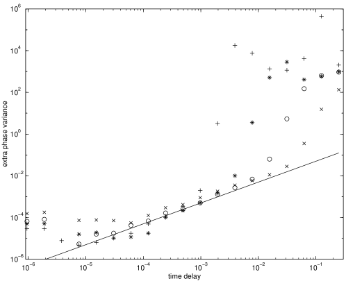
Figure 1: The extra phase variance (in the final value of the intermediate phase estimate for the simplified feedback) due to the time delay plotted as a function of time delay for four different mean photon numbers. The data for a mean photon number of 121.590 is shown as crosses, for a photon number of 1 576.55 as circles, for a photon number of 22 254.8 as asterisks and for a photon number of 332 067 as plusses. The theoretical value of ${\tau}/2$ is plotted as the continuous line.

In determining the extra phase variance due to the time delay, an estimate must be made of the phase variance with no time delay. For the results shown in figure 1, the phase variances are very close for the first six or so time delays. The estimate of the phase variance with no time delay was taken to be the minimum of these results.

The theoretical value of $\tau/2$ is also plotted in figure 1. As can be seen, many of the results are close to the theoretical line for the intermediate time delays. For small time delays the extra phase variance due to the time delay is too small a fraction of the total phase variance for the results to be accurate. The reason why the results deviate from the theoretical result for large time delays is that this theoretical result is for the limit of small $\alpha\tau$. Note also that the results for larger photon numbers deviate from the theoretical result for smaller $\tau$ than the results for smaller photon numbers. This is also to be expected from this limit condition.

We also used fitting techniques to determine how closely the numerical results agree with the theoretical value. A linear fit of the phase variances against $\tau$ was performed, and data for $\alpha\tau$ above about $0.3$ was omitted, as this was where the results started to increase dramatically. The average slope obtained was $0.39\pm 0.06$, in reasonable agreement with the theoretical value of $0.5$.

As was mentioned above, the result for the additional phase variance due to the time delay is only valid for the variance in the final value of the phase estimate, which is not the same as $\arg A$ when there is a time delay. In figure 2 we have plotted the variation of the phase variance with time delay for three alternative final phase estimates, $\hat{\varphi}$, $\arg A$ and $\arg C$. This is for a photon number of approximately 332 000, and is fairly representative of the results for other photon numbers.

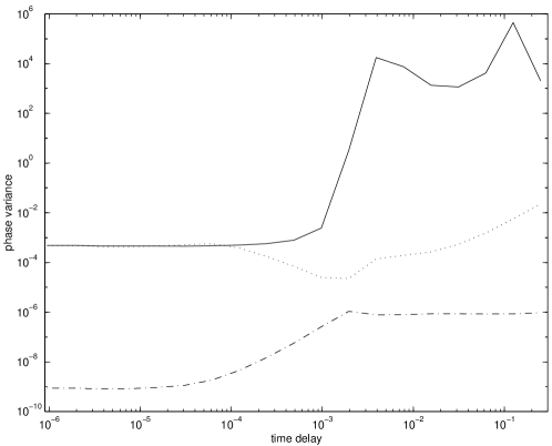
Figure 2: The phase variance of three alternative final phase estimates for simplified feedback with a time delay plotted as a function of time delay. The results for the final value of the intermediate phase estimate are plotted as a continuous line, for $\arg A$ as a dotted line, and for $\arg C$ as a dash-dot line. All results are for a photon number of 332 067.

As can be seen, for very small time delays the variances in the $\hat{\varphi}$ and $\arg A$ phase estimates are almost identical. As the time delay is increased, however, the variance of $\hat{\varphi}$ increases, but the variance of $\arg A$ decreases. This is because, as the intermediate phase estimate gets worse, the value of $|B|$ decreases. This means that $A$ is closer to $C$, so $\arg A$ is closer to the best phase estimate. Note, however, that the variance of $\arg A$ rises again, and does not converge to $\arg C$ for large time delays. This is because $|B|$ does not fall to zero.

5.2 Comparison with theoretical minimum

Now we consider the variance in the phase of $C$. As was explained above, the theoretical lower limit to the introduced phase variance is $\tau/(8\bar{n})$. We have plotted the introduced variance in the best phase estimate $\arg C$ and the theoretical limit in figure 3. For additional accuracy we have plotted

$$\frac{e^{-2{\rm atanh}(1-\tau)}}{4\bar{n}},$$ (40)

as this will continue to be accurate for time delays that are a large fraction of 1. This plot is for a photon number of 332 000, and similar results are obtained for other photon numbers. As can be seen, the phase variance is well above the theoretical limit. For large time delays the phase variance approximately converges to the heterodyne phase variance, also shown in figure 3.

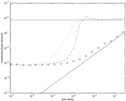
Figure 3: The phase variance introduced for three different phase feedback schemes plotted as a function of time delay. The dotted line is for simplified feedback, the dash-dot line is for the corrected simplified feedback, and the circles are for unsimplified $\arg A_{v}$ feedback. The best phase estimate $\arg C$ is used in all three cases. The continuous horizontal line is the phase variance for heterodyne measurements, and the continuous diagonal line is the theoretical limit. All results are for a photon number of 332 067.

The phase variance introduced for mark II measurements with the unsimplified $\arg A_{v}$ feedback is also shown in figure 3. The phase variance introduced for this case increases far more slowly with the time delay, and for larger time delays it is very close to the theoretical limit. These results indicate that if there is any significant time delay in the system the simplified feedback will give a far worse result than using $\arg A_{v}$.

It is possible to make a correction to the simplified phase feedback scheme that improves this result somewhat. Many different alternatives were tried, and the one that gave the best results was

$${\rm d}\hat{\varphi}_{v}=\frac{I(v){\rm d}v}{\sqrt{v+\alpha\tau}}.$$ (41)

This correction is based on the fact that $|A_{v}|$ is larger than $\sqrt{v}$ when the phase estimate is worse than $\arg A_{v}$. (From semiclass , the factor of $\sqrt{v}$ in the simplified feedback comes from a factor of $|A_{v}|$.)

The results for this correction are also shown in figure 3. The phase variances obtained in this case are significantly below those for the plain simplified feedback, but are still far above the results for the unsimplified $\arg A_{v}$ feedback.

Now we consider the results for better intermediate phase estimates that are between $\arg A_{v}$ and $\arg C_{v}$. The phase variance introduced for the constant $\epsilon$ case and the theoretical limit are shown in figure 4. These results are again for a photon number of about 332 000. The results for this case are even closer to the theoretical limit than those for the mark II case.

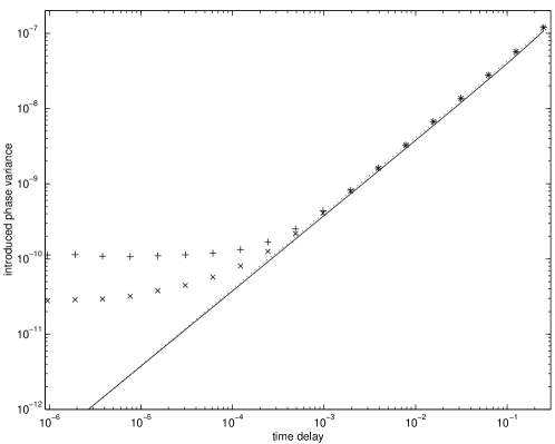
Figure 4: The phase variance introduced for better intermediate phase estimates plotted as a function of time delay. The plusses are for the constant $\epsilon$ case and the crosses are for the time-dependent $\epsilon$ case. The theoretical limit estimated using the mean inverse photon numbers obtained from the time-dependent $\epsilon$ case is plotted as the dotted line, and the theoretical limit using the input photon number is shown as the continuous line. All results are for a photon number of 332 067.

The phase variance introduced for the feedback with time dependent $\epsilon$ is also plotted in figure 4. The results for this case converge to the theoretical limit at smaller time delays than for the constant $\epsilon$ case. For the larger time delays the results for the two cases are about the same, slightly above the theoretical limit.

In both cases we find that for large time delays the phase variance is still noticeably above the theoretical limit, and that the values of $B$ obtained are too close to $1-\tau$ to account for this difference. This difference appears to be due to the approximation that the photon number of the state $|{\beta,\zeta}\rangle$ is close to the photon number of the input state. The average value of this photon number is close to the photon number of the input state, however each individual value is not necessarily close to $\bar{n}$. The expression for the phase variance introduced depends on the inverse of the photon number, and the average of an inverse is not necessarily equal to the inverse of an average. The general expression is

$$\left\langle{\frac{1}{n}}\right\rangle=\frac{1}{\left\langle{n}\right\rangle}+\frac{\left\langle{\Delta n^{2}}\right\rangle}{\left\langle{n}\right\rangle^{3}}+O(\left\langle{n}\right\rangle^{-4}).$$ (42)

In figure 4 we have also plotted the estimated theoretical limit based on the average of $1/{\bar{n}_{\rm p}}$ for the data obtained in the time dependent $\epsilon$ case. Specifically, the expression plotted is

$$\frac{1}{4}\left\langle{\frac{1}{\bar{n}_{\rm p}}}\right\rangle e^{-2{\rm atanh}(1-\tau)}.$$ (43)

As can be seen, the phase variance introduced converges to this far more closely than to the limit based on the photon number of the input state.

6 Conclusions

We have verified that the same result for the increase in phase variance with time delay for the mark I case with simplified feedback is obtained by the full perturbation theory calculation as for the highly simplified calculation in semiclass . Our numerical results also verify the extra phase variance of $\tau/2$ quite accurately.

The result for the increase in the mark I phase variance only holds if the phase estimate at the end of the measurement is the final value of the intermediate phase estimate. If the actual value of $\arg A$ is used, the phase variance decreases for moderate time delays. This is because the worse intermediate phase estimate reduces the value of $|B|$, making $\arg A$ closer to the best phase estimate, $\arg C$.

We have also shown that the complete version of the simplified calculation in semiclass to determine the increase in the variance of the mark II phase estimate does not give convergent results. An alternative technique shows that the theoretical limit to the introduced phase variance when there is a time delay of $\tau$ is $\tau/(8\bar{n})$. This is a factor of 4 smaller than the result obtained in semiclass , though it is obtained for different limit conditions.

The introduced phase variance converges to the theoretical limit in the three different cases with unsimplified feedback considered. (These are the case with $\arg A_{v}$ feedback, and the two cases with $\arg(A_{v}^{\epsilon}C_{v}^{1-\epsilon})$ feedback introduced in unpub .) For the case with simplified feedback, however, the phase variance is far above the theoretical limit (around 10 times). In this case, for large time delays the phase variance converges to the heterodyne phase variance, as the intermediate phase estimate becomes very poor.

It is possible to correct the simplified feedback to reduce the phase variance greatly, but even this corrected feedback does not give results close to those for unsimplified $\arg A_{v}$ feedback. This indicates that if there is any significant time delay in the system, it is better to use unsimplified feedback, even though the processing of the data is likely to introduce a larger time delay. This makes the improved $\arg(A_{v}^{\epsilon}C_{v}^{1-\epsilon})$ feedback even more attractive, as one of the main reasons for using the simpler $\arg A_{v}$ feedback was that it allows the simplified, analogue feedback circuit to be used.

References

- (1) Wiseman, H. M., and Killip, R. B., 1998, Phys. Rev. A, 57, 2169.
- (2) Summy, G. S., and Pegg, D. T., 1990, Opt. Commun., 77, 75.
- (3) Wiseman, H. M., 1995, Phys. Rev. Lett., 75, 4587.
- (4) Wiseman, H. M., and Killip, R. B., 1997, Phys. Rev. A, 56, 944.
- (5) Berry, D., Wiseman, H. M., and Zhang, Z. X., 1999, Phys. Rev. A, 60, 2458.
- (6) Berry, D. W., and Wiseman, H. M., 2001, Phys. Rev. A, 63, 013813.
- (7) Collett, M. J., 1993, Phys. Scr., T48, 124.
- (8) Rigo, M., Mota-Furtado, F., and O’Mahony, P. F., 1997, J. Phys. A: Math. Gen., 30, 7557.