Quantum Factor Graphs
Matthew.G.Parker 111This work was funded by NFR Project Number 119390/431, and
was presented in part at
2nd Int. Symp. on Turbo Codes and Related Topics, Brest, Sept 4-7, 2000
Inst. for Informatikk,
University of Bergen,
5020 Bergen, Norway,
matthew@ii.uib.no
http://www.ii.uib.no/matthew/MattWeb.html
Biography: Matthew Parker is currently a Postdoctoral Researcher in the Code Theory Group at the University of Bergen, Norway. Prior to this he was a Postdoctoral Researcher in the Telecommunications Research Group at the University of Bradford, UK. His research interests are Iterative Computation, Sequence Design, Quantum Computation, and Coding Theory.
Abstract: The natural Hilbert Space of quantum particles can implement maximum-likelihood (ML) decoding of classical information. The ’Quantum Product Algorithm’ (QPA) is computed on a Factor Graph, where function nodes are unitary matrix operations followed by appropriate quantum measurement. QPA is like the Sum-Product Algorithm (SPA), but without summary, giving optimal decode with exponentially finer detail than achievable using SPA. Graph cycles have no effect on QPA performance. QPA must be repeated a number of times before successful and the ML codeword is obtained only after repeated quantum ’experiments’. ML amplification improves decoding accuracy, and Distributed QPA facilitates successful evolution.
Keywords: Factor Graphs, Quantum Computation, Quantum Algorithms, Sum Product Algorithm, Graph Algorithms
1 Introduction
Recent interest in Turbo Codes [2] and Low Density Parity Check Codes [4, 6] has fuelled development of Factor Graphs and associated Sum-Product Algorithm [5, 1] (SPA), with applications to error-correction, signal processing, statistics, neural networks, and system theory. Meanwhile the possibility of Quantum Computing has sparked much interest [9, 10], and Quantum Bayesian Nets have been proposed to help analyse and design Quantum Computers [12, 11]. This paper links these areas of research, showing that quantum resources can achieve maximum-likelihood (ML) decoding of classical information. The natural Hilbert Space of a quantum particle encodes a probability vector, and the joint-state of quantum particles realises the ’products’ associated with SPA. SPA summary is omitted as quantum bits (qubits) naturally encode the total joint-probability state. Dependencies between vector indices become ’entanglement’ in quantum space, with the Factor Graph defining dependency (entanglement) between qubits. Graph function nodes are implemented as unitary matrix 222 ’Unitary’ means that satisfies , where means ’conjugate transpose’. -vector products followed by quantum measurement. This is the Quantum Product Algorithm (QPA). As QPA avoids summary it avoids problems encountered by SPA on graphs with short cycles. Moreover, whereas SPA is iterative, using message-passing and activating each node more than once, QPA does not iterate but must successfully activate each node only once. However the (severe) drawbacks with QPA are as follows: 1) Each function node must be repeatedly activated until it successfully ’prepares’ it’s local variable nodes (qubits) in the correct entangled state - any activation failure destroys evolution in all variable nodes already entangled with local variables. 2) Once a complete Factor Graph has successfully evolved, final quantum measurement only delivers the ML codeword with a certain (largest) probability. Repeated successful evolutions then determine the ML codeword to within any degree of confidence. This second drawback can be overcome by suitable ”ML Amplification” of QPA output, prior to measurement.
Section 2 presents QPA, highlighting its ability to deliver the optimal output joint-state, unlike SPA. Quantum systems describe the exact joint-state by appropriate ’entanglement’ with and measurement of ancillary qubits. Section 3 considers a simple example of QPA on Quantum Factor Graphs, showing that iteration on graphs with cycles is unnecessary because QPA avoids premature summary. Section 4 shows how to amplify the likelihood of measuring the ML codeword from QPA output. Unfortunately QPA must be repeated many times and/or executed in parallel to have a hope of successful completion. Suitable distributed QPA scheduling is discussed in Section 5, and it is argued that successful QPA completion is conceivable using asynchronous distributed processing on many-node Factor Graphs. This paper does not deal with phase properties of quantum computers. It is expected that the inclusion of phase and non-diagonal unitary matrices will greatly increase functionality of the Quantum Factor Graph.
The aim of this paper is not to propose an immediately realisable implementation of a quantum computer. Rather, it is to highlight similarities between graphs for classical message-passing, and graphs that ’factor’ quantum computation. The paper also highlights the differences between the two graphs: whereas classical graphs can only ever compute over a tensor product space, the quantum graph can compute over the complete entangled (tensor-irreducible) space.
2 The Quantum Product Algorithm (QPA)
2.1 Preliminaries
Consider the Factor Graph of Fig 1.

Let , and Let . is unitary, and the of Fig 1 and subsequent figures always implies the action of together with the measurement of an ancillary qubit, , as described below. A qubit, , can be in states or or in a statistical superposition of and . Let qubits be initialised (by the black boxes) to states and , where are complex probabilities such that . For instance, is in states and with probabilities and , respectively. Let an ancillary qubit, , be initialised to state , i.e. . Then the initial joint probability product-state of qubits is , where , and ’’ is the tensor product. The element at vector index is the probability that the qubits are in state . For instance, qubits are in joint-state with probability . Subsequent measurement of a subset of the qubits projects the measured qubits to a fixed substate with a certain probability, and ’summarises’ the vector for the remaining non-measured qubits. Thus QPA is as follows,
-
•
Compute .
-
•
Measure qubit . With probability we collapse to , and to joint-state . With probability we collapse to , and to joint-state . and are normalisation constants. . is our desired QPA result. Successful QPA completion is self-verified when we measure .
In contrast, classical SPA computes (with probability 1) and
must then perform a subsequent ’summary’ step on before returning a result
for each variable separately. This result is,
,
.
For instance, for we sum the two classical
333Classical SPA probabilities in this paper are always represented as the magnitude-squared of
their quantum counterparts
probabilities of where to get . Similarly, for
we summarise to . It is in this sense that SPA
is a ’tensor-approximation’ of QPA.
We identify the following successively accurate computational scenarios (decoding modes) for a space of binary-state variables:
-
•
Hard-Decision operates on a probability space,
-
•
Soft-Decision operates on a probability space,
-
•
Quantum Soft-Decision operates on a probability space,
-
•
Entangled-Decision operates on a probability space,
,
All four of the above Decision modes satisfies the probability restriction that the sum of the magnitude-squareds of the vector elements is 1. Both Quantum Soft-Decision and Entangled-Decision make use of the natural quantum statistical properties of matter, including the property of Superposition. Moreover, Entangled-Decision operates over exponentially larger space. Classical SPA operates in Soft-Decision mode. QPA operates in Entangled-Decision mode. In the previous discussion it was assumed that the QPA was operating on input of the form, . More generally, QPA can operate on input and deliver output in Entangled-Decision mode. This is in strong contrast to SPA which must summarise both input and output down to Soft-Decision mode. It is this approximation that forces SPA to iterate and to sometimes fail on graphs with cycles.
Consider the following example. If the diagonal of is , then represents XOR, and Fig 1 decodes to codeset (i.e. ). has distance 2, which is optimal for length 2 binary codes: in general if cannot be tensor-decomposed then it represents a code with good distance properties. Initially, let , . Then , and . , so, on average, outputs are computed for every QPA attempts. The ML codeword is both and , and when is measured, and are equally likely to be returned. In contrast, classical SPA for the same input returns , implying (wrongly) an equally likely decode to any of the words . So even in this simplest example the advantage of QPA over SPA is evident.
2.2 Product Space for Classical SPA
Because and are separated in Fig 1, their classical joint-state only represents tensor product states (Soft-Decision mode). An equivalent Factor Graph to that of Fig 1 could combine and into one quaternary variable which would reach all non-product quaternary states. But this requires ’thickening’ of graph communication lines and exponential increase in SPA computational complexity. Consequently only limited variable ’clustering’ is desirable, although too little clustering ’thins out’ the solution space to an insufficient highly-factored product space. This is the fundamental Factor Graph trade-off - good Factor Graphs achieve efficient SPA by careful variable ’separation’, ensuring the joint product space is close enough to the exact (non-summarised) non-product space.
2.3 Entangled Space for QPA
In contrast, although and are physically separated in Fig 1, quantum non-locality must take into account correlations between and . Their joint-state now occurs over the union of product and (much larger) non-product (entangled) space (Entangled-Decision mode). An entangled joint-state vector cannot be tensor-factorised over constituent qubits. QPA does not usually output to product space because the joint-state of output qubits is usually entangled. In fact QPA is algorithmically simpler than SPA, as SPA is a subsequent tensor approximation of QPA output at each local function.
2.4 Example
Let the diagonal of be . Initialise and to joint-product-state, , . With probability QPA measures and computes the joint-state of as . A final measurement of qubits and yields codewords and with probability , and , respectively. In contrast SPA summarises to . Although a final ’hard-decision’ on and chooses, correctly, the ML codeword , the joint-product-state output, assigns, incorrectly, a non-zero probability to words and .
2.5 A Priori Initialisation
To initialise to , we again use QPA. Let the diagonal of (for the left-hand black box of Fig 1) be . Then the diagonal of is . Measurement of initialises to , and this occurs with probability . is initialised likewise.
2.6 Comments
The major drawback of QPA is the significant probability of QPA failure, occurring when is measured as . This problem is amplified for larger Quantum Factor Graphs where a different is measured at each local function; QPA evolution failure at a function node not only destroys the states of variables connected with that function, but also destroys all states of variables entangled with those variables. QPA is more likely to succeed when input variable probabilities are already skewed somewhat towards a valid codeword. Section 3 shows how QPA can operate successfully even when SPA fails.
3 Quantum Product Algorithm on Factor Graphs with Cycles
This section shows that graph cycles do not compromise QPA performance. Consider the Factor Graph of Fig 2.

Functions and are both XOR diagonal matrices with diagonal elements . Acting on the combined four-qubit space, , they are the functions and , respectively, with diagonal elements and , respectively, where is the identity matrix. QPA on Fig 2 performs the global function on four-qubit space, with diagonal elements , forcing output into codeset . Functions , , and ’sieve’ the input joint-state, where is the combination of two ’sub-sieves’, and . QPA iteration (i.e. successfully completing a sub-function more than once on the same qubits) has no purpose, as only one needs apply a particular sieve once. So graph cycles have no bearing on QPA. (However iteration may be useful to maintain the entangled result in the presence of quantum decoherence and noise). To underline cycle-independence, consider the action of SPA, then QPA on Fig 2.
Initialise as follows (using classical probabilities),
Hard-decision gives , which can then be decoded
algebraically to codeword . However optimal soft-decision would
decode to either or , with equal probability. Because of the
small graph cycle SPA fails to decode correctly, and settles to the
joint-product-state,
.
A final hard-decision on this
output gives non-codeword which can then be decoded
algebraically, again to codeword .
In contrast, successful QPA outputs the optimal entangled joint-state,
.
Final measurement of always outputs a codeword from , and with
probability outputs either or .
QPA evolves on Fig 2 correctly with probability . Therefore
attempts produce around correctly entangled joint-states.
To underline QPA advantage, consider the single variable extension of Fig 2 in Fig 3, where is initialised to .

As , and our original code, , always had , then should always be . But SPA on Fig 3 computes and subsequent hard-decision gives . In contrast, successful QPA computes the optimal non-product joint-state,
Final measurement of always outputs . QPA evolves on Fig 3 correctly with probability .
4 Maximum-Likelihood (ML) Amplification
4.1 Preliminaries
The ML codeword is the one most likely to be measured from QPA output, with probability, , say. For instance, if QPA output of Fig 1 is , say, then is the ML codeword, and it is measured with probability . Numerous executions of QPA on the same input will verify that is, indeed, the ML codeword. However these numerous executions must output to a length final averaging probability vector (for qubits). We do not want to store such an exponential vector. Instead, therefore, we ’amplify’ the statistical advantage of over prior to measurement, thereby making significantly more likely to be read. This is achieved by computing the square of each quantum vector element as follows. Consider two independent QPA executions on the same input, both outputting . Associate these outputs with qubits , and . The joint-state of qubits is,
Consider the unitary permutation matrix
Only the ’1’ positions in the first four rows are important. Performing on , gives,
We then measure qubits . With probability we read , in which case and are forced into joint state , which is the element-square of . A measurement of returns with probability , which is a significant improvement over . Likewise we compute the element fourth-powers of by preparing two independent qubit pairs in and permuting the (umeasured) joint state vector to give , and then measuring the second pair of qubits. With probability we read this pair as , in which case the first two qubits are forced into the joint-state , which is the element fourth-power of . A measurement of returns with probability , which is a further improvement over . In this way we amplify the likelihood of measuring the ML codeword. To compute the element -power, , we require, on average, independent preparations, , each of which requires, on average, independent preparations, , and so on.
We can perform QPA on large Factor Graphs, then amplify the result times to ensure a high likelihood of measuring the ML codeword, as described above. However the above amplification acts on the complete graph with one operation, . It would be preferable to decompose into unitary matrices which only act on independent qubit pairs and , thereby localising amplification. Consider, once again, Fig 1. From the point of view of , appears to be in summarised state 444 is generally not in this summarised state, due to phase considerations, but the viewpoint is valid for our purposes as long as subsequent unitary matrix operations on only have one non-zero entry per row. , . Similarly, from the point of view of , appears to be in state . Thus appear to be in joint product state . Consider unitary permutation matrix,
We compute on qubits and measure qubit . With probability we read , in which case is forced into joint state , which is the element-square of . Due to the exact form of our joint-state vector, , this single measurement is enough to also force into joint state . However, for a general function , we should perform on every qubit pair, , then measure . This is equivalent to performing on (re-ordered) joint-state vector , and this is identical to performing on . The probability of measuring is the same whether or is used. The same process is followed to achieve element th powers.
4.2 The Price of Amplification
There is a statistical cost to qubit amplification. Let be the initial state of a qubit , where, for notational convenience, we assume that and are both real. Then and, given qubits all identically prepared in state , the likelihood of preparing one qubit in (unnormalised) state is , where,
and . For a qubit in state , the probability of selecting the ML codebit is,
(assuming ). We can plot against for various as varies, as shown in Fig 4.
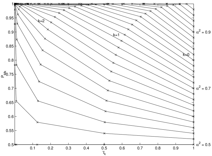
Each of the 25 lines in Fig 4 refers to a different value of , for from up to in steps of . The initial state, , when , occurs with probability , and is marked on the right-hand side of Fig 4 for each of the 25 lines. After one amplification step, , and another 25 points are marked on the graph to the left of the points for , indicating that a successful amplification step has occurred with probability . Similarly points for , ,..etc are marked successively to the left on Fig 4. The -axis shows the ML advantage, , which can be achieved with probability after steps for each value of . For instance, when , then an ML advantage of can be ensured after steps, and this can be achieved with probability given independently prepared qubits, all in state . Amplification is more rapid if already has significant ML advantage (i.e. when is high). In contrast if then no amplification of that qubit is possible. This is quite reasonable as, in this case, both states and are equally likely, so there is no ML state. Successive measurement of zero of all second qubits of each qubit pair self-verifies that we have obtained successful amplification. If, at any step, , the second qubit of the qubit pair is measured as one then amplification fails and the graph local to this qubit which has been successfully entangled up until now is completely destroyed.
5 Distributed QPA on Many-Node Factor Graphs
5.1 Preliminaries
In classical systems it is desirable to implement SPA on Factor Graphs which ’tensor-approximate’ the variable space using many small-state variables (e.g. bits), linked by small-dimensional constituent functions, thereby minimising computational complexity. In quantum systems it is similarly desirable to implement QPA on Factor Graphs using many small-state variables (e.g. qubits), linked by small-dimensional constituent unitary functions. Any Quantum Computation can be decomposed into a sequence of one or two-bit ’universal’ gate unitary operations [3]555This also implies that any classical Factor Graph can be similarly decomposed. . Computational complexity is minimised by using small-dimensional unitary matrices for constituent functions. Moreover, fine granularity of the Factor Graph allows distributed node processing. This appears to be essential for large Quantum Factor Graphs to have acceptable probability of successful global evolution, as we will show. Distributed QPA allows variable nodes to evolve entanglement only with neighbouring variable nodes so that, if a local function measurement or amplification is unsuccessful, only local evolution is destroyed. Remember that local evolution is OFTEN unsuccessful, as failure occurs when a local ancillary qubit, , is measured as , or when a local amplifying qubit is measured as 1. Therefore node localities with high likelihood of successful evolution (i.e. with positively skewed input probabilities) are likely to evolve first. These will then encourage other self-contradictory node localities to evolve successfully. In contrast, non-distributed QPA on large Factor Graphs using one large global function is very unlikely to ever succeed, especially for graphs encoding low-rate codes.

To illustrate the advangtage of distributed QPA, consider the low rate code of Fig 5, where . Both top and bottom graphs represent the code , where is a combination of XOR sub-matrices, ,, and . The top graph distributes processing. We allow and to operate independently and in parallel. Moreover, if fails to establish, then it does not destroy any successful evolution of , as the two localities are not currently entangled. Once both and have completed successfully, the subsequent probability of successful completion of is, in general, likely to increase. So distributing QPA increases likelihood of successful evolution of the complete Factor Graph. We now demonstrate this graphically. Let qubits of Fig 5 initially be in states , , , , where, for notational convenience, we assume all values are real. Then , . The probability of successful completion of is , and probability of successful completion of is . Therefore the probability of successful completion of both and after exactly parallel attempts (no less) is,
Given successful completion of and , the probability of subsequent successful completion of is,
Therefore the probability of successful completion of and , immediately followed by successful completion of is, , and the probability of successful completion of and , immediately followed by completion failure of is, . Therefore the probability of successful completion after exactly steps of and in parallel, followed by , is,
where is the set of unordered partitions of . Therefore the probability of successful completion after at most steps of and in parallel, followed by , is,
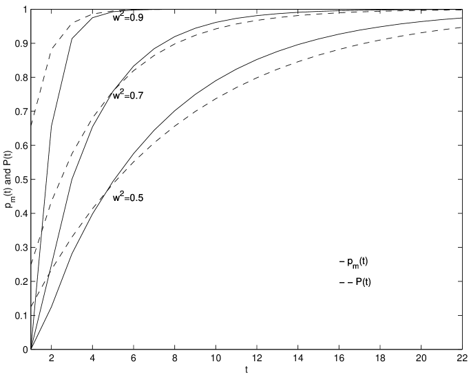
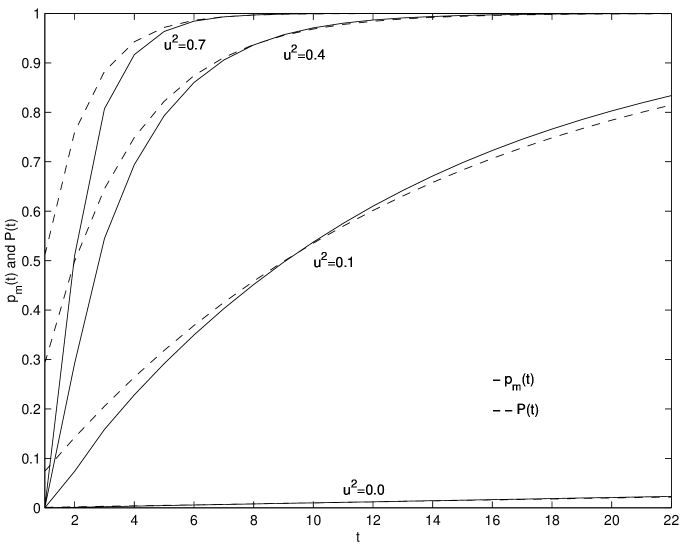
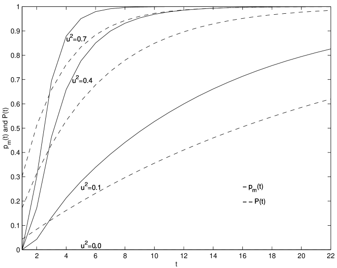
In contrast, for non-distributed QPA, the probability of successful completion, after at most steps, of , (the bottom graph of Fig 5) is . Figs 6 and 7 show plots of and versus for as varies, and as varies, respectively. For Fig 7, low values of indicate a contradiction between and the other three variables. In particular the contradiction is so pronounced when that successful QPA completion is highly unlikely. More generally, this indicates that severe internal Factor Graph contradictions are fatal to QPA (as they are for SPA). Both Fig 6 and 7 indicate that, due to initial latency of distributed processing, non-distributed QPA appears marginally faster for the first few steps. However, after a few steps distributed QPA in general becomes marginally faster. In fact results are unfairly biased towards the non-distributed case, as it is assumed that attempts to complete and have the same space-time-complexity cost, whereas is far more costly. Hence, even for this smallest example, Distributed QPA outperforms non-Distributed QPA.
The example of Fig 5 only achieves marginal advantage using Distributed QPA because the example has so few nodes. The advantage is more pronounced in Fig 8.

Fig 8 represents the code 666This code is trivial but demonstrates a ’worst-case’ low-rate scenario. In general, codes of higher rate, with or without cycles, decode more quickly. , where . We allow , , and to operate independently and in parallel. If fails to establish, then it does not destroy any successful evolution of or , as the three localities are not currently entangled. Once , , and have completed successfully, the probability of successful subsequent completion of is, in general, amplified. Let qubits of Fig 8 initially be in states , where, for notational convenience, we assume all values are real. Then , . Let the probability of successful completion after at most steps of , , and in parallel, followed by , be , and the probability of successful completion, after at most steps, of a non-distributed version of Fig 8 be . Appendix A derives and for this case. Figs 9 and 10 show plots of and versus for , , as varies, and , , , as varies, respectively. For Fig 10 low values of indicate contradiction between and the other eight qubits. The contradiction is so pronounced when that successful QPA completion is highly unlikely.
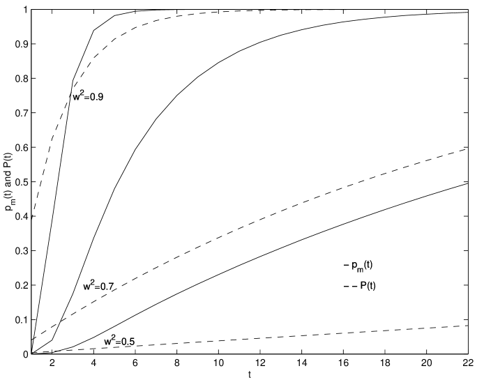
Figs 11 and 12 show plots of and versus for , , , and , , , respectively, as varies. Both figures indicate contradictions between two qubits and the rest, but the scattered nature of contradictions for Fig 12 ( and are connected to different local functions) enhances Distributed QPA performance compared to Fig 11.
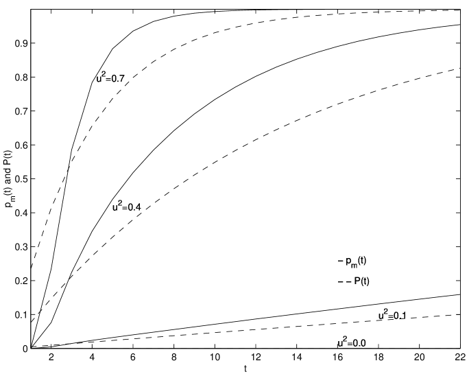
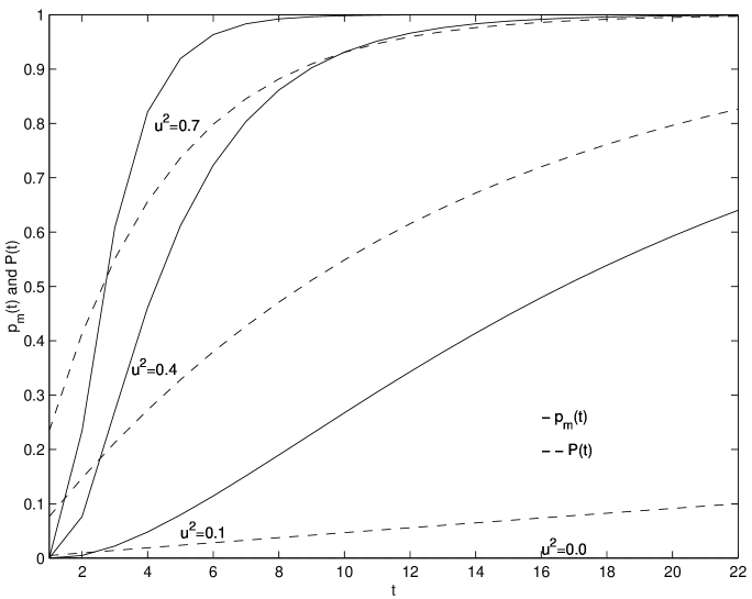
Figs 6-12 indicate that distributed QPA completes significantly faster than non-distributed QPA, in particular for cases requiring many steps, . Even more so as the presented results are unfairly biased towards the non-distributed case, as it is assumed that attempts to complete non-distributed or each constituent have the same space-time-complexity cost, whereas is far more costly. We conclude that Distributed QPA is essential for large Quantum Factor Graphs.
5.2 Free-Running Distributed QPA
Consider the notional Factor Graph of Fig 13. Each (square) function node activates time-independently on its local (circular) variable nodes. Functions successfully completed are marked with an ’X’. After a certain time, say, three ’areas of success’ evolve, due to general agreement between input variable states at these localities. This means that variables on the perimeter of each region of success are ’encouraged’ to agree with the ’general view’ of the associated region of success. Unfortunately, in the bottom left of the graph is a variable (dark circle) which strongly contradicts with the rest of the graph. No area of success evolves around it, and it is difficult for other areas of success to ’swallow’ it. Assuming the contradiction is not too strong then, eventually, after numerous attempts, the complete graph is marked with ’X’s and the Graph evolves successfully. At this point the contents of each qubit variable can be amplified, and final measurement of all qubits provides the ML codeword with high probability. The advantage of a free-running strategy, where each function node is free to activate asynchronously, is that regions of general agreement develop first and influence other areas of the graph to ’follow their opinion’. Fig 13 also shows that one ’bad’ (contradictory) qubit can be a fatal stumbling block to successful evolution of the whole graph (as it can for SPA on classical graphs). Thus Distributed QPA requires Fault-Tolerance, where only an arbitrary subset of entangled nodes are required as a final result (node redundancy). The free-running schedule of Fig 13 naturally avoids the ’bad’ qubits, but sufficient evolution occurs when enough function nodes complete. Alternatively, bad qubits could be set to after a time-out. A more detailed proposal of Fault-Tolerant QPA is left for future work.
Fig 13 also serves to illustrate the ’template’ for a Reconfigurable Quantum Graph Array. One can envisage initialising an array of quantum variables so that two local variables can be strongly or weakly entangled by identifying the mutual square function nodes with strongly or weakly-entangling matrices, respectively. In particular, two neighbouring nodes may be ’locally disconnected’ by setting the function node joining them to a tensor-decomposable matrix, (i.e. zero-entangling). The quantum computer is then measurement-driven. The concept of measurement-driven quantum computation has also recently been pursued in [8], where a uniform entanglement is set-up throughout the array 777It is interesting that this entanglement is strongly related to Rudin-Shapiro and quadratic constructions [7] prior to computation via measurement.

Fig 14 shows the system view of QPA. A continual stream of pure qubits needs to be initialised and then entangled, and then amplified, so as to ensure at least one successful entangled and amplified output from the whole apparatus.

6 Phase QPA
The above discussions have ignored the capacity of Quantum Systems to carry phase information. In fact QPA, as presented so far, is immune to phase modification, as classical probabilities have no phase component. However QPA should be generalised to cope with phase shift in order to decode quantum information. This is the subject of ongoing research.
7 Conclusion and Discussion
The Quantum Product Algorithm (QPA) on a Factor Graph has been presented for Maximum-Likelihood (ML) Decoding of Classical ’soft’ information using quantum resources. The relationship of QPA to the Sum-Product Algorithm (SPA) has been indicated, where avoidance of summary allows QPA to overcome small graph cycles. Quantum Factor Graphs use small unitary matrices which each act on only a few qubits. QPA is measurement-driven and is only statistically likely to succeed after many attempts. The ML codeword is obtained with maximum likelihood by measuring the entangled vector resulting from successful QPA. To ensure a high probability of measuring the ML codeword QPA output can be amplified prior to measurement. The complete ML decoder is only successful after many attempts. Finally, free-running Distributed QPA is proposed to improve the likelihood of successful QPA completion. The free-running distributed structure suggests further benefit will be obtained by introducing Fault-Tolerance in the form of redundant function and variable nodes. Phase aspects of QPA have yet to be explored. This paper has been written to demonstrate the exponential capacity of quantum systems, and their natural suitability for graph decompositions such as the Factor Graph. The paper has not tried to deal with quantum noise and quantum decoherence, but one can expect the Factor Graph form to ’gracefully’ expand to cope with the extra redundancy necessary to protect qubits from decoherence and noise. When viewed in the context of entangled space, it is surprising how successful classical message-passing algorithms are, even though they are restricted to operate in tensor product space. This suggests that methods to improve the likelihood of successful QPA completion may include the possibility of hybrid QPA/SPA graphs, where SPA operates on non-cyclic and resolvable parts of the graph, leaving QPA to cope with small cycles or unresolved areas of the graph.
8 Appendix A - Deriving and for Fig 8
The probability of successful completion of , is , and similarly for and . Let , , . Then the probability of successful completion of , , and after exactly parallel attempts is,
Given successful completion of , , and , the probability of subsequent successful completion of is,
Therefore the probability of successful completion of , , and , immediately followed by successful completion of is, , and the probability of successful completion of , , and , immediately followed by completion failure of is, . The probability of successful completion after exactly steps of , , and in parallel, followed by , is,
where is the set of unordered partitions of . Therefore the probability of successful completion after at most steps of , , and in parallel, followed by , is,
In contrast, the probability of successful completion, after at most steps, of a non-distributed version of Fig 8 is .
References
- [1] AJI (S.M.), McELIECE (R.J.), ”The Generalized Distributive Law”, IEEE Trans. Inform. Theory, Vol. IT-46, pp. 325-343, March 2000
- [2] BERROU (C.),GLAVIEUX (A.),THITIMAJSHIMA (P.), ”Near Shannon-Limit Error-Correcting Coding and Decoding: Turbo-Codes”, Proc. 1993 IEEE Int. Conf. on Communications (Geneva, Switzerland),, pp. 1064-1070, 1993
- [3] DiVINCENZO (D.P.), ”Two-Bit Gates are Universal for Quantum Computation”, Phys. Rev. A 51, Vol 1015, 1995, Also LANL arXiv:cond-mat/9407022
- [4] GALLAGER (R.G.), ”Low Density Parity Check Codes,” IRE Trans. Inform. Theory, Vol IT-8, pp 21-28, Jan. 1962
- [5] KSCHISCHANG (F.R.),FREY (B.J.),LOELIGER (H-A.), ”Factor Graphs and the Sum-Product Algorithm,” IEEE Trans. Inform. Theory, Vol 47, No 2, pp 498-519, Feb. 2001
- [6] MACKAY (D.J.C.),NEAL (R.M.), ”Near Shannon Limit Performance of Low Density Parity Check Codes,” Electronics Letters, Vol 32, No 18, pp 1645-1646, Aug 1996. Reprinted Vol 33, No 6, pp 457-458, Mar 1997
- [7] PARKER (M.G.), RIJMEN (V.), ”The Quantum Entanglement of Bipolar Sequences”, Sequences and their Applications, SETA’01, Bergen, Norway, 13-17 May, 2001 Also http://www.ii.uib.no/matthew/MattWeb.html
- [8] RAUSSENDORF (R.),BRIEGEL (H.J.), ”Quantum Computing via Measurements Only”, LANL arXiv:quant-ph/0010033, 7 Oct 2000
- [9] SHOR (P.W.), ”Polynomial-Time Algorithms for Prime Factorization and Discrete Logarithms on a Quantum Computer”, SIAM J. Computing, Vol 26, pp 1484-, 1997 First appeared in Proceedings of the Annual Symposium on the Theory of Computer Science, ed. S. Goldwasser, IEEE Computer Society Press, Los Alamitos, CA, pp 124-, 1994, Expanded Version: LANL: quant-ph/9508027
- [10] STEANE (A.M.), ”Quantum Computing,” Rept.Prog.Phys., Vol 61, pp 117-173, 1998, Also LANL: quant-ph/9708022
- [11] TUCCI (R.R.), ”How to Compile a Quantum Bayesian Net”, LANL: quant-ph/9805016, 7 May, 1998
- [12] TUCCI (R.R.), ”Quantum Information Theory - A Quantum Bayesian Net Perspective”, LANL: quant-ph/9909039, 13 Sep, 1999