Abstract
We investigate correlations between fluorescence photons emitted by single N-V centers in diamond with respect to the optical excitation power. The autocorrelation function shows clear photon antibunching at short times, proving the uniqueness of the emitting center. We also report on a photon bunching effect, which involves a trapping level. An analysis using rate-equations for the populations of the N-V center levels shows the intensity dependence of the rate equation coefficients.
Bunching and antibunching from single NV color centers in diamond
Introduction
Quantum cryptography relies on the fact that single quantum states can not be cloned. In this way coding information on single photons would ensure a secure transmission of encryption keys. First attempts for quantum cryptography systems [1, 2] were based on attenuated laser pulses. Such sources can actually produce isolated single photons, but the poissonian distribution of the photon number does not guarantee both the uniqueness of the emitted photon and a high bit-rate. Therefore a key milestone for efficient and secure quantum cryptography systems is the development of single photon sources.
Several pioneering experiments have already been realized in order to obtain single photon sources. Among these attempts one can cite twin-photons experiments [3, 4], coulomb blockade of electrons in quantum confined heterojunctions [5], or fluorescence emission from single molecules [6, 7]. Up to now interesting results were obtained, but considerable work is still needed to design a reliable system, working at room temperature with a good stability and well-controlled emission properties. More recently several systems have been proven to be possible candidates for single photon sources. Antibunching was indeed observed in CdSe nanospheres [8], thereby proving the purely quantum nature of the light emitted by these sources. In the same way photon antibunching in Nitrogen-Vacancy (N-V) colored centers in diamond was reported by our group [9] and by Kurtsiefer et al [10]. A remarkable property of these centers is that they do not photobleach at room temperature: the fluorescence level remains unchanged after several hours of continuous laser irradiation of a single center in the saturation regime. These centers are therefore very promising candidates for single photon sources.
In this paper we present further investigation of the fluorescence light emitted by NV colored centers. We analyze the system dynamic through the measurement of the autocorrelation function, showing the existence of a shelving effect which reduces the counting rate of the fluorescence emission, and gives rise to photon bunching [11]. We study the dependence of this behavior on the pumping power, and we compare the experimental results with the predictions of a three-level model using rate equations.
1 Experimental setup
Our experimental set-up is based on a home-made scanning confocal microscope.
A CW frequency doubled Nd:YAG laser () is focused on the sample by a high numerical aperture () immersion objective. A PZT-mounted mirror allows a x-y scan of the sample, and a fine z-scan is obtained using another PZT.
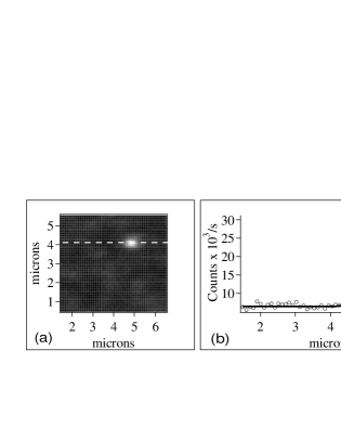
The sample is a crystal of synthetic Ib diamond from Drukker International. The Nitrogen-Vacancy centers consist in a substitutional nitrogen with an adjacent vacancy, and are found with a density of about 1 m-3 in Ib diamond. The centers can be seen with a signal to background ratio of about by scanning the sample as shown in figure 1, and a computer-controlled servo-loop allows to focus on one center for hours.
The fluorescence is collected by the same objective, and separated from excitation light by a dichroic mirror. High rejection () high-pass filters remove any leftover pump light. Spatial filtering is achieved by focusing on a pinhole. The fluorescence is then analyzed by an ordinary Hanbury-Brown and Twiss set-up. The time delay between the two photons is converted by a time-to-amplitude converter (TAC) into a voltage which is digitalized by a computer board.
In a low counting regime, this system allows us to record the autocorrelation function: .
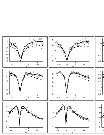
Experimental data were corrected from background noise, and normalized to the coincidence number corresponding to a poissonian source of equivalent power [9]. Different correlation functions obtained for several pumping power are shown in figure 2. These functions are centered around , but one can notice slight drifts attributed to thermal drift of our acquisition electronics. For , goes clearly down to zero, which is the signature of a single emitting dipole. On the other hand, goes beyond 1 at longer times, and then decays to 1. This behavior is an evidence of the presence of a trapping level. To correctly describe the system we therefore considered a 3-level system.
2 Theoretical background and discussion
Owing to the fast damping of coherences, we use rate equations. Let us consider the 3-level scheme described in figure 3.

The evolution of the populations are therefore given by:
| (1) |
with the initial condition , at , which means that a photon has just been emitted and the system is therefore prepared in its ground state. The decay rate from level 3 to 1 is neglected [12].
By analytically solving equations 1, one can derive
| (2) |
with the stationary population:
| (3) |
and with
| (4) |
| (5) |
| (6) |
We thus have four equations which enables us to express the four rates with respect to the experimental variables . By fitting the experimental values of with expression 2 we obtain the values of , and for each value of the intensity. The last value needed in order to solve the system concerns the parameter which is directly linked to the count rate
| (7) |
We assume that doesn’t depend on the pump power, and we set to the value for which this condition is satisfied. We found which is in perfect agreement with our estimated value [9]. The parameters are plotted as functions of pumping power in figure 4.
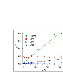
Note that is, as expected, a linear function of the pumping power, and that has a constant value of 11.6ns, which corresponds to results reported in literature [13].
What is noteworthy here is that and linearly depend on pump power, with greater than , which means that at high pumping power the system tends to be shelved into the third level. This intensity-dependent effect has not been reported yet. In Figure 2, three plots were superimposed to the experimental results. The solid line represents the best fit. The dashed line represents the result of equation 2 with values of and independent on intensity taken from reference [10]. One can see in this last case that the agreement between calculated and experimental value is not fully satisfactory. Finally, the thin line is obtained by using the values of and given by the linear fit of figure 4. Agreement with the experimental results is good.
This intensity dependence of and can also be observed on the total photon counts. In fact the number of photons emitted per second should decrease as the trapping in the metastable state increases.
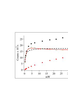
Figure 5 shows the count rate of the single N-V center as a function of the pump power. We clearly see a decrease in the photon counts. We can fit with a good agreement our experimental data using equations 7 and 3.
We have repeated this experiment with the Nd:YAG line and the Argon line and found similar linear dependency of the and rates with the pump power.
Conclusion
We have measured the autocorrelation function of the fluorescence light emitted from a single NV colored center in diamond using a confocal microscope. Our results are in very good agreement with what can be expected from rate equations in a 3-level scheme, provided that a linear dependence of some rate coefficients with pumping power is assumed. Such an effect has not been reported yet, and must be taken into account when designing a pulsed single-photon source.
1
References
- [1] A. Muller, J. Breguet, and N. Gisin, Europhysics Letters, 23 (6), 383 (1993),
- [2] P. D. Townsend, J. G. Rarity, and P. R. Tapster, Electronics Letters, 29 (7), 634 - 635 (1993)
- [3] P. Grangier, G. Roger and A. Aspect, Europhysics Lett. 1, 173 (1986).
- [4] C. K. Hong and L. Mandel, Phys. Rev. Lett. 56, 58 (1986).
- [5] J. Kim, O. Benson, H. Kan, and Y. Yamamoto, Nature 397, 500 (1999)
- [6] F. De Martini, G. Di Giuseppe, and M. Marrocco, Phys . Rev. Lett. 76, 900 (1996).
- [7] C. Brunel, B. Lounis, P. Tamarat, and M. Orrit, Phys. Rev. Lett. 83, 2722 (1999).
- [8] P. Michler, A. Imamoglu; MD. Mason, P. J. Carson, G.F. Strouse, S.K. Buratto, Nature 406, 968 (2000)
- [9] R. Brouri, A. Beveratos, J.-Ph. Poizat, Ph. Grangier, Opt. Lett. 25(17), 1294 (2000).
- [10] C. Kurtsiefer, S. Mayer, P. Zarda, and Harald Weinfurter, Phys. Rev. Lett. 85(2), 290 (2000).
- [11] J. Bernard, L. Fleury, H. Talon, M. Orrit, Journal of Chemical Physics 98 (2), 850 (1993).
- [12] A. Dräbenstedt, L. Fleury, C Tietz, F. Jelezko, S. Kilin, A. Nizovtev, and J. Wrachtrup, Phys. Rev. B 60, 11503 (1999).
- [13] A. T. Collins, M. F. Thomaz, and M. I. B. Jorge, J. Phys. C: Solid State Phys. 16, 2177 (1983).