Entanglement of Formation
and
Conditional Information Transmission

Abstract

We show that the separability of states in quantum mechanics has a close counterpart in classical physics, and that conditional mutual information (a.k.a. conditional information transmission) is a very useful quantity in the study of both quantum and classical separabilities. We also show how to define entanglement of formation in terms of conditional mutual information. This paper lays the theoretical foundations for a sequel paper which will present a computer program that can calculate a decomposition of any separable quantum or classical state.

1 Introduction

Recently, a few authors[1][2][3] have noticed a deep connection between conditional mutual information and quantum separability. In a parallel development, some researchers[4][5] have recently proven theorems giving necessary and sufficient conditions for quantum separability using ideas that hark back to a paper by Hughston-Jozsa-Wootters[6]. An important goal of this paper is to tie together these two apparently disconnected lines of thought.

In this paper, we explore the classical roots of quantum entanglement. We show that the separability of states in quantum mechanics has a close counterpart in classical physics, and that conditional mutual information is a very useful quantity in the study of both quantum and classical separabilities.

In this paper, we also show how to define entanglement of formation in terms of conditional mutual information.

In a sequel paper that will soon follow, we will present a computer program based on the theory of this paper. Our software uses a relaxation algorithm to calculate a decomposition of any separable quantum or classical state. The authors of Ref.[4] have written some excellent software that can calculate similar things using an algorithm different from ours.

2 Notation

In this section, we will introduce certain notation which is used throughout the paper.

For any finite set $S$, let $|S|$ denote the number of elements in $S$. The Kronecker delta function $\delta(x,y)$ equals one if $x=y$ and zero otherwise. We will often abbreviate $\delta(x,y)$ by $\delta^{x}_{y}$. For any Hilbert space ${\cal H}$, $dim({\cal H})$ will stand for the dimension of ${\cal H}$. If $|\psi\rangle\in{\cal H}$, then we will often represent the projection operator $|\psi\rangle\langle\psi|$ by $\pi(\psi)$.

We will underline random variables. For example, we might write $P({\underline{x}}=x)$ for the probability that the random variable ${\underline{x}}$ assumes value $x$. $P({\underline{x}}=x)$ will often be abbreviated by $P(x)$ when no confusion will arise. $S_{\underline{x}}$ will denote the set of values which the random variable ${\underline{x}}$ may assume, and $N_{\underline{x}}$ will denote the number of elements in $S_{\underline{x}}$. With each random variable ${\underline{x}}$, we will associate an orthonormal basis $\{|x\rangle|x\in S_{\underline{x}}\}$ which we will call the ${\underline{x}}$ basis. We will represent by ${\cal H}_{\underline{x}}$ the Hilbert space spanned by the ${\underline{x}}$ basis. Thus, $dim{\cal H}_{{\underline{x}}}=N_{\underline{x}}$.

For any two random variables ${\underline{x}}$ and ${\underline{y}}$, $S_{{\underline{x}},{\underline{y}}}$ will represent the direct product set $S_{\underline{x}}\times S_{\underline{y}}=\{(x,y)|x\in S_{\underline{x}},y\in S_{\underline{y}}\}$. Furthermore, ${\cal H}_{{\underline{x}},{\underline{y}}}$ will represent ${\cal H}_{\underline{x}}\otimes{\cal H}_{\underline{y}}$, the tensor product of Hilbert spaces ${\cal H}_{\underline{x}}$ and ${\cal H}_{\underline{y}}$. If $|x\rangle$ for all $x$ is the ${\underline{x}}$ basis and $|y\rangle$ for all $y$ is the ${\underline{y}}$ basis, then ${\cal H}_{{\underline{x}}{\underline{y}}}$ is the vector space spanned by $\{|x,y\rangle|x\in S_{\underline{x}},y\in S_{\underline{y}}\}$, where $|x,y\rangle=|x\rangle|y\rangle$.

For any $|\psi_{\underline{x}}\rangle\in{\cal H}_{\underline{x}}$, we will use $\psi_{x}$ to represent $\langle x|\psi_{\underline{x}}\rangle$. For any $|\psi_{{\underline{x}}{\underline{y}}}\rangle\in{\cal H}_{{\underline{x}}{\underline{y}}}$, we will use $\psi_{xy}$ to represent $\langle x,y|\psi_{{\underline{x}}{\underline{y}}}\rangle$.

${\rm pd}(S_{\underline{x}})$ will denote the set of all probability distributions $P(\cdot)$ for the random variable ${\underline{x}}$; i.e., all functions $P:S_{\underline{x}}\rightarrow[0,1]$ such that $\sum_{x}P(x)=1$. ${\rm dm}({\cal H}_{{\underline{x}}})$ will denote the set of all density matrices acting on the Hilbert space ${\cal H}_{{\underline{x}}}$; i.e., the set of all $N_{\underline{x}}$ dimensional Hermitian matrices with unit trace and non-negative eigenvalues.

Whenever we use the word “ditto”, as in “X (ditto, Y)”, we mean that the statement is true if X is replaced by Y. For example, if we say “A (ditto, X) is smaller than B (ditto, Y)”, we mean “A is smaller than B” and “X is smaller than Y”.

This paper will also utilize certain notation associated with classical and quantum entropy. See Ref.[7] for definitions and examples of the use of such notation.

3 Classical Separability

In this section, we will discuss classical separability. In the next section, we will discuss quantum separability, stressing the similarities with the classical case.

We will say $P(x,y)\in{\rm pd}(S_{{\underline{x}}{\underline{y}}})$ is $N$-separable iff there exists some random variable ${\underline{\alpha}}$ with $N_{\underline{\alpha}}=N$ and there exist probability distributions $\tilde{P}(x|\alpha)\in{\rm pd}(S_{\underline{x}})$, $\tilde{P}(y|\alpha)\in{\rm pd}(S_{\underline{y}})$, $\tilde{P}(\alpha)\in{\rm pd}(S_{\underline{\alpha}})$ such that $P(x,y)$ can be “decomposed” thus:

$$P(x,y)=\sum_{\alpha}\tilde{P}(x|\alpha)\tilde{P}(y|\alpha)\tilde{P}(\alpha)\;.$$ (1)

We will also say that $P(x,y)\in{\rm pd}(S_{{\underline{x}}{\underline{y}}})$ is separable iff it is $N$-separable for some $N$.

Theorem 3.1

$P(x,y)\in{\rm pd}(S_{{\underline{x}}{\underline{y}}})$ is $N$-separable (ditto, separable) if and only if there exists $\tilde{P}(x,y,\alpha)\in{\rm pd}(S_{{\underline{x}}{\underline{y}}{\underline{\alpha}}})$ with $N_{\underline{\alpha}}=N$ (ditto, with $N_{\underline{\alpha}}$ arbitrary) such that

$$P(x,y)=\sum_{\alpha}\tilde{P}(x,y,\alpha)\;$$ (2)

and

$$\tilde{P}(x,y,\alpha)\tilde{P}(\alpha)=\tilde{P}(x,\alpha)\tilde{P}(y,\alpha)\;$$ (3)

for all $(x,y,\alpha)\in S_{{\underline{x}}{\underline{y}}{\underline{\alpha}}}$. (The last condition is just another way of expressing conditional independence:

$$\tilde{P}(x,y|\alpha)=\tilde{P}(x|\alpha)\tilde{P}(y|\alpha)\;.$$ (4)

)

proof:

($\Rightarrow$) Since $P(x,y)$ is separable, there exist probability distributions $\tilde{P}(x|\alpha)$, $\tilde{P}(y|\alpha)$, $\tilde{P}(\alpha)$. Define $\tilde{P}(x,y,\alpha)\in{\rm pd}(S_{{\underline{x}}{\underline{y}}{\underline{\alpha}}})$ by $\tilde{P}(x,y,\alpha)=\tilde{P}(x|\alpha)\tilde{P}(y|\alpha)\tilde{P}(\alpha)$ $\tilde{P}(x,y,\alpha)$ clearly satisfies all the conditions imposed upon it by the right hand side of the theorem.

($\Leftarrow$) The right hand side of the theorem provides us with $\tilde{P}(x,y,\alpha)\in{\rm pd}(S_{{\underline{x}}{\underline{y}}{\underline{\alpha}}})$. We can use it to construct conditional probabilities $\tilde{P}(x|\alpha)$, $\tilde{P}(y|\alpha)$ and $\tilde{P}(\alpha)$ which satisfy Eq.(1). QED

Suppose $f(x,y)$ is a real valued function of two arguments $x,y$ (i.e., $f:S_{\underline{x}}\times S_{\underline{y}}\rightarrow R$). Let $*$ stand for either addition or multiplication. If there exist real valued functions $f_{1}(x)$ and $f_{2}(y)$ such that $f(x,y)=f_{1}(x)*f_{2}(y)$ for all $x,y$, then we will say that $f$ is an x, y *corrugated surface.

Suppose that $f(x,y)=f_{1}(x)*f_{2}(y)$ is a *corrugated surface such that the functions $f_{1},f_{2}$ are differentiable. Suppose the z axis points upward, the x axis eastward, and the y axis northward. If we plot $f(x,y)$ along the z direction, then the mountain tops and valley bottoms of the $f$ surface are all oriented along either the east-west or the north-south directions. Indeed, if at $x=x_{0}$, $\partial_{x}f_{1}(x_{0})=0$, then $\partial_{x}f(x_{0},y)=0$ for all $y$; and likewise if $\partial_{y}f_{2}(y_{0})=0$, then $\partial_{y}f(x,y_{0})=0$ for all $x$. This is true regardless of whether * stands for multiplication or addition.

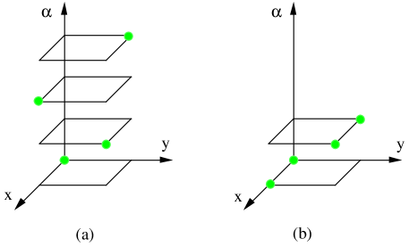
Figure 1: Two $(x,y,\alpha)$ lattices. Filled circles represent lattice points which have non-zero probability.

Now consider any $\tilde{P}(x,y,\alpha)\in{\rm pd}(S_{{\underline{x}}{\underline{y}}{\underline{\alpha}}})$. If $\tilde{P}(x,y,\alpha)$ satisfies Eq.(3), then it is an $x,y$ product-corrugated surface at fixed $\alpha$. One can convey this concept graphically by drawing a 3-dimensional orthogonal lattice with main axes $x,y,\alpha$, and writing at each lattice point $(x,y,\alpha)\in S_{{\underline{x}}{\underline{y}}{\underline{\alpha}}}$ the value $\tilde{P}(x,y,\alpha)$. Each $\alpha\in S_{\underline{\alpha}}$ determines a different horizontal plane. The values of $\tilde{P}(x,y,\alpha)$ at each horizontal plane are product-corrugated. This geometrical insight immediately suggest that all $P(x,y)\in{\rm pd}(S_{{\underline{x}}{\underline{y}}})$ are separable. Two possible decompositions of $P(x,y)$ are as follows:

($a$) Suppose that $N_{\underline{\alpha}}=N_{\underline{x}}N_{\underline{y}}$ and each $\alpha$ plane has a single lattice point $(x_{\alpha},y_{\alpha})$ with non-zero probability. Furthermore, suppose that the point with non-zero probability is different for each $\alpha$ plane (i.e., $(x_{\alpha_{1}},y_{\alpha_{1}})\neq(x_{\alpha_{2}},y_{\alpha_{2}})$ iff $\alpha_{1}\neq\alpha_{2}$.) See Fig.(1a) for an example with $N_{\underline{x}}=N_{\underline{y}}=2$. Let $\alpha(x,y)$ be a 1-1 onto function which maps $S_{{\underline{x}}{\underline{y}}}\rightarrow S_{{\underline{\alpha}}}$ and $(x_{\alpha},y_{\alpha})\rightarrow\alpha$. Define $\tilde{P}(\cdot)$ by

$$\tilde{P}(x,y,\alpha)=P(x,y)\delta(\alpha,\alpha(x,y))=P(x_{\alpha},y_{\alpha})\delta(x,x_{\alpha})\delta(y,y_{\alpha})\;.$$ (5)

It is easy to check that $\tilde{P}(\cdot)$ is an element of ${\rm pd}(S_{{\underline{x}}{\underline{y}}{\underline{\alpha}}})$ that satisfies Eqs. (2) and (3).

($b$) Suppose that $N_{\underline{\alpha}}=N_{\underline{y}}$ and at each $\alpha$ plane all lattice points have zero probability except for possibly those in a line of lattice points $L_{\alpha}=\{(x,y_{\alpha})|x\in S_{\underline{x}}\}$. Furthermore, suppose $L_{\alpha_{1}}\neq L_{\alpha_{2}}$ iff $\alpha_{1}\neq\alpha_{2}$. See Fig.(1b) for an example with $N_{\underline{x}}=N_{\underline{y}}=2$. Let $\alpha(y)$ be a 1-1 onto function which maps $S_{{\underline{y}}}\rightarrow S_{{\underline{\alpha}}}$ and $y_{\alpha}\rightarrow\alpha$. Define $\tilde{P}(\cdot)$ by

$$\tilde{P}(x,y,\alpha)=P(x,y)\delta(\alpha,\alpha(y))=P(x,y_{\alpha})\delta(y,y_{\alpha})\;.$$ (6)

It is easy to check that this $\tilde{P}(\cdot)$ is an element of ${\rm pd}(S_{{\underline{x}}{\underline{y}}{\underline{\alpha}}})$ that satisfies Eqs. (2) and (3).

Note that even though every $P(x,y)\in{\rm pd}(S_{{\underline{x}}{\underline{y}}})$ is separable, it may not be $N$-separable. Example ($b$) above implies that $P(x,y)$ is $N_{\underline{\alpha}}$ separable when $N_{\underline{\alpha}}\geq min(N_{\underline{x}},N_{\underline{y}})$, but what if $N_{\underline{\alpha}}$ is smaller than this? (for example, if $N_{\underline{\alpha}}=2$ but $N_{\underline{x}},N_{\underline{y}}>>2$). For small enough $N_{\underline{\alpha}}$, it may be impossible to construct a $\tilde{P}(x,y,\alpha)$ that satisfies all the constraints given by Eqs. (2) and (3).

For $P(x,y)\in{\rm pd}(S_{{\underline{x}}{\underline{y}}})$ and any integer $N\geq 1$, define

$$E^{(N)}_{F}(P)=\frac{1}{2}\min_{\tilde{P}}H({\underline{x}}:{\underline{y}}|{\underline{\alpha}})\;,$$ (7)

where the minimum is taken over the set of all $\tilde{P}(x,y,\alpha)\in{\rm pd}(S_{{\underline{x}}{\underline{y}}{\underline{\alpha}}})$ such that $N_{\underline{\alpha}}=N$ and $P(x,y)=\sum_{\alpha}\tilde{P}(x,y,\alpha)$. The conditional mutual entropy $H({\underline{x}}:{\underline{y}}|{\underline{\alpha}})$ is calculated for the probability distribution $\tilde{P}$.

Theorem 3.2

$P(x,y)\in{\rm pd}(S_{{\underline{x}}{\underline{y}}})$ is $N$-separable if and only if $E^{(N)}_{F}(P)=0$.

proof:

($\Rightarrow$) Clear.

($\Leftarrow$) There exists a $\tilde{P}(x,y,\alpha)\in{\rm pd}(S_{{\underline{x}}{\underline{y}}{\underline{\alpha}}})$ such that $N_{\underline{\alpha}}=N$, $P(x,y)=\sum_{\alpha}\tilde{P}(x,y,\alpha)$, and $H({\underline{x}}:{\underline{y}}|{\underline{\alpha}})=0$. Because this conditional mutual entropy vanishes, $\tilde{P}(x,y|\alpha)=\tilde{P}(x|\alpha)\tilde{P}(y|\alpha)$. Hence, $P(x,y)$ is $N$-separable. QED

4 Quantum Separability

We say $\rho\in{\rm dm}({\cal H}_{{\underline{x}}{\underline{y}}})$ is $N$-separable (ditto, separable) iff there exist a random variable ${\underline{\mu}}$ with $N_{\underline{\mu}}=N$ (ditto, with arbitrary $N_{\underline{\mu}}$) and there exist $P(\mu)\in{\rm pd}(S_{\underline{\mu}})$, $\rho_{\underline{x}}^{\mu}\in{\rm dm}({\cal H}_{{\underline{x}}})$ and $\rho_{\underline{y}}^{\mu}\in{\rm dm}({\cal H}_{{\underline{y}}})$ such that $\rho$ can be “decomposed” thus:

$$\rho=\sum_{\mu}P(\mu)\rho_{\underline{x}}^{\mu}\rho_{\underline{y}}^{\mu}\;.$$ (8)

An equivalent definition is: $\rho\in{\rm dm}({\cal H}_{{\underline{x}}{\underline{y}}})$ is $N$-separable (ditto, separable) iff there exist a random variable ${\underline{\alpha}}$ with $N_{\underline{\alpha}}=N$ (ditto, with arbitrary $N_{\underline{\alpha}}$) and there exist $w_{\alpha}\in pd(S_{\underline{\alpha}})$, $|\psi^{\alpha}_{\underline{x}}\rangle\in{\cal H}_{{\underline{x}}}$ and $|\psi^{\alpha}_{\underline{y}}\rangle\in{\cal H}_{{\underline{y}}}$ such that $\rho$ can be “decomposed” thus:

$$\rho=\sum_{\alpha}w_{\alpha}\pi(\psi^{\alpha}_{\underline{x}})\pi(\psi^{\alpha}_{\underline{y}})\;.$$ (9)

The second definition clearly implies the first. To see that the first definition implies the second: for each $\mu$, express $\rho_{\underline{x}}^{\mu}$ and $\rho_{\underline{x}}^{\mu}$ in terms of their eigenstates:

$$\rho_{\underline{x}}^{\mu}=\sum_{a}P(a|\mu)|\phi^{\mu a}_{\underline{x}}\rangle\langle\phi^{\mu a}_{\underline{x}}|\;,$$ (10)

$$\rho_{\underline{y}}^{\mu}=\sum_{b}P(b|\mu)|\phi^{\mu b}_{\underline{y}}\rangle\langle\phi^{\mu b}_{\underline{y}}|\;.$$ (11)

We identify the index $\alpha$ with the 3-tuple $(\mu,a,b)$ so $S_{\underline{\alpha}}=S_{{\underline{\mu}}{\underline{a}}{\underline{b}}}$. We define for all $\alpha\in S_{\underline{\alpha}}$:

$$w_{\alpha}=P(a|\mu)P(b|\mu)P(\mu)\;,$$ (12)

$$|\psi^{\alpha}_{\underline{x}}\rangle=|\phi^{\mu a}_{\underline{x}}\rangle\;$$ (13)

(note that the right hand side is the same for all $b$), and

$$|\psi^{\alpha}_{\underline{y}}\rangle=|\phi^{\mu b}_{\underline{y}}\rangle\;$$ (14)

(note that the right hand side is the same for all $a$). With these definitions, Eq.(9) follows.

In the previous section about classical separability, we encountered several theorems of the form: “$P$ is separable iff condition X”. These theorems had matching theorems of the form “$P$ is $N$-separable iff $N=N_{\underline{\alpha}}$ and condition X”. In what follows, we will often encounter theorems of the form: “$\rho$ is separable iff condition X”. As in the classical case, these theorems about separability have obvious matching theorems about $N$-separability (“$\rho$ is $N$-separable iff $N=N_{\underline{\alpha}}$ and condition X”), but for simplicity, we will not mention them henceforth.

Consider some Hilbert space ${\cal H}$ and some $\rho\in{\rm dm}({\cal H})$. $\rho$ can be expressed as

$$\rho=\sum_{j}\lambda_{j}|\phi^{j}\rangle\langle\phi^{j}|\;,$$ (15)

where $(\lambda_{j},|\phi^{j}\rangle)$ for all $j$ are the eigenvalues and eigenvectors of $\rho$. In Ref.[6], Hughston, Jozsa and Wootters (HJW) proved the following theorem.

Theorem 4.1 (HJW)

$\rho\in{\rm dm}({\cal H})$ can be expressed as

$$\rho=\sum_{\alpha}w_{\alpha}|\psi^{\alpha}\rangle\langle\psi^{\alpha}|\;,$$ (16)

where $w_{\alpha}\in{\rm pd}(S_{\underline{\alpha}})$, and $|\psi^{\alpha}\rangle\in{\cal H}$ for all $\alpha$ if and only if there exists a transformation $T^{\alpha}_{j}$ ($\alpha\in S_{\underline{\alpha}}$, $j\in\{1,2,\ldots,dim({\cal H})\}$) which is “right unitary”:

$$\sum_{\alpha}T^{\alpha}_{j}T^{\alpha*}_{j^{\prime}}=\delta^{j^{\prime}}_{j}\;,$$ (17)

and which satisfies

$$\sum_{j}T^{\alpha}_{j}\sqrt{\lambda_{j}}|\phi^{j}\rangle=\sqrt{w_{\alpha}}|\psi^{\alpha}\rangle\;.$$ (18)

proof:

($\Leftarrow$) Multiply each side of Eq.(18) by its complex conjugate and sum over $\alpha$.

($\Rightarrow$) Using Eqs.(15) and (16) and the fact that the eigenvectors $|\phi^{j}\rangle$ are orthonormal, we get:

$$\sum_{\alpha}\sqrt{w_{\alpha}}\langle\phi^{j}|\psi^{\alpha}\rangle\langle\psi^{\alpha}|\phi^{j^{\prime}}\rangle\sqrt{w_{\alpha}}=\lambda_{j}\delta^{j^{\prime}}_{j}\;.$$ (19)

For those $j$ such that $\lambda_{j}\neq 0$, define $T$ by

$$T^{\alpha}_{j}=\sqrt{\frac{w_{\alpha}}{\lambda_{j}}}\langle\phi^{j}|\psi^{\alpha}\rangle\;.$$ (20)

One can represent $T^{\alpha}_{j}$ as a matrix with rows labelled by $j\in\{1,2,\ldots,dim({\cal H})\}$ and columns labelled by $\alpha\in S_{\underline{\alpha}}$. Eq.(20) defines only those rows of $T$ with index $j$ such that $\lambda_{j}\neq 0$. Eq.(19) tells us that those rows which are defined by Eq.(20) are orthonormal. The remaining rows of $T$ can be filled in using the Gram-Schmidt process [8]. Once $T$ is fully specified, all the rows of $T$ are orthonormal, and therefore Eq.(17) follows. It is easy to check that the $T$ we have constructed also satisfies Eq.(18). QED

The HJW Theorem refers to density matrices $\rho$ in an arbitrary Hilbert space ${\cal H}$. But what if ${\cal H}$ is a tensor product of two Hilbert spaces ${\cal H}_{{\underline{x}}}$ and ${\cal H}_{{\underline{y}}}$? Refs.[4] and [5] apply the HJW Theorem to tensor product spaces. They prove the following theorem.

Consider a $\rho\in{\rm dm}({\cal H}_{{\underline{x}}{\underline{y}}})$ with eigenvalues $\lambda_{j}$ and corresponding eigenvectors $|\phi^{j}\rangle$ for all $j\in N_{{\underline{x}}{\underline{y}}}$. Let

$$\Lambda=diag(\lambda_{1},\lambda_{2},\ldots,\lambda_{N_{{\underline{x}}{\underline{y}}}})\;.$$ (21)

For any matrix $M_{jj^{\prime}}$ with $j,j^{\prime}\in S_{{\underline{x}}{\underline{y}}}$, define

$$\langle M\rangle_{\alpha\beta}=\sum_{j,j^{\prime}}T^{\alpha}_{j}M_{j,j^{\prime}}T^{\beta*}_{j^{\prime}}\;,$$ (22)

for all $\alpha,\beta\in S_{\underline{\alpha}}$.

Theorem 4.2

$\rho\in{\rm dm}({\cal H}_{{\underline{x}}{\underline{y}}})$ is separable if and only if there exists a matrix $T^{\alpha}_{j}$ ($\alpha\in S_{\underline{\alpha}}$, $j\in S_{{\underline{x}}{\underline{y}}}$) and a set of vectors $\{|\psi^{\alpha}\rangle\in{\cal H}_{{\underline{x}}{\underline{y}}}|\alpha\in S_{\underline{\alpha}}\}$ which satisfy:

$$|\psi^{\alpha}\rangle=|\psi^{\alpha}_{\underline{x}}\rangle|\psi^{\alpha}_{\underline{y}}\rangle\;,$$ (23)

where $|\psi^{\alpha}_{\underline{x}}\rangle\in{\cal H}_{{\underline{x}}}$ and $|\psi^{\alpha}_{\underline{y}}\rangle\in{\cal H}_{{\underline{y}}}$,

$$w_{\alpha}=\langle\Lambda\rangle_{\alpha\alpha}\;,$$ (24)

$$\rho=\sum_{\alpha}w_{\alpha}|\psi^{\alpha}\rangle\langle\psi^{\alpha}|=\sum_{\alpha}w_{\alpha}\pi(\psi_{\underline{x}}^{\alpha})\pi(\psi_{\underline{y}}^{\alpha})\;,$$ (25)

$$\sum_{\alpha}T^{\alpha}_{j}T^{\alpha*}_{j^{\prime}}=\delta^{j^{\prime}}_{j}\;,$$ (26)

$$\sum_{j}T^{\alpha}_{j}\sqrt{\lambda_{j}}|\phi^{j}\rangle=\sqrt{w_{\alpha}}|\psi^{\alpha}\rangle\;.$$ (27)

proof:

We postpone proving this theorem since its proof follows from the proof of the following theorem. QED

The last theorem is a very powerful tool because it parametrizes with a linear transformation $T$ the space one must search to find a decomposition of a separable state $\rho$. Besides the constraint that $T$ be right unitary, the theorem imposes no other constraints on the search space. In particular, it avoids imposing inequality constraints on the search space which other methods might impose in order to enforce the positivity of the eigenvalues of $\rho$, $\pi(\psi_{\underline{x}}^{\alpha})$, $\pi(\psi_{\underline{y}}^{\alpha})$.

Although the last theorem is very powerful, it is somewhat distant from classical considerations. One wonders whether one can find a set of necessary and sufficient conditions for quantum separability that more closely resemble the set of necessary and sufficient conditions for classical separability that we gave in Theorem 3.1. Indeed one can, as the following theorem shows.

Define the following array of operators:

$$[K_{{\underline{x}}{\underline{y}}}]_{j,j^{\prime}}=\sqrt{\lambda_{j}}|\phi^{j}\rangle\langle\phi^{j^{\prime}}|\sqrt{\lambda_{j^{\prime}}}\;,$$ (28)

for $j,j^{\prime}\in S_{{\underline{x}}{\underline{y}}}$. The matrix elements of $K_{{\underline{x}}{\underline{y}}}$ with respect to the $|xy\rangle$ basis will be denoted by:

$$[K_{xy;x^{\prime}y^{\prime}}]_{j,j^{\prime}}=[\langle xy|K_{{\underline{x}}{\underline{y}}}|x^{\prime}y^{\prime}\rangle]_{j,j^{\prime}}=\sqrt{\lambda_{j}}\phi^{j}_{xy}\phi^{j^{\prime}*}_{x^{\prime}y^{\prime}}\sqrt{\lambda_{j^{\prime}}}\;.$$ (29)

We also define a partial trace of $K_{{\underline{x}}{\underline{y}}}$ with respect to ${\underline{y}}$:

$$K_{\underline{x}}={\rm tr}_{\underline{y}}K_{{\underline{x}}{\underline{y}}}\;,$$ (30)

whose matrix elements in the $|x\rangle$ basis are

$$K_{xx^{\prime}}=\langle x|K_{\underline{x}}|x^{\prime}\rangle\;.$$ (31)

Analogously, $K_{{\underline{y}}}$ and $K_{yy^{\prime}}$ will stand for the partial trace of $K_{{\underline{x}}{\underline{y}}}$ with respect to ${\underline{x}}$, and the matrix elements thereof.

Theorem 4.3

$\rho\in{\rm dm}({\cal H}_{{\underline{x}}{\underline{y}}})$ is separable if and only if there exists a transformation $T^{\alpha}_{j}$ ($\alpha\in S_{\underline{\alpha}}$, $j\in S_{{\underline{x}}{\underline{y}}}$) which is right unitary:

$$\sum_{\alpha}T^{\alpha}_{j}T^{\alpha*}_{j^{\prime}}=\delta^{j^{\prime}}_{j}\;,$$ (32)

and satisfies

$$\langle K_{xy;x^{\prime}y^{\prime}}\rangle_{\alpha\alpha}\langle\Lambda\rangle_{\alpha\alpha}=\langle K_{x,x^{\prime}}\rangle_{\alpha\alpha}\langle K_{y,y^{\prime}}\rangle_{\alpha\alpha}\;$$ (33)

for all $x,x^{\prime}\in S_{\underline{x}}$, $y,y^{\prime}\in S_{\underline{y}}$ and $\alpha\in S_{\underline{\alpha}}$.

proof:

($\Rightarrow$) Since $\rho$ is separable, there exits $w_{\alpha}\in{\rm pd}(S_{\underline{\alpha}})$, and for each $\alpha\in S_{\underline{\alpha}}$, there exist states $|\psi^{\alpha}_{\underline{x}}\rangle\in{\cal H}_{{\underline{x}}}$, $|\psi^{\alpha}_{\underline{y}}\rangle\in{\cal H}_{{\underline{y}}}$ so that

$$\rho=\sum_{\alpha}w_{\alpha}\pi(\psi^{\alpha}_{\underline{x}})\pi(\psi^{\alpha}_{\underline{y}})\;.$$ (34)

$\rho$ can also be expanded in terms of its eigenvalues and eigenvectors:

$$\rho=\sum_{j}\lambda_{j}|\phi^{j}\rangle\langle\phi^{j}|\;.$$ (35)

Equating these two expressions for $\rho$ and taking matrix elements in the eigenvector basis gives:

$$\sum_{\alpha}\sqrt{w_{\alpha}}\langle\phi^{j}|\psi^{\alpha}_{\underline{x}}\psi^{\alpha}_{\underline{y}}\rangle\langle\psi^{\alpha}_{\underline{x}}\psi^{\alpha}_{\underline{y}}|\phi^{j^{\prime}}\rangle\sqrt{w_{\alpha}}=\lambda_{j}\delta_{j}^{j^{\prime}}\;.$$ (36)

For those $j$ such that $\lambda_{j}\neq 0$, define $T$ by

$$T^{\alpha}_{j}=\sqrt{\frac{w_{\alpha}}{\lambda_{j}}}\langle\phi^{j}|\psi^{\alpha}_{\underline{x}}\psi^{\alpha}_{\underline{y}}\rangle\;.$$ (37)

One can represent $T^{\alpha}_{j}$ as a matrix with rows labelled by $j\in S_{{\underline{x}}{\underline{y}}}$ and columns labelled by $\alpha\in S_{\underline{\alpha}}$. Eq.(37) defines only those rows of $T$ with index $j$ such that $\lambda_{j}\neq 0$. Eq.(36) tells us that the rows defined by Eq.(37) are orthonormal. The remaining rows of $T$ can be filled in using the Gram-Schmidt process [8]. Once $T$ is fully specified, all the rows of $T$ are orthonormal, so it is right unitary. Plugging the $T$ matrix just constructed into the definition Eq.(29) for $\langle K_{xy;x^{\prime}y^{\prime}}\rangle_{\alpha\alpha}$ yields

$$\langle K_{xy;x^{\prime}y^{\prime}}\rangle_{\alpha\alpha}=w_{\alpha}\psi^{\alpha}_{x}\psi^{\alpha}_{y}\psi^{\alpha*}_{x^{\prime}}\psi^{\alpha*}_{y^{\prime}}\;.$$ (38a)

Thus

$$\langle K_{x,x^{\prime}}\rangle_{\alpha\alpha}=\sum_{y}\langle K_{xy;x^{\prime}y}\rangle_{\alpha\alpha}=w_{\alpha}\psi^{\alpha}_{x}\psi^{\alpha*}_{x^{\prime}}\;,$$ (38b)

$$\langle K_{y,y^{\prime}}\rangle_{\alpha\alpha}=\sum_{x}\langle K_{xy;xy^{\prime}}\rangle_{\alpha\alpha}=w_{\alpha}\psi^{\alpha}_{y}\psi^{\alpha*}_{y^{\prime}}\;,$$ (38c)

$$\langle\Lambda\rangle_{\alpha\alpha}=\sum_{x,y}\langle K_{xy;xy}\rangle_{\alpha\alpha}=w_{\alpha}\;.$$ (38d)

Eqs.(38) clearly imply Eq.(33).

($\Leftarrow$) Summing Eq.(29) for $\langle K_{xy;x^{\prime}y^{\prime}}\rangle_{\alpha\alpha}$ over $\alpha$ and using the right unitarity of $T$ yields

$$\sum_{\alpha}\langle K_{xy;x^{\prime}y^{\prime}}\rangle_{\alpha\alpha}=\sum_{j}\lambda_{j}\phi^{j}_{xy}\phi^{j*}_{x^{\prime}y^{\prime}}=\langle xy|\rho|x^{\prime}y^{\prime}\rangle\;.$$ (39)

We define $w_{\alpha}$ for all $\alpha$ by

$$w_{\alpha}=\langle\Lambda\rangle_{\alpha\alpha}\;.$$ (40)

Using the last two equations, we get

$$\langle xy|\rho|x^{\prime}y^{\prime}\rangle=\sum_{\alpha}\langle K_{xy;x^{\prime}y^{\prime}}\rangle_{\alpha\alpha}=\sum_{\alpha}w_{\alpha}\langle x|\rho^{\alpha}_{\underline{x}}|x^{\prime}\rangle\langle y|\rho^{\alpha}_{\underline{y}}|y^{\prime}\rangle\;,$$ (41)

where, for all $\alpha$ such that $w_{\alpha}\neq 0$, $\rho^{\alpha}_{\underline{x}}$ and $\rho^{\alpha}_{\underline{y}}$ are defined by

$$\langle x|\rho^{\alpha}_{\underline{x}}|x^{\prime}\rangle=\frac{\langle K_{xx^{\prime}}\rangle_{\alpha\alpha}}{w_{\alpha}}\;,\;\;\langle y|\rho^{\alpha}_{\underline{y}}|y^{\prime}\rangle=\frac{\langle K_{yy^{\prime}}\rangle_{\alpha\alpha}}{w_{\alpha}}\;.$$ (42)

Clearly, $\rho^{\alpha}_{\underline{x}}\in{\rm dm}({\cal H}_{{\underline{x}}})$ and $\rho^{\alpha}_{\underline{y}}\in{\rm dm}({\cal H}_{{\underline{y}}})$. QED

In the section on classical separability, we plotted $\tilde{P}(x,y,\alpha)$ at each point $(x,y,\alpha)\in S_{{\underline{x}}{\underline{y}}{\underline{\alpha}}}$ of a 3-dimensional orthogonal lattice with axes $x,y,\alpha$. We noted that for a separable $P(x,y)$, its $\tilde{P}(x,y,\alpha)$ is a product-corrugated surface on each $\alpha$ plane. Theorems 4.2 and 4.3 on quantum separability show that similar plots are possible in the quantum case. One can plot the phase and magnitude of $\psi^{\alpha}_{xy}$. For a separable $\rho$, $\psi^{\alpha}_{xy}=\psi^{\alpha}_{x}\psi^{\alpha}_{y}$, so both the phase and magnitude of $\psi^{\alpha}_{xy}$ are corrugated surfaces on each $\alpha$ plane. The magnitude is product corrugated and the phase is mod-$2\pi$ addition corrugated. Note that $\sum_{x,y}|\psi^{\alpha}_{xy}|^{2}=1$, so $|\psi^{\alpha}_{xy}|^{2}$ summed over all points of any $\alpha$ plane gives one. Note also that $A^{\alpha}_{xy}=\sqrt{w_{\alpha}}\psi^{\alpha}_{xy}$ satisfies $\sum_{x,y,\alpha}|A^{\alpha}_{xy}|^{2}=1$, so $|A^{\alpha}_{xy}|^{2}$ summed over all lattice points is one.

Theorem 4.4

Suppose $\rho\in{\rm dm}({\cal H}_{{\underline{x}}{\underline{y}}})$ can be expanded thus:

$$\rho=\sum_{\alpha}w_{\alpha}\rho^{\alpha}\;,$$ (43)

where $w_{\alpha}\in{\rm pd}(S_{\underline{\alpha}})$, and $\rho^{\alpha}\in{\rm dm}({\cal H}_{{\underline{x}}{\underline{y}}})$ for all $\alpha\in S_{\underline{\alpha}}$. Furthermore, suppose $\{|\alpha\rangle|\alpha\in S_{\underline{\alpha}}\}$ is an orthonormal basis of ${\cal H}_{{\underline{\alpha}}}$ and that $\sigma\in{\cal H}_{{\underline{x}}{\underline{y}}{\underline{\alpha}}}$ is defined by

$$\sigma=\sum_{\alpha}w_{\alpha}|\alpha\rangle\langle\alpha|\rho^{\alpha}\;.$$ (44)

(Note that $\rho={\rm tr}_{\alpha}\sigma$). Then

$$S_{\sigma}({\underline{x}}:{\underline{y}}|{\underline{\alpha}})=\sum_{\alpha}w_{\alpha}S_{\rho^{\alpha}}({\underline{x}}:{\underline{y}})\;.$$ (45)

proof:

By definition,

$$S_{\sigma}({\underline{x}}:{\underline{y}}|{\underline{\alpha}})=S_{\sigma}({\underline{x}},{\underline{\alpha}})+S_{\sigma}({\underline{y}},{\underline{\alpha}})-S_{\sigma}({\underline{x}},{\underline{y}},{\underline{\alpha}})-S_{\sigma}({\underline{\alpha}})\;.$$ (46)

Each of the terms on the right hand side can be broken into two parts. Consider for example the $S_{\sigma}({\underline{x}},{\underline{\alpha}})$ term:

$$S_{\sigma}({\underline{x}},{\underline{\alpha}})=$$ (47a)

$$= -{\rm tr}_{{\underline{x}},{\underline{\alpha}}}[{\rm tr}_{\underline{y}}(\sigma)\log{\rm tr}_{\underline{y}}(\sigma)]=$$

$$= -\sum_{\alpha}{\rm tr}_{{\underline{x}}}[{\rm tr}_{\underline{y}}(w_{\alpha}\rho^{\alpha})\log{\rm tr}_{\underline{y}}(w_{\alpha}\rho^{\alpha})]=$$

$$= H(\vec{w})+\sum_{\alpha}w_{\alpha}S_{\rho^{\alpha}}({\underline{x}})\;,$$

where $$H(\vec{w}) \{w_{\alpha}|\alpha\in S_{\underline{\alpha}}\}$$ is the classical entropy for the probability distribution . Likewise, one can show that

$$S_{\sigma}({\underline{y}},{\underline{\alpha}})=H(\vec{w})+\sum_{\alpha}w_{\alpha}S_{\rho^{\alpha}}({\underline{y}})\;,$$ (47b)

$$S_{\sigma}({\underline{x}},{\underline{y}},{\underline{\alpha}})=H(\vec{w})+\sum_{\alpha}w_{\alpha}S_{\rho^{\alpha}}({\underline{x}},{\underline{y}})\;,$$ (47c)

$$S_{\sigma}({\underline{\alpha}})=H(\vec{w})\;.$$ (47d)

Plugging Eqs.(47) into the right hand side of Eq.(46) establishes Eq.(45). QED

See Ref.[1] to learn how to build quantum Bayesian nets which yield a density matrix like the $\sigma$ (see Eq.(44)) in the last theorem.

Suppose $\rho\in{\rm dm}({\cal H})$ can be expressed as $\rho=\sum_{\alpha}w_{\alpha}|\psi^{\alpha}\rangle\langle\psi^{\alpha}|$, where $w_{\alpha}\in{\rm pd}(S_{\underline{\alpha}})$ and $|\psi^{\alpha}\rangle\in{\cal H}$ for all $\alpha$. Then we say the set ${\cal E}=\{(w_{\alpha},|\psi^{\alpha}\rangle)|\alpha\in S_{\underline{\alpha}}\}$ is a $\rho$ ensemble. In particular, the set of pairs of eigenvalues and corresponding eigenvectors of $\rho$ constitutes a $\rho$ ensemble which we will denote by ${\cal E}_{0}$ and call the standard $\rho$ ensemble. Eq.(18) of the HJW Theorem can be represented schematically by $T{\cal E}_{0}={\cal E}$.

For any $\rho\in{\rm dm}({\cal H}_{{\underline{x}}{\underline{y}}})$, the entanglement of formation is defined by

$$E_{F}(\rho)=\min_{\cal E}\sum_{\alpha}w_{\alpha}S[{\rm tr}_{\underline{y}}(|\psi^{\alpha}\rangle\langle\psi^{\alpha}|)]\;,$$ (48)

where the minimum is taken over the set of all $\rho$ ensembles ${\cal E}=\{(w_{\alpha},|\psi^{\alpha}\rangle)|\alpha\in S_{\underline{\alpha}}\}$. But the HJW Theorem taught us that any $\rho$ ensemble ${\cal E}$ can be parametrized by a right unitary matrix $T$ such that $T{\cal E}_{0}={\cal E}$. Thus, we can also define $E_{F}(\rho)$ as a minimum over all right unitary matrices $T^{\alpha}_{j}$ with $\alpha\in S_{\underline{\alpha}}$ and $j\in S_{{\underline{x}}{\underline{y}}}$. Furthermore, if we define $\rho^{\alpha}=\pi(\psi^{\alpha})$ for all $\alpha$, then $S[{\rm tr}_{\underline{y}}\pi(\psi^{\alpha})]=S_{\rho^{\alpha}}({\underline{x}})$. Thus, Eq.(48) can be rewritten as

$$E_{F}(\rho)=\min_{T}\sum_{\alpha}w_{\alpha}S_{\rho^{\alpha}}({\underline{x}})\;.$$ (49)

But observe that $\rho_{\alpha}$ is a pure state of ${\rm dm}({\cal H}_{{\underline{x}}{\underline{y}}})$ so that $S_{\rho^{\alpha}}({\underline{x}})=S_{\rho^{\alpha}}({\underline{y}})$ and $S_{\rho^{\alpha}}({\underline{x}},{\underline{y}})=0$ so $S_{\rho^{\alpha}}({\underline{x}})=\frac{1}{2}S_{\rho^{\alpha}}({\underline{x}}:{\underline{y}})$. Using this observation, Eq.(49) and Theorem 4.4, we get

$$E_{F}(\rho)=\frac{1}{2}\min_{T}\sum_{\alpha}w_{\alpha}S_{\rho^{\alpha}}({\underline{x}}:{\underline{y}})=\frac{1}{2}\min_{T}S_{\sigma}({\underline{x}}:{\underline{y}}|{\underline{\alpha}})\;,$$ (50)

where $\sigma=\sum_{\alpha}w_{\alpha}|\alpha\rangle\langle\alpha|\rho^{\alpha}$.

Theorem 4.5

$\rho\in{\rm dm}({\cal H}_{{\underline{x}}{\underline{y}}})$ is separable if and only if $E_{F}(\rho)=0$.

proof:

($\Rightarrow$) If $\rho$ is separable then $\rho=\sum_{\alpha}w_{\alpha}\rho^{\alpha}$, where $\rho^{\alpha}=\pi(\psi_{\underline{x}}^{\alpha})\pi(\psi_{\underline{y}}^{\alpha})$. Thus, $\sum_{\alpha}w_{\alpha}S_{\rho^{\alpha}}({\underline{x}}:{\underline{y}})=0$.

($\Leftarrow$) If $E_{F}(\rho)=0$ then there exist a right unitary matrix $T$ and a $\rho$ ensemble ${\cal E}$ such that $T{\cal E}_{0}={\cal E}$. If ${\cal E}=\{(w_{\alpha},|\psi^{\alpha}\rangle)|\alpha\in S_{\underline{\alpha}}\}$, then $\rho=\sum_{\alpha}w_{\alpha}\rho^{\alpha}$, $\rho^{\alpha}=\pi(\psi^{\alpha})$ and $S_{\rho^{\alpha}}({\underline{x}}:{\underline{y}})=0$ for all $\alpha$. Because its mutual entropy vanishes, $\rho^{\alpha}=\rho^{\alpha}_{\underline{x}}\rho^{\alpha}_{\underline{y}}$ where $\rho^{\alpha}_{\underline{x}}\in{\rm dm}({\cal H}_{{\underline{x}}})$ and $\rho^{\alpha}_{\underline{y}}\in{\rm dm}({\cal H}_{{\underline{y}}})$. Thus, $\rho$ is separable. QED

5 Similarities

The previous two sections have discussed classical(C) and quantum(Q) separability. We end the paper by discussing the following table, which enumerates some of the similarities between the two cases:

	Classical	Quantum
The unknown:	$\tilde{P}(x,y,\alpha)$	$T^{\alpha}_{j}$
Boundary conditions	$\sum_{\alpha}\tilde{P}(x,y,\alpha)=P(x,y)$	$\sum_{\alpha}T^{\alpha}_{j}T^{\alpha*}_{j^{\prime}}=\delta^{j^{\prime}}_{j}$
satisfied by the unknown:
Integral equations	$\tilde{P}(x,y,\alpha)\sum_{x_{1},y_{1}}\tilde{P}(x_{1},y_{1},\alpha)=$	$\langle K_{xy;x^{\prime}y^{\prime}}\rangle_{\alpha\alpha}\sum_{x_{1},y_{1}}\langle K_{x_{1}y_{1};x_{1}y_{1}}\rangle_{\alpha\alpha}=$
satisfied by the unknown:	$\sum_{y_{1}}\tilde{P}(x,y_{1},\alpha)\sum_{x_{1}}\tilde{P}(x_{1},y,\alpha)$	$\sum_{y_{1}}\langle K_{xy_{1};x^{\prime}y_{1}}\rangle_{\alpha\alpha}\sum_{x_{1}}\langle K_{x_{1}y;x_{1}y^{\prime}}\rangle_{\alpha\alpha}$
Entropic eqn. equivalent	$H({\underline{x}}:{\underline{y}}|{\underline{\alpha}})=0$	$S_{\sigma}({\underline{x}}:{\underline{y}}|{\underline{\alpha}})=0$
to boundary value prob.:	for prob. dist. $\tilde{P}(x,y,\alpha)$	for $\sigma=\sum_{\alpha}w_{\alpha}|\alpha\rangle\langle\alpha|\rho^{\alpha}$

We proved a theorem that says that C separability of $P(x,y)\in{\rm pd}(S_{{\underline{x}}{\underline{y}}})$ implies the existence of a certain “unknown” $\tilde{P}(x,y,\alpha)\in{\rm pd}(S_{{\underline{x}}{\underline{y}}\alpha})$. Likewise, we proved a theorem that says that Q separability of $\rho\in{\rm dm}({\cal H}_{{\underline{x}}{\underline{y}}})$ implies the existence of a certain “unknown” $T^{\alpha}_{j}$. In both the C and Q cases, the unknown must satisfy certain constraints which can be thought of as representing a boundary value problem comprising a set of discrete integral equations with boundary conditions. In both the C and Q cases, the existence of a solution to the boundary value problem was proven to be equivalent to the statement that a certain conditional mutual information vanishes.

References

[1]
R.R. Tucci, “Quantum Entanglement and Conditional Information Transmission”,
Los Alamos eprint quant-ph/9909040 .
[2]
N. Gisin, S. Wolf, “Linking Classical and Quantum Key Agreements: Is there
Bound Entanglement?”,
Los Alamos eprint quant-ph/0005042 . Careful: The functional in
the Gisin-Wolf paper is a classical entropy; it does not represent
a von Neumann quantum entropy as it does in the paper that you are presently reading.
[3]
R.R. Tucci, “Separability of Density Matrices and