Stochastic dynamics of electronic wave packets in fluctuating laser fields

Abstract

The dynamics of a laser-excited Rydberg electron under the influence of a fluctuating laser field are investigated. Rate equations are developed which describe these dynamics in the limit of large laser bandwidths for arbitrary types of laser fluctuations. These equations apply whenever all coherent effects have already been damped out. The range of validity of these rate equations is investigated in detail for the case of phase fluctuations. The resulting asymptotic power laws are investigated which characterize the long time dynamics of the laser-excited Rydberg electron and it is shown to which extent these power laws depend on details of the laser spectrum.

42.50.Ct,32.50.Ar,42.50.Hz

I Introduction

The advancement of sophisticated trapping techniques and the development of powerful laser sources has stimulated numerous theoretical and experimental investigations on the dynamics of wave packets in elementary quantum systems. An understanding of their dynamics is important for our conception of quantum mechanics and its relation to classical mechanics. So far most of the research in this context has concentrated on coherent aspects of wave packet dynamics which may be traced back theoretically to semiclassical aspects originating from the smallness of the de Broglie wave lengths involved. However, for an understanding of the emergence of classical behaviour also a detailed understanding of the destruction of quantum coherence is required. Such a destruction of coherence may arise from the coupling of a quantum system to a reservoir or from stochastic external influences. Though by now many aspects of the coherent dynamics of wave packets are well understood still many questions concerning the influence of stochastic perturbations on elementary quantum systems with a high level density are open.

A paradigm of a quantum system in which many of these latter aspects can be investigated in great detail are Rydberg systems interacting with fluctuating laser fields. Due to the inherent stochastic nature of laser light a detailed understanding of optical excitation processes with fluctuating laser fields is of vital interest for laser spectroscopy. Rydberg systems [1, 2, 3] are of particular interest in this context due to their high level density close to an ionization threshold. Any laser-induced excitation process which involves Rydberg and continuum states close to an ionization threshold typically leads to the preparation of a spatially localized electronic Rydberg wave packet [4]. Under the influence of a fluctuating laser field the coherence of such an electronic wave packet is disturbed whenever it is close to the ionic core where the electron-laser interaction is localized [5]. Eventually these random perturbations are expected to lead to a stochastically dominated Brownian motion of the electronic wave packet. Indeed it has been demonstrated recently [6] that such a transition to a diffusive behaviour takes place and that this diffusive dynamics are dominated by characteristic power laws which govern the time evolution of the Rydberg system. However, these previous investigations were restricted to a particular type of phase fluctuations of laser fields which can be described by the so called phase diffusion model (PDM) [7, 8]. This PDM implies a Lorentzian spectrum for the fluctuating laser field. It is known from the dynamics of three level systems that the somewhat unrealistic asymptotic frequency dependence of a Lorentzian laser spectrum may lead to unphysical predictions [9]. However, from our previous investigations it remained open to which extent these characteristic, diffusive long time dynamics of an excited Rydberg electron depend on details of the fluctuations of the exciting laser field. Such a dependence might be expected on intuitive grounds as the diffusion of the excited Rydberg electron in energy space eventually also reaches the far-off resonant regions of the laser spectrum.

In this paper we tackle these open questions by generalizing our previous results to arbitrary types of laser fluctuations. For this purpose we derive rate equations for the relevant density matrix elements of the excited Rydberg electron which are averaged over the fluctuations of the laser field. These rate equations are based on a decorrelation of the relevant electron-field averages. This decorrelation approximation (DCA) is valid as long as the characteristic correlation time of the fluctuating laser field, i.e. its inverse bandwidth, is much smaller than all other relevant intrinsic dynamical time scales. Within this framework it will become apparent that it is the laser spectrum only which determines the time evolution of the excited Rydberg electron. On the basis of this approach it will be demonstrated which aspects of the diffusive long time dynamics of an excited electronic Rydberg wave packet depend on which details of the laser spectrum.

The range of validity of these Pauli-type rate equations is investigated in detail for a special class of phase fluctuations [9, 10] of the exciting laser field. This special class of phase fluctuations implies non-Lorentzian spectra which for large laser frequencies decrease more rapidly than a Lorentzian. These phase fluctuations might be considered as a realistic model for a single mode laser field which is operated well above the laser threshold. In order to access the range of validity of the Pauli-type rate equations for this special class of laser fluctuations a more general master equation is derived for the averaged density operator of the Rydberg electron. This more general approach is also capable of dealing with all coherent aspects of the laser excitation process.

The paper is organized in the following way: In Sec. II the theoretical models for describing the laser fluctuations and the dynamics of the Rydberg electron are presented. For the sake of simplicity we restrict our subsequent discussion to Rydberg systems which can be described within the framework of a one-channel approximation [1, 2]. Typically this approximation is well satisfied for Alkali atoms. In Sec.III we derive rate equations which describe the dynamics of the excited Rydberg electron averaged over the laser fluctuations. Self consistent validity conditions for the applicability of the decorrelation approximation (DCA) are discussed on which these rate equations are based on. In Sec. IV characteristic aspects of the time evolution predicted by the rate equations of Sec. III are exemplified. The different dynamical long time regimes and their characteristic power laws are discussed in detail. From the resulting analytical expressions for these power laws it is apparent to which extent they depend on details of the laser spectrum. In Sec.V we derive a more sophisticated master equation for the averaged dynamics of the excited Rydberg electron. This master equation is capable of describing also coherent aspects of the dynamics of the excited Rydberg electron but its validity is restricted to a particular class of phase fluctuations only. In Sec. VI solutions of this master equation are compared with the corresponding results of the rate equations. Thus we are able to determine the range of validity of the DCA. In our subsequent discussions we use atomic units ($m_{e}=e=\hbar=1$).

II Theoretical framework

In this section the theoretical models are introduced with which the fluctuating laser field and the excited Rydberg system are described.

A The fluctuating laser field

We consider an atomic or molecular Rydberg system which is driven by a laser field with electric field strength

$$\mbox{\boldmath$E$}(t)=\mbox{\boldmath$e$}\varepsilon(t)e^{-i\omega t}+\mbox{c.c..}$$ (1)

We assume that this laser field can be described by a classical stochastic process [7]. The mean frequency of this laser field is denoted $\omega$ and $e$ is its polarization vector. The fluctuations of this laser field are described by the envelope function $\varepsilon(t)$ which is assumed to be slowly varying on time scales of the order of $1/\omega$. The associated spectrum of this laser field is defined by [8]

$$S(\Omega)=\frac{1}{\pi}\mbox{Re}\int_{0}^{\infty}d\tau K(\tau)e^{-i\Omega\tau}$$ (2)

with the two-time correlation function of the slowly varying amplitude

$$K(\tau)=\left\langle\varepsilon(t+\tau)\varepsilon^{*}(t)\right\rangle.$$ (3)

Thereby $\langle...\rangle$ denotes statistical averaging over the fluctuations of the laser field.

For a single mode laser which is operated well above laser threshold to a good degree of approximation the amplitude of the laser field is stable. In these cases fluctuations of a realistic laser field can be described by a classical electromagnetic field whose phase is fluctuating, i.e.

$$\varepsilon(t)=\varepsilon_{0}e^{-i\Phi(t)}.$$ (4)

The fluctuating phase $\Phi(t)$ obeys the (Ito-)stochastic differential equation [7]

$$d\phi(t)=-\phi(t)\beta dt+\sqrt{2b}\beta dW(t)$$ (5)

with $\phi(t)=\dot{\Phi}(t)$. In Eq.(5) $1/\beta$ determines the correlation time of the stochastic frequency $\phi(t)$ and $dW(t)$ is the differential of a real-valued Wiener process with zero mean and unit variance, i.e. $\left\langle dW(t)\right\rangle=0$, $\left\langle dW(t)^{2}\right\rangle=dt$ [11]. Eqs.(4) and (5) imply the relation

$$K(\tau)=|\varepsilon_{0}|^{2}\exp\left[-b\tau+b/\beta\left(1-e^{-\tau\beta}\right)\right].$$ (6)

In the limit of large values of $\beta$ $\Phi(t)$ itself approaches a real-valued Wiener process, i.e.

$$d\Phi(t)=\sqrt{2b}dW(t).$$ (7)

This limiting case constitutes the so called phase diffusion model (PDM). It implies a Lorentzian laser spectrum of the form

$$S(\Omega)=|\varepsilon_{0}|^{2}\frac{1}{\pi}\frac{b}{b^{2}+\Omega^{2}}.$$ (8)

For $\beta\gg b$ the parameter $\beta$ may be interpreted as a cut-off parameter of the laser spectrum. This becomes apparent by noting that for frequencies $\Omega\ll\beta$ the spectrum is always approximately Lorentzian whereas for large frequencies, i.e. $\Omega\gg\beta$, it tends to zero more rapidly as can be seen in Fig.1. More precisely, for $\beta\gg b$ we obtain from Eqs.(6) and (2) the approximate relation

$$S(\Omega) = \frac{|\varepsilon_{0}|^{2}}{\pi}\frac{b}{\Omega^{2}+b^{2}}\frac{1}{1+\left(\frac{\Omega}{\beta}\right)^{2}}.$$ (9)

FIG. 1.: Lorentzian laser spectrum according to Eq.(8) (solid line) and non-Lorentzian spectrum with $\beta=20b$ according to Eqs.(2) and (6) (dashed line).

B The interaction Hamiltonian

Let us assume that the considered atom or molecule is prepared initially in an energetically low lying bound state $|g\rangle$ with energy $\epsilon_{g}$. Furthermore, it is excited resonantly by the fluctuating laser field to Rydberg and/or continuum states $|n\rangle$ with energies $\epsilon_{n}$ close to an ionization threshold. In the dipole and rotating wave approximation this excitation process can be described by the Hamiltonian

$$H=\sum_{j=g,n}|j\rangle\!\langle j|\epsilon_{j}-\sum_{n}\left[\varepsilon(t)e^{-i\omega t}d_{ng}|n\rangle\!\langle g|+\mbox{h.c.}\right].$$ (10)

The dipole matrix elements between the initial state $|g\rangle$ and the excited Rydberg states $|n\rangle$ are denoted $d_{ng}=\left\langle n\right|\mbox{\boldmath$d\cdot e$}\left|g\right\rangle$. It is understood that the sum over the excited states $|n\rangle$ appearing in Eq.(10) includes also an integration over the adjacent continuum states. The energies of the excited Rydberg states and the energy dependence of the dipole matrix elements entering the Hamiltonian of Eq.(10) can be determined with the help of quantum defect theory (QDT) [1]. In the case of excited Rydberg states which can be described within the framework of the one-channel approximation we find, for example,

$$\epsilon_{n} = -\frac{1}{2(n-\alpha)^{2}},$$ (11)

$$d_{ng} = d_{\epsilon g}(n-\alpha)^{-3/2}\equiv d_{\epsilon g}|\epsilon_{n}-\epsilon_{n+1}|^{1/2}.$$ (12)

Thereby $\alpha$ denotes the quantum defect of the excited Rydberg series and $d_{\epsilon g}$ is the dipole matrix element between the initial state $|g\rangle$ and an energy normalized continuum state $|\epsilon\rangle$ with energy $\epsilon\approx 0$. Within the framework of QDT $\alpha$ as well as $d_{\epsilon g}$ are approximately energy independent close to the ionization threshold, i.e. for energies $|\epsilon|\ll 1$. A one channel approximation is appropriate for all cases in which excited states of the ionic core are located far away from the excited energy region. Typically this condition is fulfilled for Alkali atoms.

The main problem is to solve the stochastic Schrödinger equation associated with the Hamiltonian of Eq.(10). In general this is a complicated task due to the simultaneous presence of the laser fluctuations and of the threshold effects arising from the infinitely many bound Rydberg states converging to the ionization threshold. By the resulting intricate interplay between laser fluctuations and threshold phenomena it is difficult to apply stochastic simulation methods which typically become unreliable due to numerical inaccuracies in particular for long interaction times.

III Decorrelation approximation (DCA)

In this section an approximation method is developed for determining the dynamics of the Rydberg system in the fluctuating laser field. This approximation method is based on a decorrelation of atom-field averages and leads to a Pauli-type master equation for the density operator of the Rydberg system which is averaged over the laser fluctuations. In this master equation all coherences between different energy levels have been eliminated adiabatically. This decorrelation approximation (DCA) is valid for arbitrary types of laser fluctuations provided these fluctuations are sufficiently fast (compare with conditions (23), (24) and (26) derived below).

Let us start by determining first of all an approximate equation of motion for the probabilities $\rho_{nn}(t)=\langle n|\psi(t)\rangle\langle\psi(t)|n\rangle$ of observing the excited Rydberg system in one of the Rydberg states $|n\rangle$. Neglecting coherences $\rho_{nn^{\prime}}(t)$ with $n\not=n^{\prime}$ we find from the stochastic Schrödinger equation with Hamiltonian (10) the relation

$$\stackrel{{\scriptstyle\mbox{\boldmath$\cdot$}}}{{\rho}}_{nn}(t) = 2\mid d_{ng}\mid^{2}{\rm Re}\{\int_{t_{0}}^{t}dt^{\prime}\varepsilon(t)\varepsilon^{*}(t^{\prime})e^{-i(\overline{\epsilon}-\epsilon_{n})(t-t^{\prime})}\}$$ (15)

$$\times\left[\rho_{gg}(t^{\prime})-\rho_{nn}(t^{\prime})\right]$$

$$-\left[id_{ng}\varepsilon(t)e^{-i(\overline{\epsilon}-\epsilon_{n})(t-t_{0})}\rho_{gn}(t_{0})+\mbox{h.c.}\right]$$

with $0\leq t_{0}\leq t$ and with $\rho_{kj}(t)=\langle k|\psi(t)\rangle\langle\psi(t)|j\rangle\exp[it(\epsilon_{k}-\epsilon_{j})]$. The mean excited energy is denoted $\overline{\epsilon}=\epsilon_{g}+\omega+\delta\omega$ with the quadratic Stark shift contribution of all other (non-resonant) states. In the subsequent discussion we assume for the sake of simplicity that the intensity dependence of $\delta\omega$ does not affect the dynamics of the excited Rydberg system. This is valid either for pure phase fluctuations of the laser field or in the case of arbitrary laser fluctuations for laser bandwidths which are much larger than $\delta\omega$. The self-consistency condition for the omission of the coherences $\rho_{nn^{\prime}}(t)$ with $n\not=n^{\prime}$ will be discussed later (compare with Eq.(24)). Taking the integration interval $[t_{0},t]$ to be smaller than the characteristic time scale over which $[\rho_{nn}(t^{\prime})-\rho_{gg}(t^{\prime})]$ changes significantly this latter term can be approximated by its value at time $t$. If on the other hand the interval $[t_{0},t]$ is assumed to be larger than the correlation time of the fluctuating laser field we can replace the lower integration limit $t_{0}$ by $-\infty$ in Eq.(15). Thus we obtain

$$\stackrel{{\scriptstyle\mbox{\boldmath$\cdot$}}}{{\rho}}_{nn}(t) = 2|d_{ng}|^{2}\left[\rho_{gg}(t)-\rho_{nn}(t)\right]$$ (18)

$$\times\mbox{Re}\int_{0}^{\infty}d\tau\varepsilon(t)\varepsilon^{*}(t-\tau)e^{-i\tau(\overline{\epsilon}-\epsilon_{n})}$$

$$-\Bigl{\{}id_{ng}\varepsilon(t)e^{-i(t-t_{0})(\overline{\epsilon}-\epsilon_{n})}\rho_{gn}(t_{0})+\mbox{h.c.}\Bigr{\}}.$$

Now we are able to carry out the statistic average $\left\langle...\right\rangle$ over the laser fluctuations. Due to the above mentioned conditions on the integration interval the involved density matrix elements and the laser field $\varepsilon(t)$ decorrelate. As $\left\langle\varepsilon(t)\right\rangle=0$ the contribution of the last term on the right hand side of Eq.(18) vanishes. The remaining terms yield the rate equation

$$\langle\stackrel{{\scriptstyle\mbox{\boldmath$\cdot$}}}{{\rho}}_{nn}(t)\rangle={\cal R}_{ng}\Bigl{[}\left\langle\rho_{gg}(t)\right\rangle-\left\langle\rho_{nn}(t)\right\rangle\Bigr{]}$$ (19)

with the time independent rates

$${\cal R}_{ng}=2\pi|d_{ng}|^{2}S(\overline{\epsilon}-\epsilon_{n})$$ (20)

and with the laser spectrum $S(\Omega)$ as defined by Eq.(2).

In order to work out quantitative criteria for the validity of Eq.(19) let us define an effective bandwidth ${\cal B}$ of the fluctuating laser field $S(\Omega)$ by the relation

$${\cal B}S(0)\pi\equiv\int_{-\infty}^{\infty}d\Omega S(\Omega)=\left\langle|\varepsilon|^{2}\right\rangle.$$ (21)

The quantity $1/{\cal B}$ measures the correlation time of the fluctuating laser field. In the case of the PDM, for example, this effective bandwidth equals the width of the Lorentzian spectrum $b$. In all other cases which are described by Eq.(5) it characterizes the effective frequency width of the laser spectrum of Eq.(2). According to Eq.(19) the inverse rates $1/{\cal R}_{ng}$ define the characteristic time scale over which $[\rho_{gg}(t)-\rho_{nn}(t)]$ varies significantly. Thus, the above decorrelation approximation applies to cases only for which ${\cal B}\gg{\cal R}_{ng}$. Typically one finds ${\cal R}_{n_{res}g}\geq{\cal R}_{ng}$ with $\epsilon_{n_{res}}=\overline{\epsilon}$ so that one of the validity conditions for the decorrelation condition becomes

$${\cal B}\gg 2\pi|d_{n_{res}g}|^{2}S(0).$$ (22)

Eliminating $S(0)$ by Eq.(21) we finally arrive at the equivalent condition

$${\cal B}^{2}\gg\frac{1}{2}\left\langle\Omega_{R}\right\rangle^{2}$$ (23)

with the average Rabi-frequency $\left\langle\Omega_{R}\right\rangle=2|d_{n_{res}g}|\sqrt{\left\langle|\varepsilon|^{2}\right\rangle}$. What remains to be found is a validity condition for neglecting the coherences $\rho_{nn^{\prime}}(t)$ with $n\neq n^{\prime}$ in Eq.(15). As long as

$$|\epsilon_{n_{res}}-\epsilon_{n_{res}+1}|\gg{\cal R}_{n_{res}g}=\frac{\left\langle\Omega_{R}\right\rangle^{2}}{2\cal{B}}$$ (24)

the coherences $\rho_{nn^{\prime}}(t)$ with $n\neq n^{\prime}$ are rapidly oscillating functions in comparison with the slowly varying probabilities $\langle\rho_{nn}(t)\rangle$ and $\langle\rho_{gg}(t)\rangle$ entering Eq.(15) so that their influence averages to zero approximately. Therefore the inequalities (23) and (24) are the required conditions for the validity of the DCA. According to these conditions we may distinguish two limiting cases. In the limit of small laser bandwidths for which ${\cal B}\ll|\epsilon_{n_{res}}-\epsilon_{n_{res}+1}|$ they reduce to the requirement ${\cal B}^{2}\gg\left\langle\Omega_{R}\right\rangle^{2}/2$. In two-level systems which are excited resonantly by a fluctuating laser field this is the well known limit of large laser bandwidths in which the dynamics are dominated by rate equations. In the opposite limit where the bandwidth is large enough to affect many excited Rydberg states, i.e. ${\cal B}\gg|\epsilon_{n_{res}}-\epsilon_{n_{res}+1}|$, the conditions for the applicability of the DCA reduce to the relation $\cal{B}\gg\gamma/\pi$. Thereby we have introduced the laser-induced rate

$$\gamma=2\pi|d_{\epsilon g}|^{2}\left\langle|\varepsilon|^{2}\right\rangle\equiv\frac{\pi}{2}\left\langle\Omega_{R}\right\rangle^{2}|\epsilon_{n_{res}}-\epsilon_{n_{res}+1}|^{-1}$$ (25)

which characterizes ionization of the initial state $|g\rangle$ into continuum states close to the ionization threshold according to Fermi’s Golden rule.

Up to now, our arguments for the derivation of the rate equation (19) and of conditions (23) and (24) apply for discrete excited states only. However, our previous arguments can be generalized easily also to continuum states by viewing these continuum states as infinitesimally spaced discrete energy levels. According to quantum defect theory close to an ionization threshold the energy dependence of the discrete dipole matrix elements $d_{ng}$ is described by Eq.(12). Thus condition (24) reduces to

$${\cal B}\gg 2|d_{\epsilon g}|^{2}\left\langle|\varepsilon|^{2}\right\rangle\equiv\frac{\gamma}{\pi}.$$ (26)

In the limit of an infinitesimally small level spacing between the excited states Eqs. (19) and (12) imply that the probability of finding the excited Rydberg system in a continuum state becomes vanishingly small. Thus we find

$$\langle\dot{\rho}_{\epsilon\epsilon}(t)\rangle={\cal R}_{\epsilon g}\langle\rho_{gg}(t)\rangle$$ (27)

with ${\cal R}_{\epsilon g}=2\pi|d_{\epsilon g}|^{2}S(\overline{\epsilon}-\epsilon)$. Integration over the whole electron continuum finally yields

$$\langle\stackrel{{\scriptstyle\mbox{\boldmath$\cdot$}}}{{P}}_{ion}(t)\rangle=\Gamma\langle\rho_{gg}(t)\rangle$$ (28)

with the mean ionization probability $\langle P_{ion}(t)\rangle=\int_{0}^{\infty}d\epsilon\langle\rho_{\epsilon\epsilon}(t)\rangle$ and with the effective ionization rate

$$\Gamma=2\pi\int_{0}^{\infty}d\epsilon|d_{\epsilon g}|^{2}S(\overline{\epsilon}-\epsilon).$$ (29)

If the mean excited energy $\overline{\epsilon}$ is located well above threshold and if $d_{\epsilon g}$ is still energy independent over the energy region over which $S(\overline{\epsilon}-\epsilon)$ is significant, this effective ionization $\Gamma$ reduces to the previously introduced ionization rate $\gamma$ of Eq.(25).

The rate Eqs. (19) and (28) together with the conservation of probability, i.e.

$$\langle\rho_{gg}(t)\rangle=1-\langle P_{ion}(t)\rangle-\sum_{n}\langle\rho_{nn}(t)\rangle$$ (30)

and together with the initial condition $\rho(t=0)=|g\rangle\!\langle g|$ determine the time evolution of a laser excited Rydberg electron within the framework of the DCA.

IV Stochastic dynamics of Rydberg systems within the DCA

In this section the dynamics of a Rydberg system is investigated with the help of the DCA on the basis of Eqs.(19), (28) and (30).

Within the framework of a one-channel approximation the excited energies and the energy dependence of the relevant dipole matrix elements of a Rydberg system can be described by Eqs.(12). They are characterized by a quantum defect $\alpha$ and by an energy-normalized dipole matrix element $d_{\epsilon g}$ which are both approximately energy independent for $|\epsilon|\ll 1$. The laser-induced coupling between the initial state $|g\rangle$ and the excited Rydberg- and continuum states is characterized by the ionization rate $\gamma$ of Eq.(25). Typically this description is adequate for Rydberg states of Alkali atoms.

The rate equations for the averaged density operator of the Rydberg system (compare with Eqs.(19),(28) and (30)) can be analyzed in a convenient way with the help of Laplace transformations. Defining the Laplace transformed density operator by

$$\langle\tilde{\rho}(z)\rangle=\int_{0}^{\infty}dte^{izt}\langle\rho(t)\rangle$$ (31)

the associated inverse transformation is given by

$$\langle\rho(t)\rangle\equiv\frac{1}{2\pi}\int_{-\infty+i0}^{\infty+i0}dze^{-izt}\langle\tilde{\rho}(z)\rangle.$$ (32)

Thus the Laplace transformed rate equations (19), (28) and (30) imply the relations

$$\langle\tilde{\rho}_{gg}(z)\rangle = \frac{1}{\Gamma-iz\sigma(z)}$$ (33)

$$\mbox{and }\langle\tilde{P}_{ion}(z)\rangle = \frac{i\Gamma}{z\left[\Gamma-iz\sigma(z)\right]}$$ (34)

with

$$\sigma(z)=\sum_{n}\frac{{\cal R}_{ng}}{{\cal R}_{ng}-iz}.$$ (35)

The rates ${\cal R}_{ng}$ entering Eq.(35) characterize the transitions between states $|g\rangle$ and $|n\rangle$ within the DCA and are defined by Eq.(20). In the derivation of Eqs.(33) and (34) $\langle\rho_{gg}(t)\rangle$ has been neglected in comparison with $\sum_{n}\langle\rho_{nn}(t)\rangle$ and $\langle P_{ion}(t)\rangle$ in Eq.(30).

We may distinguish various dynamics regimes which are treated subsequently.

A Asymptotic long time behaviour

The time evolution of the averaged density operator of the Rydberg system can be obtained from Eqs.(33) and (34) and from the inversion formula (32). In general the time evolution will exhibit both exponential decays originating from poles of the Laplace transforms (33) and (34) in the complex $z$-plane and power law decays which originate from cut contributions starting from the branch point of $\sigma(z)$ at $z=0$. As the asymptotic long time behaviour will be dominated by power law decays we have to investigate the structure of the characteristic kernel $\sigma(z)$ around the branch point $z=0$ in more detail. From Eqs.(35) and (20) it follows that for $z\to 0$ its main contributions arise from the infinitely many Rydberg states very close to the ionization threshold. Hence in the long time limit we may approximate $S(\overline{\epsilon}-\epsilon_{n})$ by $S(\overline{\epsilon})$ in expression (20). Furthermore we may replace the sum over all Rydberg states in Eq.(35) by an integration. So finally in the limit $z\to 0$ we obtain the relation

$$\sigma(z)\to\frac{2\pi}{3\sqrt{3}}\left(\frac{i2\pi|d_{\epsilon g}|^{2}S(\overline{\epsilon})}{z}\right)^{1/3}\hskip 5.69046pt(z\to 0).$$ (36)

Inserting Eq.(36) into Eqs.(32), (33) and (34) one obtains the asymptotic long time behaviour

$$\langle\rho_{gg}(t)\rangle = \left(\frac{S(\overline{\epsilon})}{\left\langle|\varepsilon|^{2}\right\rangle}\right)^{1/3}\frac{\Gamma(\frac{5}{3})}{3(\Gamma/\gamma)^{2}}(t\gamma)^{-5/3}$$ (37)

$$\langle P_{ion}(t)\rangle = 1-\left(\frac{S(\overline{\epsilon})}{\left\langle|\varepsilon|^{2}\right\rangle}\right)^{1/3}\frac{\Gamma(\frac{2}{3})}{3(\Gamma/\gamma)}(t\gamma)^{-2/3}$$ (38)

with $\Gamma(x)=\int_{0}^{\infty}du\;e^{-u}u^{x-1}$ denoting the gamma function [13]. Eqs.(37) and (38) describe the time evolution of the mean initial state probability and of the mean ionization probability for sufficiently long interaction times. They are generalizations of our previous results of Ref. [6] which were only valid for phase fluctuations of the PDM. Within the framework of the DCA these asymptotic laws are valid for arbitrary fluctuations of the laser field provided ${\cal B}\gg\gamma/\pi$ (compare with Eq.(26)). Obviously this asymptotic long time behaviour is independent of the quantum defect which characterizes the influence of the ionic core of the Rydberg system. Furthermore, the characteristic exponents of the long time behaviour are a peculiar property of the Coulomb problem and do not depend on details of the laser spectrum. However, the time independent pre-factors of these power laws depend on $S(\Omega)$ and on the effective ionization rate $\Gamma$ of Eqs.(2) and (29).

After which interaction time do we expect the asymptotic power laws of Eqs.(37) and (38) to become valid? As apparent from Eq.(38) this diffusive long time dynamics finally leads to complete ionization of the Rydberg system. Thus it is reasonable to characterize the onset of this asymptotic long time dynamics by a stochastic ionization time $t_{c}$ which is defined by the condition $\langle P_{ion}(t_{c})\rangle=1/2$ which yields

$$t_{c}=\frac{1}{\gamma}\left[\left\{\frac{\gamma\Gamma(\frac{2}{3})}{\Gamma}\right\}^{3}\frac{8}{27}\frac{S(\overline{\epsilon})}{\left\langle|\varepsilon|^{2}\right\rangle}\right]^{1/2}.$$ (39)

B Intermediate interaction times

In this section we deal with characteristic aspects of the dynamics described by Eqs.(19) and (28) in cases in which the interaction times are large enough so that the initial state $|g\rangle$ is depleted significantly but which are still much smaller than the stochastic ionization time $t_{c}$ of Eq.(39). For these interaction times we may distinguish two characteristic regimes depending on whether the excited states are close to the ionization threshold or above or whether they are located well below this threshold.

1 Excitation at or above threshold

In this dynamical regime the significantly excited states are located at the ionization threshold or above. This implies that all rates ${\cal R}_{ng}$ which describe the coupling between states $|g\rangle$ and $|n\rangle$ are small in comparison with the total ionization rate $\gamma$. Thus considering interaction times $t$ which are not very much larger than $1/\gamma$ implies that we may take $t{\cal R}_{ng}\ll 1$ for all quantum numbers $n$. Hence, considering the formal solution of Eq.(19)

$$\left\langle\rho_{nn}(t)\right\rangle={\cal R}_{ng}\int_{0}^{t}dse^{-(t-s){\cal R}_{ng}}\left\langle\rho_{gg}(s)\right\rangle$$ (40)

we may replace the exponential by unity. Performing the summation over all Rydberg states we find with the help of $\sum_{n}{\cal R}_{ng}\approx\gamma-\Gamma$ (the sum over all Rydberg states has been replaced by an integral)

$$\sum_{n}\langle\stackrel{{\scriptstyle\mbox{\boldmath$\cdot$}}}{{\rho}}_{nn}(t)\rangle=(\gamma-\Gamma)\left\langle\rho_{gg}(t)\right\rangle-\gamma^{2}\Lambda_{Sp}\int_{0}^{t}ds\left\langle\rho_{gg}(s)\right\rangle$$ (41)

where we used the quantity

$$\Lambda_{Sp} = \frac{1}{\left\langle|\varepsilon|^{2}\right\rangle^{2}}\int_{-\infty}^{0}d\epsilon_{n}(\frac{d\epsilon_{n}}{dn})S^{2}(\overline{\epsilon}-\epsilon_{n})\equiv$$ (43)

$$\frac{1}{\left\langle|\varepsilon|^{2}\right\rangle^{2}}\int_{0}^{\infty}d\epsilon S^{2}(\overline{\epsilon}+\epsilon)(2\epsilon)^{3/2}$$

which characterizes the spectral properties of the fluctuating laser field.

We take the time-derivative of Eq.(30) and eliminate the ionization probability with Eq.(28). Inserting Eq.(41) in this equation we find an integro-differential equation for $\left\langle\rho_{gg}(t)\right\rangle$, namely

$$\gamma\left\langle\rho_{gg}(t)\right\rangle-\gamma^{2}\Lambda_{Sp}\int_{0}^{t}ds\left\langle\rho_{gg}(s)\right\rangle+\langle\stackrel{{\scriptstyle\mbox{\boldmath$\cdot$}}}{{\rho}}_{gg}(t)\rangle=0.$$ (44)

As $\Lambda_{Sp}\ll 1$ one finally obtains the relations

$$\langle\rho_{gg}(t)\rangle=\frac{1}{1+\Lambda_{Sp}}\Bigl{[}\exp(-\gamma t)+\Lambda_{Sp}\exp(\gamma\Lambda_{Sp}t)\Bigr{]}$$ (45)

and

$$\langle P_{ion}(t)\rangle=\frac{\Gamma}{\gamma(1+\Lambda_{Sp})}\Bigl{[}\exp(\gamma\Lambda_{Sp}t)-\exp(-\gamma t)\Bigr{]}.$$ (46)

These equations even apply to interaction times $t<1/\gamma$. Note that consistent with our approximations the interaction times always fulfill the inequality $\gamma\Lambda_{Sp}t\ll 1$. In the special case of the PDM $\Lambda_{Sp}$ reduces to

$$\Lambda_{Sp}=\sqrt{\frac{b}{2\pi^{2}}}\mbox{Re}\Bigl{\{}\bigl{(}1-2i\frac{\overline{\epsilon}}{b}\bigr{)}\sqrt{\frac{\overline{\epsilon}}{b}-i}\Bigr{\}}.$$ (47)

Very close to threshold, i.e. for $\overline{\epsilon}\to 0$, one obtains $\Lambda_{Sp}=\sqrt{b}/(2\pi)$ so that in this special case we obtain again our previous results of Ref. [6].

2 Excitation well below threshold

If the fluctuating laser field excites Rydberg states well below the ionization threshold, i.e. ${\cal B}\ll|\overline{\epsilon}|$ and $\overline{\epsilon}<0$, the considerations of Sec.IV B 1 have to be modified. Since the interaction time is assumed to be smaller than the stochastic ionization time $t_{c}$ we can approximate the characteristics of the dominantly excited Rydberg states by

$$\epsilon_{n} \to \overline{\epsilon}+2\pi(n-n_{res})/T_{\overline{\epsilon}},$$ (48)

$$d_{ng} \to d_{\epsilon g}\sqrt{2\pi/T_{\overline{\epsilon}}}.$$ (49)

Thereby $T_{\overline{\epsilon}}\equiv 2\pi(-2\overline{\epsilon})^{-3/2}$ denotes the classical Kepler period of the mean excited Rydberg state of energy $\overline{\epsilon}<0$. Whereas in the previous subsection the stochastic influence could be characterized by a single average spectral property for arbitrary types of fluctuations, namely by $\Lambda_{Sp}$, the excitation dynamics well below threshold turns out to be much more sensitive to the details of the laser spectrum. This is easily demonstrated by considering phase fluctuations which can be described by the laser spectrum of Eq.(9) as a particular example. This spectrum describes fluctuations of a single mode laser field well above the laser threshold in the limit $\beta\gg b$. In addition, if only Rydberg states well below threshold are excited significantly we may neglect the effective ionization rate $\Gamma$ in the denominator of Eqs.(33) and (34). In the limit $\beta\gg b$ we thus arrive at the relations

$$\langle\rho_{gg}(t)\rangle = \frac{2}{T_{\overline{\epsilon}}\beta}f^{\prime}\left(\frac{2\gamma b}{T_{\overline{\epsilon}}\beta^{2}}t\right)$$ (50)

$$\langle P_{ion}(t)\rangle = \frac{1}{\pi}\left[\frac{\beta}{|\overline{\epsilon}|}-\arctan\left(\frac{\beta}{|\overline{\epsilon}|}\right)\right]f\left(\frac{2\gamma b}{T_{\overline{\epsilon}}\beta^{2}}t\right).$$ (51)

Thus within this limit for arbitrary values of $\beta$ and $b$ the influence of the phase fluctuations of the laser field is described by the single scaling function $f(\tau)$ which is defined by the equation

$$\frac{df(\tau)}{d\tau}=-\mbox{Im}\int_{0}^{\infty}\frac{d\zeta}{\zeta}e^{-i\zeta\tau}\Bigl{\{}\int_{-\infty}^{\infty}\frac{dx}{1-i\zeta(x^{2}+x^{4})}\Bigr{\}}^{-1}.$$ (52)

To end up with Eq.(52) we had to apply the further approximation $\Omega\gg b$ in the laser spectrum of Eq.(9). Physically speaking this approximation means that we consider cases in which the essential dynamics are dominated by energy states which are located in the wings of the laser spectrum.

In the limits $\tau\ll 1$ and $\tau\gg 1$ asymptotic expressions are easily obtained from Eq.(52). The limit of small values of $\tau$ is realized in the PDM where $\beta\to\infty$ and where the spectrum of Eq.(9) reduces to a Lorentzian form. In this case one obtains the expression [6]

$$f(\tau)\to 2\sqrt{\frac{\tau}{\pi}}\hskip 14.22636pt(\tau\ll 1).$$ (53)

Consequently Eqs.(50) and (51) yield

$$\langle\rho_{gg}(t)\rangle = \sqrt{\frac{2}{\pi bT_{\overline{\epsilon}}\gamma t}},$$ (54)

$$\langle P_{ion}(t)\rangle = 2\left[\frac{1}{|\overline{\epsilon}|}-\frac{1}{\beta}\arctan\left(\frac{\beta}{|\overline{\epsilon}|}\right)\right]\sqrt{\frac{2t\gamma b}{\pi^{3}T_{\overline{\epsilon}}}}.$$ (55)

From the numerical data shown in Fig.2 it is apparent that Eqs.(54) and (55) are good estimates for interaction times $t<t_{\mbox{{{PDM}}}}=T_{\overline{\epsilon}}\beta^{2}/(200b\gamma)$.

FIG. 2.: Numerical solutions of Eqs.(50) and (51)
a) initial-state probability
$\rho_{gg,scale}(t)\equiv\left\langle\rho_{gg}(t)\right\rangle\frac{1}{2}T_{\overline{\epsilon}}\beta$ (solid line) together with the asymptotic behaviour according to Eq.(54) (dashed) and Eq.(57) (long dashed).
b) ionization probability
$P_{ion,scale}(t)\equiv\pi[\beta/|\overline{\epsilon}|-\arctan(\beta/|\overline{\epsilon}|)]^{-1}\left\langle P_{ion}(t)\right\rangle$ (solid line) and asymptotic behaviour according to Eq.(55) (dashed) and Eq.(58) (long dashed).

In the extreme opposite limit of large values of $\tau$ we obtain the relations

$$f(\tau)\to\frac{4}{3\pi}\Gamma(\frac{1}{4})\tau^{3/4}\hskip 14.22636pt(\tau\gg 1)$$ (56)

and

$$\langle\rho_{gg}(t)\rangle=\frac{\Gamma(\frac{1}{4})}{\pi}\Bigl{(}\frac{8}{T^{3}_{\overline{\epsilon}}\beta^{2}t\gamma b}\Bigr{)}^{1/4},$$ (57)

$$\langle P_{ion}(t)\rangle=$$ (58)

$$\frac{4}{3\pi^{2}}\Gamma(1/4)\left[\frac{\beta}{|\overline{\epsilon}|}-\arctan\left(\frac{\beta}{|\overline{\epsilon}|}\right)\right]\Bigl{(}\frac{2\gamma bt}{T_{\overline{\epsilon}}\beta^{2}}\Bigr{)}^{3/4}.$$ (59)

In this case the power law decays which characterize the diffusive dynamics of the excited Rydberg electron differ from the corresponding results of the PDM significantly. Even the characteristic exponents are changed. According to Fig.2 this dynamical regime is realized for interaction times $t$ which fulfill the relation $t_{-1/4}<t\ll t_{c}$ with $t_{-1/4}=T_{\overline{\epsilon}}\beta^{2}/(2b\gamma)$.

V Full master-equation

Due to their simplicity and their applicability to all types of laser spectra the DCA rate equations are ideal for understanding the dynamics of Rydberg systems in the case of large laser bandwidths (compare with Eqs.(23),(24) and (26)). However the DCA approximation is not capable of describing coherent aspects of the laser-induced excitation process. In order to investigate the limits of applicability of the DCA rate equations in this section a more general approach is developed which is also capable of describing all coherent aspects of the excitation process. For the sake of simplicity we shall restrict our subsequent discussion to the case of phase fluctuations of the exciting laser field which deviate only slightly from a Lorentzian spectrum and which can be modelled by Eqs.(4), (5) and (9). For these type of laser fluctuations we shall derive an approximate master equation involving the density matrix elements of the excited Rydberg electron which are averaged over the fluctuations of the laser field. This procedure is a generalization of previous approaches which so far have been applied to atomic few level system only [9]. In the special case of the PDM these subsequently derived density matrix equations reduce to our previous results of Ref.[6].

We start from the Schrödinger equation with Hamiltonian (10) with a fluctuating laser field as given by Eqs. (4) and (5). For the effective density operator

$$\rho(t)=\sum_{k,j\in{g,n}}|k\rangle\langle j|\langle k|\psi(t)\rangle\langle\psi(t)|j\rangle e^{i(\Phi(t)+\omega t)(\delta_{jg}-\delta_{kg})}$$ (60)

we obtain the equation of motion

$$\stackrel{{\scriptstyle\mbox{\boldmath$\cdot$}}}{{\rho}}(t)=-i\Bigl{[}H_{dr.},\rho(t)\Bigr{]}-i\phi(t)\Bigl{[}|g\rangle\!\langle g|,\rho(t)\Bigr{]}.$$ (61)

The self-adjoint Hamiltonian

$$H_{dr.}=\sum_{n,g}|n\rangle\!\langle n|\epsilon_{n}+|g\rangle\!\langle g|\overline{\epsilon}-\varepsilon_{0}\sum_{n}\left(d_{ng}|n\rangle\!\langle g|+\mbox{h.c.}\right)$$ (62)

describes the dynamics of the Rydberg system in the absence of phase fluctuations and the stochastic process $\phi(t)$ is defined by Eq.(5). In order to average Eq.(61) over all possible realizations of the stochastic process $\phi(t)$ it is convenient to introduce the averaged operators

$$\rho^{(n)}(t)=\left(\frac{\beta}{b}\right)^{n/2}\frac{(-i)^{n}}{\sqrt{n!}}\int_{-\infty}^{\infty}d\phi\;Q_{n}(\phi)\rho(t)p(\phi,t)$$ (63)

with $n=0,1,2,3,...$ . The (conditional) probability distribution $p(\phi,t)$ obeys the Fokker-Planck equation

$$[\frac{\partial}{\partial t}+{\cal L}]p(\phi,t)=0$$ (64)

with the Fokker-Planck operator

$${\cal L}=\beta\frac{\partial}{\partial\phi}\phi+b\beta\frac{\partial^{2}}{\partial\phi^{2}}.$$ (65)

This equation has to be solved with the initial condition

$$p(\phi,0)=\frac{1}{\sqrt{2\beta b\pi}}\exp\left(-\frac{\phi^{2}}{2\beta b}\right)$$ (66)

which represents the stationary solution of the Fokker-Planck equation. The quantities

$$Q_{n}(\phi)=H_{n}\Bigl{(}\phi\left[2^{n+1}n!\beta b\right]^{-1/2}\Bigr{)}$$ (67)

with the Hermite polynomials $H_{n}$ are eigenfunctions of the adjoined Fokker-Planck operator ${\cal L}^{\dagger}$ with eigenvalues $\Lambda_{n}=n\beta$ [13]. Starting from Eq.(61) we obtain a set of coupled differential equations for the operators $\rho^{(n)}(t)$, namely

$$\stackrel{{\scriptstyle\mbox{\boldmath$\cdot$}}}{{\rho^{(n)}}}(t) = -i\Bigl{[}H_{dr.},\rho^{(n)}(t)\Bigr{]}-n\beta\rho^{(n)}(t)$$ (68)

$$+ b(n+1)\Bigl{[}|g\rangle\!\langle g|,\rho^{(n+1)}(t)\Bigr{]}-\beta\Bigl{[}|g\rangle\!\langle g|,\rho^{(n-1)}(t)\Bigr{]}.$$ (69)

These equations have to solved subject to the initial condition

$$\rho^{(n)}(0)=\delta_{n0}\rho(0).$$ (70)

According to Eqs.(63) and (67) $\rho^{(0)}(t)$ is the required density operator which is averaged over the phase fluctuations of the laser field.

We may derive an approximate equation of motion for the averaged density operator $\rho^{(0)}(t)$. As a first step we Laplace transform Eqs.(68), i.e.

$$-iz\tilde{\rho}^{(n)}(z) = \rho^{(n)}(0)-n\beta\tilde{\rho}^{(n)}(z)-$$ (71)

$$- i\Bigl{[}H_{dr.},\tilde{\rho}^{(n)}(z)\Bigr{]}+$$ (72)

$$+ \Bigl{[}|g\rangle\!\langle g|,b(n+1)\tilde{\rho}^{(n+1)}(z)-\beta\tilde{\rho}^{(n-1)}(z)\Bigr{]}.$$ (73)

In view of the large values of $\beta$ we are interested in we may neglect terms containing $\varepsilon_{0}$ in comparison with terms containing $\beta$. Thus with the definition

$$\tilde{\alpha}_{l}^{n}(z)=\frac{\tilde{\rho}^{n+1}_{lg}(z)}{\tilde{\rho}^{n}_{lg}(z)}$$ (74)

we arrive at the recursion relations

$$n+1+\frac{i}{\beta}(\epsilon_{l}-\overline{\epsilon}-z)=-\frac{b}{\beta}(n+2)\tilde{\alpha}_{l}^{n+1}(z)+\frac{1}{\tilde{\alpha}_{l}^{n}(z)}.$$ (75)

From these recursion relations we find

$$\tilde{\alpha}_{k}^{0}(z)=\frac{1}{1+\displaystyle i\frac{\epsilon_{k}-\overline{\epsilon}-z}{\beta}+\frac{2b/\beta}{2+\displaystyle i\frac{\epsilon_{k}-\overline{\epsilon}-z}{\beta}+\frac{3b/\beta}{3+\displaystyle...}}}.$$ (76)

Using Eqs.(74) and (76) we may now eliminate $\tilde{\rho}^{(1)}(z)$ in Eq.(72) for $n=0$. Performing the Laplace back transformation (32) and using the definition $\langle\rho(t)\rangle=\rho^{(0)}(t)$ we finally obtain the master equation

$$\langle\stackrel{{\scriptstyle\mbox{\boldmath$\cdot$}}}{{\rho}}(t)\rangle = -i\Bigl{[}H_{dr.},\langle\rho(t)\rangle\Bigr{]}$$ (77)

$$- b\int_{0}^{t}d\tau\sum_{k\not=g}\Bigl{\{}\alpha_{k}^{0}(\tau)|k\rangle\!\langle k|\langle\rho(t-\tau)\rangle|g\rangle\!\langle g|+\mbox{h.c.}\Bigr{\}}$$ (78)

with the memory function

$$\alpha_{k}^{0}(\tau)=\frac{1}{2\pi}\int_{-\infty+i0}^{\infty+i0}dze^{-iz\tau}\tilde{\alpha}_{k}^{0}(z).$$ (79)

In the limit of the PDM, i.e. for $\beta\to\infty$, this master equation reduces to the well known form [12]

$$\langle\stackrel{{\scriptstyle\mbox{\boldmath$\cdot$}}}{{\rho}}(t)\rangle = -i\Bigl{[}H_{dr.},\langle\rho(t)\rangle\Bigl{]}$$ (80)

$$+ \frac{1}{2}\Bigl{\{}\bigl{[}L,\langle\rho(t)\rangle L^{\dagger}\bigr{]}+\bigl{[}L\langle\rho(t)\rangle,L^{\dagger}\bigr{]}\Bigr{\}}$$ (81)

with the Lindblad operator

$$L=\sqrt{2b}|g\rangle\!\langle g|.$$ (82)

VI Numerical results

In this section numerical solutions of the master equation (77) are compared with the corresponding solutions of the DCA rate equations (19),(28) and (30). Details of the numerical technique for solving Eq.(77) are summarized in the appendix. On the basis of these comparisons the validity conditions for the applicability of the DCA and its accuracy can be tested. For this purpose we consider the laser excitation of a Rydberg system which can be described by quantum defect theory in a one-channel approximation (compare with Eqs.(12)). Typically this is a good approximation for Alkali atoms.

The time evolution of the mean initial state probability $\langle\rho_{gg}(t)\rangle$ and of the mean ionization probability $\langle P_{ion}(t)\rangle$ are depicted in Fig.3 for excitation at and well below the ionization threshold for different values of $\beta$. In both cases it is assumed that the exciting laser field has a well defined amplitude and a fluctuating phase.

Let us first turn to the case depicted in Fig.3a: The spectrum of the laser field is close to Lorentzian ($\beta\gg b$), so that the asymptotic form Eq.(9) applies well. Thus the effective bandwidth $\cal B$ as defined by Eq.(21) is approximately equal to the parameter $b$ which characterizes the spectrum of Eq.(9) and the parameter $\beta$ might be interpreted as an effective cut-off frequency of the laser spectrum. Rydberg states are excited by the fluctuating laser field well below the ionization threshold. The mean excited energy corresponds to a quantum number $n_{res}=(-2\overline{\epsilon})^{-1/2}=200$. The laser bandwidth $b$ and the laser-induced rate $\gamma$ are so small that the excited Rydberg states are located well below threshold, i.e. $-\overline{\epsilon}\gg b,\gamma$. However, the values of $b$ and $\gamma$ are large enough so that more than one Rydberg state around energy $\overline{\epsilon}$ is affected significantly by the laser field, i.e. $T_{\overline{\epsilon}}\gamma,T_{\overline{\epsilon}}b>1$. The three curves of Fig.3a (solid, dashed and long dashed) correspond to different values of the effective cut-off frequency $\beta$ of the laser spectrum. As many excited states are involved in the depletion of state $|g\rangle$ the initial stage of the time evolution is governed by an approximate exponential decay of state $|g\rangle$ with rate $\gamma$ [4]. This initial stage of the time evolution is independent of the fluctuations of the laser field. At larger interaction times with $t>1/\gamma$ a coherent oscillation starts to appear in $\langle\rho_{gg}(t)\rangle$ with the classical Kepler period $T_{\overline{\epsilon}}$. This oscillation reflects the time evolution of the electronic Rydberg wave packet which has been prepared by the fast depletion of the initial state $|g\rangle$. With each return to the core region this Rydberg wave packet might undergo a transition to state $|g\rangle$ thus increasing $\langle\rho_{gg}(t)\rangle$. These coherent oscillations cannot be described by the DCA rate equations. However, due to laser fluctuations after a few Kepler periods these coherent oscillations are damped out and merge into diffusive dynamics which is characterized by power law decay of the initial state $|g\rangle$. From this time on the dynamics of the Rydberg system under the influence of the fluctuating laser field is well described by the DCA rate equations. This is apparent from Fig.3a by comparing the numerical solutions of the master equation (solid, dashed and long dashed curves) with the asymptotic solutions of the DCA rate equations (circles and thin dashed curves). According to the discussion presented in Sec. IV B 2 this diffusive dynamical behaviour appears when all coherent effects are damped out and disappears again at interaction times $t>t_{c}$ at which stochastic ionization starts to dominate. Physically speaking for these intermediate interaction times the excited electronic Rydberg wave packet starts to diffuse in energy space towards the ionization threshold. It reaches the ionization threshold roughly at time $t_{c}$ at which the ionization probability rises significantly from vanishingly small values to values close to unity. The early stages of this diffusion towards the ionization threshold are governed by the power law decay of Eq.(54) for $\langle\rho_{gg}(t)\rangle$ which is characterized by the exponent $(-1/2)$. In the case of laser fluctuations which can be described by the PDM to a good degree of approximation this power law decay governs the time evolution up to the stochastic ionization time $t_{c}$. However, for non-Lorentzian spectra this is no longer the case. In cases in which the non-Lorentzian effects can be described by the spectrum of Eq.(9) the characteristic exponent of this power law decay is changed to a value of $(-1/4)$ as soon as the interaction times become larger than the characteristic time $t_{-1/4}=T_{\overline{\epsilon}}\beta^{2}/(2b\gamma)$ provided $t_{-1/4}<t_{c}$ (compare with Eq.(57)). This non-Lorentzian effect is clearly apparent in Fig.3a where the characteristic times $t_{-1/4}$ are indicated for $b/\beta=0.03$ and $b/\beta=0.2$. With increasing values of $\beta$ this characteristic time increases and this cross over phenomenon disappears for sufficiently large values of $\beta$ as soon as $t_{-1/4}>t_{c}$. At interaction times exceeding the stochastic ionization time $t_{c}$ the excited Rydberg wave packet has already reached the ionization threshold and the mean ionization probability rises to a value of unity. This asymptotic long time behaviour of the excitation dynamics is described to a good degree of approximation by Eqs.(37) and (38). That is apparent from a comparison of the thin dashed lines of Fig.3a with the corresponding numerical solutions of the master equation (77).

     

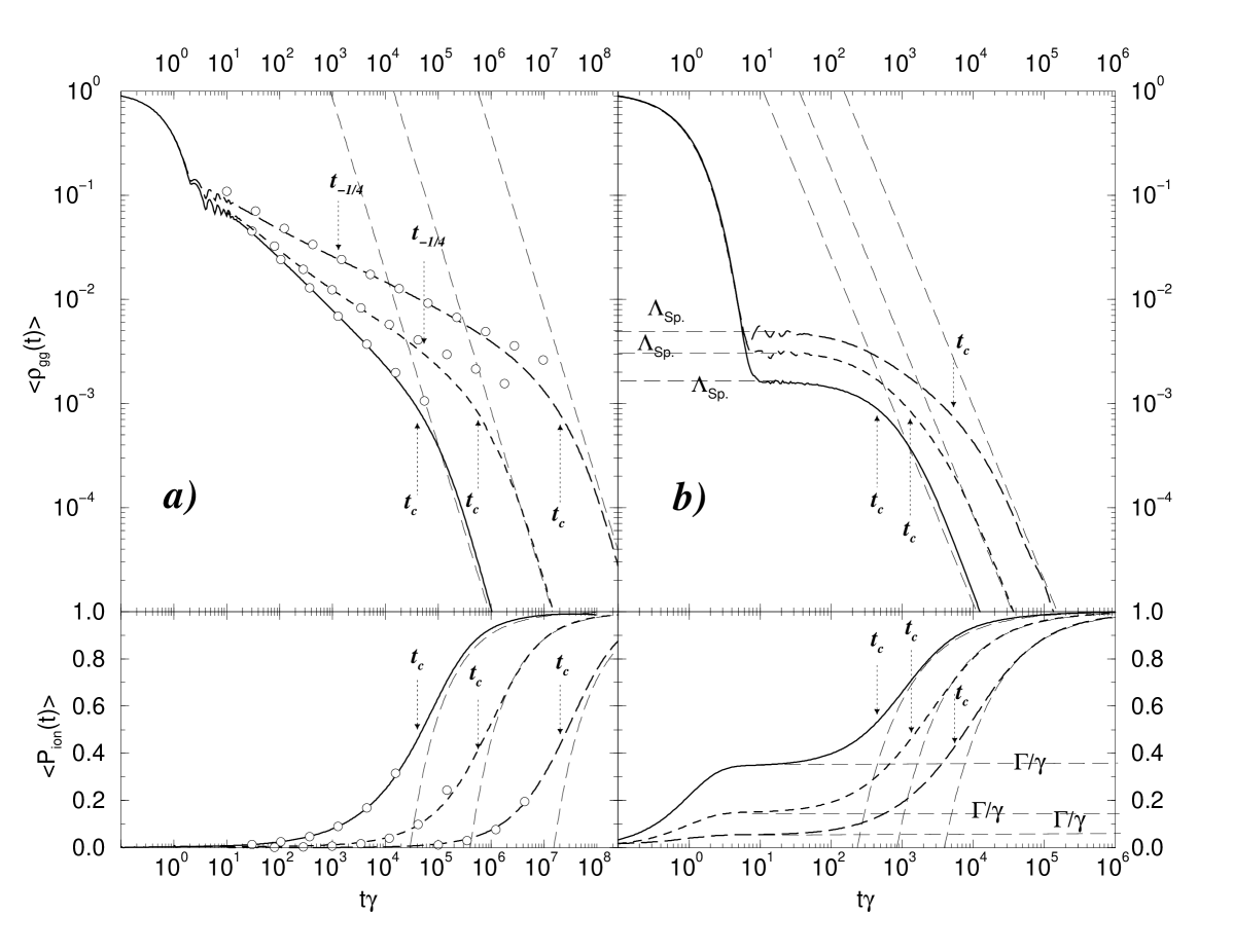
FIG. 3.: Mean initial state probability $\langle\rho_{gg}(t)\rangle$ and mean ionization probability $\langle P_{ion}(t)\rangle$ as a function of interaction time $t$ (in units of $1/\gamma$) for different values of $\beta$.
a) excitation well below threshold : $b/\gamma=5,T_{\overline{\epsilon}}\gamma=2,n_{res}=(-2\overline{\epsilon})^{-1/2}=200,\alpha=0.1$. PDM-limit $b/\beta=0$: (solid curve), $b/\beta=0.03$: (dashed curve), $b/\beta=0.2$: (long dashed curve), homogeneously spaced energy level limit according to Eqs.(50,51): (circles) and long time estimates according to Eqs.(37,38): (thin long dashed curves)
b) excitation at threshold : $b/\gamma=120,T_{\overline{\epsilon}}\gamma=10,\overline{\epsilon}/\gamma=-63.27,(-2\overline{\epsilon})^{-1/2}=200,\alpha=0.1$. PDM limit ($b/\beta=0$): (solid curve), strongly non-Lorentzian situations $b/\beta=3$: (dashed curve) and $b/\beta=10$: (long dashed curve). Long time estimates according to Eqs.(37,38): (thin long dashed curves).

In Fig.3b the laser bandwidth is so large that the significantly excited energy region $[\overline{\epsilon}-{\cal B},\overline{\epsilon}+{\cal B}]$ (before the onset of the electronic diffusion process) contains already the ionization threshold. Thus the excited Rydberg system is ionized significantly already in the early stages of the time evolution. As ${\cal B}\gg\gamma$ this early stage of the ionization process is well described by the DCA rate equations which yield (compare to Eqs.(45) and (46))

$$\langle\rho_{gg}(t)\rangle = e^{-\gamma t},$$ (83)

$$\langle P_{ion}(t)\rangle = \frac{\Gamma}{\gamma}(1-e^{-\gamma t}).$$ (84)

These approximate solutions are obtained from Eqs.(19) and (28) by neglecting $\langle\rho_{nn}(t)\rangle$ in comparison with $\langle\rho_{gg}(t)\rangle$. According to Eqs.(45) and (46) this initial ionization process saturates as soon as the mean initial state probability and the mean ionization probability have reached the values $\Lambda_{Sp}$ and $\Gamma/\gamma$. At these interaction times we still have $\gamma\Lambda_{Sp}t\ll 1$. These characteristic aspects of the laser-induced excitation process are clearly apparent in Fig.3b. Physically speaking in this initial stage of the excitation process the Rydberg electron is ionized with probability $\Gamma/\gamma$. With a probability of $(1-\Gamma/\gamma)$ an excited electronic Rydberg wave packet is prepared after a time of the order of $1/\gamma$. This wave packet is formed by a coherent superposition of all Rydberg states within the dominantly excited energy interval $[\overline{\epsilon}-{\cal B},0]$. Depending on the actual value of the laser bandwidth the coherent dynamics of this electronic wave packet is damped sooner or later. After the destruction of all coherences to a good degree of approximation the subsequent dynamics is governed by the DCA rate equations. In Fig. 3b small coherence oscillations are visible in the time evolution of $\langle\rho_{gg}(t)\rangle$. As soon as the interaction time exceeds the stochastic ionization time the excited Rydberg electron starts to ionize significantly. The time evolution of this stochastic ionization process is well described by Eqs.(37) and (38) within the framework of the DCA rate equations.

VII Summary and conclusion

The dynamics of an electronic Rydberg wave packet under the influence of a fluctuating cw-laser field has been discussed. It has been shown that for large laser bandwidths its dynamics can be described by Pauli-type rate equations for the relevant density matrix elements of the excited Rydberg electron averaged over the laser fluctuations. These rate equations are valid for arbitrary types of laser fluctuations and their dynamics is determined by the spectrum of the laser field only and not by any of the higher order correlation functions. The validity of these rate equations has been investigated in detail for a special class of phase fluctuations of the laser field.

With the help of these rate equations we have investigated the dynamics of a laser excited Rydberg electron for long interaction times. At these interaction times the dynamics of the Rydberg electron are dominated by stochastic diffusion in energy space towards the ionization threshold which leads finally to stochastic ionization. This diffusion process is accompanied by a characteristic scenario of power law decays. Analytical expressions have been derived for these power laws and their associated characteristic exponents. These analytical expressions exhibit in a clear way that the asymptotic power laws are independent of the quantum defect of the excited Rydberg states and to which extent they depend on details of the laser spectrum. In particular, it has been demonstrated that the characteristic exponents which describe the process of stochastic ionization are completely independent of the laser spectrum. However, the initial stages of the diffusion of the excited Rydberg electron depend on details of the laser spectrum.

Support by the Deutsche Forschungsgemeinschaft within the SPP ‘Zeitabhängige Phänomene und Methoden’ is acknowledged.

     

A Numerical solution technique for the Master equation

In this appendix an efficient numerical method for solving the master equation (77) is outlined.

First, we make a rearrangement of Eq.(77) splitting it into a PDM-part and an additional part that disappears in the limit $\beta\to\infty$, namely

$$\stackrel{{\scriptstyle\mbox{\boldmath$\cdot$}}}{{\rho}}(t)=-i\Bigl{[}H_{eff}\rho(t)-\rho(t)H^{\dagger}_{eff}\Bigr{]}+{\bf L}\rho(t).$$ (A1)

Thereby we have introduced the effective non-Hermitian Hamiltonian

$$H_{eff}=H_{dr.}-ib|g\rangle\!\langle g|,$$ (A2)

the damping operator

$${\bf L}\rho(t) = 2b|g\rangle\!\langle g|\rho(t)|g\rangle\!\langle g|$$ (A3)

$$+ b\int_{0}^{t}d\tau\sum_{n\not=g}\Bigl{\{}|n\rangle\!\langle n|\rho(t)|g\rangle\!\langle g|w_{n}(\tau)+\mbox{h.c.}\Bigr{\}}$$ (A4)

and a memory function

$$w_{n}=\lim_{\Omega\to\infty}\Omega e^{-\Omega\tau}-\alpha_{n}^{0}(\tau).$$ (A5)

In the PDM-limit, i.e. $\beta\to\infty$, the second term on the right side of Eq.(A3) disappears and the master equation reduces to Eq.(80). Integration of Eq.(A1) yields

$$\rho(t)=U(t)\rho(0)U^{\dagger}(t)+$$ (A6)

$$\qquad\qquad\ \ \int_{0}^{\infty}dt^{\prime}\Theta(t-t^{\prime})U(t-t^{\prime}){\bf L}\rho(t^{\prime})U^{\dagger}(t-t^{\prime})$$ (A7)

where $U(t)=\exp[-iH_{eff}t]$ is a non unitary time evolution operator. If the initial condition is taken to be $\rho(0)=|g\rangle\!\langle g|$, the Laplace transformed matrix elements of the density operator $\tilde{\rho}_{ij}(z)\equiv{\cal L}_{z}\rho_{ij}(t)\equiv\int_{0}^{\infty}\;dte^{izt}\rho_{ij}(t)$ become

$$\tilde{\rho}_{lk}(z)=H_{lggk}(z)\Bigl{[}1+2b\tilde{\rho}_{gg}(z)\Bigr{]}+$$ (A8)

$$b\sum_{n\not=g}\Bigl{\{}H_{lngk}(z)\tilde{w}_{n}(z)\tilde{\rho}_{ng}(z)+H_{lgnk}(z)\tilde{w}^{*}_{n}(-z)\tilde{\rho}_{gn}(z)\Bigr{\}},$$ (A9)

$$H_{abcd}(z)=$$ (A10)

$$\frac{1}{2\pi}\int_{-\infty}^{\infty}\!dz_{1}{\cal L}_{z_{1}+i0}\left\langle a\right|U(t)\left|b\right\rangle\left[{\cal L}_{z_{1}-z+i0}\left\langle d\right|U(t)\left|c\right\rangle\right]^{*}$$ (A11)

with $\tilde{w}_{n}(z)=1-\tilde{\alpha}_{n}^{0}(z)$. The Laplace transformed transition amplitudes ${\cal L}_{z}\left\langle i\right|U(t)\left|j\right\rangle$ appearing in Eq.(A10) are easily calculated [4, 6].

$${\cal L}_{z}\left\langle g\right|U(t)\left|g\right\rangle=\frac{i}{z+ib-\overline{\epsilon}-\Sigma(z)},$$ (A12)

$${\cal L}_{z}\left\langle g\right|U(t)\left|n\right\rangle={\cal L}_{z}\left\langle n\right|U(t)\left|g\right\rangle$$ (A13)

$$\qquad\qquad\qquad\ =\frac{-i\varepsilon_{0}d_{ng}}{(z-\epsilon_{n})[z+ib-\overline{\epsilon}-\Sigma(z)]},$$ (A14)

$${\cal L}_{z}\left\langle n\right|U(t)\left|l\right\rangle=$$ (A15)

$$\quad\quad\frac{1}{z-\epsilon_{n}}\Bigl{\{}i\delta_{nl}+\frac{i\varepsilon_{0}^{2}d_{ng}d_{lg}}{(z-\epsilon_{l})[z+ib-\overline{\epsilon}-\Sigma(z)]}\Bigr{\}}$$ (A16)

where $\Sigma(z)=\sum_{n\not=g}\frac{|\varepsilon_{0}d_{ng}|^{2}}{z-\epsilon_{n}}$ is the self energy of state $\left|g\right\rangle$ and the Kronecker-symbol $\delta_{nl}$ turns into a Dirac-delta function $\delta(\epsilon_{n}-\epsilon_{l})$ for energy normalized continuum states $\left|\epsilon_{n}\right\rangle$ and $\left|\epsilon_{l}\right\rangle$. For the subsequent treatment it is convenient to introduce the expressions

$$\alpha_{n}(z) = \frac{\tilde{\rho}_{ng}(z)}{[1+2b\tilde{\rho}_{gg}(z)]\varepsilon_{0}d_{ng}},$$ (A17)

$$\beta_{n}(z) = \frac{\tilde{\rho}_{gn}(z)}{[1+2b\tilde{\rho}_{gg}(z)]\varepsilon_{0}d_{ng}},$$ (A18)

$$E_{n}(z) = \frac{H_{gngg}(z)}{\varepsilon_{0}d_{ng}},\quad F_{n}(z)=\frac{H_{ggng}(z)}{\varepsilon_{0}d_{ng}}.$$ (A19)

Thus Eq.(A8) and Laplace transformation of Eq.(A1) yield

$$\tilde{\rho}_{gg}(z)=\frac{{\cal K}(z)}{1-2b{\cal K}(z)},$$ (A20)

$$\tilde{P}_{ion}(z)=$$ (A21)

$$\quad\frac{1}{2\pi(z+i0)(1-2b{\cal K}(z))}\int_{0}^{\infty}d\epsilon\bigl{[}\alpha_{\epsilon}(z)-\beta_{\epsilon}(z)\bigr{]}$$ (A22)

with the characteristic kernel

     

$${\cal K}(z)=H_{gggg}(z)+b\Bigl{(}\sum_{n\not=g}+\int_{0}^{\infty}dn(\epsilon)\Bigr{)}|\varepsilon_{0}d_{ng}|^{2}\Bigl{\{}E_{n}(z)\tilde{w}_{n}(z)\alpha_{n}(z)+F_{n}(z)\tilde{w}_{n}^{*}(-z)\beta_{n}(z)\Bigr{\}}$$ (A23)

and with

$$\alpha_{l}(z) = \frac{\tilde{w}_{l}^{*}(-z)C_{l}(z)|\varepsilon_{0}d_{lg}|^{2}\Bigl{(}F_{l}(z)+S_{l}(z)\Bigr{)}+\bigl{(}1-J_{l}(z)\bigr{)}\Bigl{(}E_{l}(z)+T_{l}(z)\Bigr{)}}{\bigl{(}1-G_{l}(z)\bigr{)}\bigl{(}1-J_{l}(z)\bigr{)}-(\tilde{w}_{l}(z)\tilde{w}_{l}^{*}(-z))^{2}C_{l}(z)^{2}|d_{lg}|^{4}},$$ (A24)

$$\beta_{l}(z) = \frac{w_{l}(z)C_{l}(z)|\varepsilon_{0}d_{lg}|^{2}\Bigl{(}E_{l}(z)+T_{l}(z)\Bigr{)}+\bigl{(}1-G_{l}(z)\bigr{)}\Bigl{(}F_{l}(z)+S_{l}(z)\Bigr{)}}{\bigl{(}1-G_{l}(z)\bigr{)}\bigl{(}1-J_{l}(z)\bigr{)}-(\tilde{w}_{l}(z)\tilde{w}_{l}^{*}(-z))^{2}C_{l}(z)^{2}|d_{lg}|^{4}}.$$ (A25)

The non-diagonal couplings $(\alpha_{l},\beta_{l}\leftrightarrow\alpha_{n},\beta_{n},\quad n\not=l)$ due to the sum in Eq.(A8) give rise to the expressions $S_{l}(z)$ and $T_{l}(z)$ appearing in Eqs.(A24) and (A25), namely

$$S_{l}(z) = b\Bigl{\{}\sum_{n\not=\{g,l\}}+\int_{0}^{\infty}dn(\epsilon)\Bigr{\}}|\varepsilon_{0}d_{ng}|^{2}\Bigl{[}\beta_{n}(z)\frac{F_{n}(z)-F_{l}(z)}{\epsilon_{l}-\epsilon_{n}}-\alpha_{n}(z)\frac{F_{l}(z)-E_{n}(z)}{\epsilon_{n}-\epsilon_{l}-z-2i0}\Bigr{]},$$ (A26)

$$T_{l}(z) = b\Bigl{\{}\sum_{n\not=\{g,l\}}+\int_{0}^{\infty}dn(\epsilon)\Bigr{\}}|\varepsilon_{0}d_{ng}|^{2}\Bigl{[}\alpha_{n}(z)\frac{E_{n}(z)-E_{l}(z)}{\epsilon_{l}-\epsilon_{n}}-\beta_{n}(z)\frac{E_{l}(z)-F_{n}(z)}{\epsilon_{n}-\epsilon_{l}+z+2i0}\Bigr{]}.$$ (A27)

The diagonal couplings of the $\alpha_{n}$ and $\beta_{n}$ yield $J_{l}(z),G_{l}(z)$ and $C_{l}(z)$, i.e.

$$C_{l}(z) = b\Theta(-\epsilon_{l})\frac{E_{l}(z)-F_{l}(z)}{z+2i0},$$ (A28)

$$G_{l}(z) = \frac{b\tilde{w}_{l}(z)}{2\pi}\int_{-\infty}^{\infty}\frac{dz_{1}\Bigl{\{}1+\Theta(-\epsilon_{l})|\varepsilon_{0}d_{lg}|^{2}\bigl{[}z_{1}+ib-\overline{\epsilon}-\Sigma(z_{1}+i0)\bigr{]}^{-1}(z_{1}-\epsilon_{l}+i0)^{-1}\Bigr{\}}}{\bigl{[}z_{1}-z-ib-\overline{\epsilon}-\Sigma(z_{1}-z-i0)\bigr{]}(z_{1}-\epsilon_{l}+i0)},$$ (A29)

$$J_{l}(z) = \frac{b\tilde{w}_{l}^{*}(-z)}{2\pi}\int_{-\infty}^{\infty}\frac{dz_{1}\Bigl{\{}1+\Theta(-\epsilon_{l})|\varepsilon_{0}d_{lg}|^{2}\bigl{[}z_{1}-z-ib-\overline{\epsilon}-\Sigma(z_{1}-z-i0)\bigr{]}^{-1}(z_{1}-z-\epsilon_{l}-i0)^{-1}\Bigr{\}}}{\bigl{[}z_{1}+ib-\overline{\epsilon}-\Sigma(z_{1}+i0)\bigr{]}(z_{1}-z-\epsilon_{l}-i0)}.$$ (A30)

All information about the quantum system is contained in the self energy $\Sigma(z)$. In order to solve Eqs.(A24-A27) for a given value of $z$, the coefficients $H_{gggg},E_{l},F_{l},J_{l}$ and $G_{l}$ have to be calculated. Using the energy levels and dipole matrix elements of Eqs.(12) the self energy becomes [4]

$$\Sigma(z) = \delta\omega-i\frac{\gamma}{2}+i\gamma\frac{1}{1-\exp(-2\pi i\nu(z))]}$$ (A31)

$$\mbox{with}\qquad\nu(z) = (-2z)^{-1/2}+\alpha$$ (A32)

and with the (non-resonant) quadratic Stark-shift contribution $\delta\omega$. In[6] we calculated the quantity $H_{gggg}$ ($f(z)$ in that work) by contour integration. In an analogous way the quantities $E_{l},F_{l},J_{l}$ and $G_{l}$ can be calculated but for sake of brevity we do not give them here explicitly. Starting with $S_{n}=T_{n}=0$, Eqs.(A20-A27) are solved by iteration. Actually we found the non-diagonal coupling terms $S_{l},T_{l}$ to be very small in comparison with the diagonal couplings so that this iteration converges very rapidly.

REFERENCES

• [1] M.J.Seaton, Rep. Prog. Phys. 46, 167 (1983)
• [2] M.Aymar, Ch.H.Greene and E.Luc-Koenig, Rev.Mod.Phys.68, 1015 (1996)
• [3] A.R.P.Rau and M.Inokuti, Am.J.Phys. 65, 221 (1997)
• [4] G.Alber and P.Zoller, Phys.Rev.A 37, 377 (1988)
• [5] A.Giusti-Suzor and P.Zoller, Phys.Rev.A 36, 5178 (1987)
• [6] G.Alber and B.Eggers, Phys.Rev.A 56, 820 (1997)
• [7] H.Haken in Handbuch der Physik edited by S.FlΓΌgge (Springer, New York 1970),Vol. XXV/2c
• [8] M.O.Scully and M.S.Zubairy, Quantum Optics (Cambridge, Cambridge, 1997)
• [9] S.N.Β Dixit, P.Β Zoller, and P.Β Lambropoulos, Phys.Β Rev.Β AΒ 21, 1289 (1980)
• [10] D.S.Elliot, M.W.Hamilton, K.Arnett und S.J.Smith, Phys.Rev.A 32 887 (1985)
• [11] P.E.Kloeden and E.Platen, Numerical Solution of Stochastic Differential Equations (Springer, Berlin 1992)
• [12] S.G.Agarval Phys.Rev.Lett. 37, 1383 (1976); Phys.Rev.A 18, 1490 (1978)
• [13] M.Abramowitz and I.Stegun, Handbook of Mathematical Functions (Dover Publications, N.Y. 1972)