Absorption-free discrimination between Semi-Transparent Objects

Abstract

Absorption-free (also known as “interaction-free”) measurement aims to detect the presence of an opaque object using a test particle without that particle being absorbed by the object. Here we consider semi-transparent objects which have an amplitude $\alpha$ of transmitting a particle while leaving the state of the object unchanged and an amplitude $\beta$ of absorbing the particle. The task is to devise a protocol that can decide which of two known transmission amplitudes is present while ensuring that no particle interacts with the object. We show that the probabilities of being able to achieve this are limited by an inequality. This inequality implies that absorption free distinction between complete transparency and any partial transparency is always possible with probabilities approaching 1, but that two partial transparencies can only be distinguished with probabilities less than 1.

PACS numbers: 03.65.Bz, 03.67.-a

In “interaction-free” measurement the task is to decide, using a test particle, whether an opaque object is present or absent while ensuring that the test particle is not absorbed by the object. Many methods for achieving this have been devised [1, 2, 3, 4, 5, 6, 7]. The essential idea behind all of them is that the measurement picks a set of histories in none of which an interaction between object and test particle takes place, so no absorption occurs; other histories in the protocol will involve interactions, and in this sense the term “absorption-free” may be preferred to the more commonly-used term “interaction-free”. We abbreviate absorption-free measurement to AFM henceforth.

In standard AFM, the object is considered to be either completely opaque or completely transparent (absent). One can also consider semi-transparent objects, for which there is an amplitude $\alpha$ of the particle passing through the object while leaving the state of the object unchanged and an amplitude $\beta$ for the particle to interact with the object and hence be absorbed, leaving the object in an “interacted” state (in Elitzur and Vaidman’s proposal this is the exploded state of the bomb). One can then ask whether one can infer the transmission amplitude of the object while ensuring that the object never reaches the “interacted” state. This is the problem we consider here, in the case where there are two known transmission amplitudes that have to be distinguished.

This problem is of obvious practical interest. Indeed there are situations where one wants to determine the nature of an object but where radiation will damage the object, for instance when imaging a biological specimen in the ultraviolet. In these cases one wants to minimize the amount of radiation absorbed by the object. Standard AFM shows that if the object has only two possible states, completely transparent or completely opaque, then it is possible to determine the state without any photon being absorbed. However most objects will be semi-transparent. Here we address this more general case.

In [8], a general framework for counterfactual quantum events was proposed, which includes AFM. Two variables $\left|p\right\rangle$ and $\left|q\right\rangle$ are distinguished in the total state space. The first variable $\left|p\right\rangle$ defines the state of the particle and its position within the apparatus used for AFM, and we assume there is a particular subset of values, $\cal I$, for which interactions between the particle and apparatus can occur leading to absorption. The second variable $\left|q\right\rangle$, which we call the interaction variable, takes the value $\left|1\right\rangle$ if absorption occurs and $\left|0\right\rangle$ if not. It may have additional values, but they play no role in the following discussion.

Any protocol for AFM can be divided into a series of steps. In some of these steps an interaction can potentially occur; we call these I-steps. An I-step has two parts. The first is a unitary transformation given by

$$\begin{array}[]{ll}\left|p0\right\rangle\rightarrow\alpha\left|p0\right\rangle+\beta\left|p1\right\rangle&p\in\cal I\\ \left|p0\right\rangle\rightarrow\left|p0\right\rangle&p\notin\cal I\end{array}$$ (1)

where $\alpha$, $\beta$ are complex numbers satisfying $|\alpha|^{2}+|\beta|^{2}=1$. The second part is a measurement of the interaction variable in the basis $\left|0\right\rangle$, $\left|1\right\rangle$. The unitary transformation is not fully defined by (1), but we do not need to specify its action on terms like $\left|p1\right\rangle$ since we are concerned with histories on which no interaction occurs, and a protocol can be assumed to halt when measurement of the interaction variable yields $\left|1\right\rangle$.

A protocol for AFM starts from a specified initial state. It is allowed to undergo a unitary transformation between successive I-steps, this transformation leaving the interaction variable unchanged. At the end of the protocol the variable $\left|p\right\rangle$ is measured. A protocol with measurements of $\left|p\right\rangle$ before the end can be converted to the form we specify by entangling the measured variables with extra variables and postponing their measurement till the end [8].

In all the protocols, there are two measurement outcomes, $M_{1}$ and $M_{2}$ say, the first of which indicates that the object was absent, while the second indicates that the object was present and also that no absorption occurred. There will also be other outcomes, for instance that an absorption occurred. We denote the probability of $M_{i}$ by $P(ident|i)$, i.e. the probability of identifying, without the particle being absorbed, whether the object is present ($i=2$) or absent ($i=1$). The probabilities $P(ident|i)$ give an indication of the efficiency of the protocol. In Elitzur and Vaidman’s original proposal [3], one has $P(ident|2)=1/4$ and $P(ident|1)=0$. In many recent protocols, $P(ident|2)=1$ and $P(ident|1)$ tends to 1.

Figure 1 shows two types of AFM protocol. The quantum Zeno type [4, 5] is an elaboration of Elitzur and Vaidman’s original proposal [3]. We have adapted it so that it can distinguish between no object ($\alpha_{1}=1$) and an object of transmission amplitude $0\leq|\alpha_{2}|<1$. We take the first qubit of $|pq\rangle$ to correspond to polarization, and the initial state is a vertically polarized photon, denoted $|v0\rangle$. The AFM consists of repeated passages through a polarization rotator, a Mach-Zender interferometer, and a second polarization rotator. After the first rotation the state becomes $\cos\theta|v0\rangle+\sin\theta|h0\rangle$. After passing through the polarization beam splitter, the horizontally polarised component $\left|h0\right\rangle$ goes along the lower path, that may contain the object, whereas $\left|v0\right\rangle$ takes the object-free upward-going path. In this case, therefore, $\cal I$ is the single value $p=h$. Applying (1), the I-step gives the un-normalised state $\left|\psi_{i}\right\rangle=\cos\theta\left|v0\right\rangle+\alpha_{i}\sin\theta\left|h0\right\rangle$. The second polarization beam splitter then recombines the two polarizations into one beam. If $\alpha_{2}$ is real and positive, then the state in case $i=2$ can be rewritten as $\left|\psi_{2}\right\rangle=\gamma\left(\cos\theta^{\prime}\left|v0\right\rangle+\sin\theta^{\prime}\left|h0\right\rangle\right)$ where $\cos\theta^{\prime}=\cos\theta/\sqrt{\cos^{2}\theta+\alpha_{2}^{2}\sin^{2}\theta}$ (note that $\theta^{\prime}\leq\theta$). The final step is a rotation by the angle $-\theta^{\prime}$. This brings the state to $\cos(\theta-\theta^{\prime})|v0\rangle+\sin(\theta-\theta^{\prime})\left|h0\right\rangle$ (no object present) or $\gamma|v0\rangle$ (object present). We then iterate this procedure $N$ times, choosing $N$ such that $N(\theta-\theta^{\prime})=\pi/2$. This brings the state to $|h0\rangle$ (no object present) or $\gamma^{N}|v0\rangle$ (object present). Since these states are orthogonal $P(ident|1)=1$ and $P(ident|2)=\gamma^{2N}$. For large $N$ (small $\theta$), $\gamma\simeq 1-{(1+\alpha_{2})\pi^{2}\over(1-\alpha_{2})4N^{2}}$ and $P(ident|2)\to 1$.

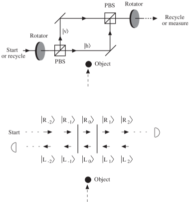
FIG. 1.: Two absorption-free measurement protocols. In the quantum Zeno type (above) the photon is passed through a rotator, followed by two polarising beam-splitters (PBS) and a final polarisation rotator, and is then recycled a certain number of times. In our protocol for $\alpha_{1}=1$, $\alpha_{2}$ real, the first rotation is by an angle $\theta$ and the second is by an angle $(\theta-\theta^{\prime})$ (see text). In the Fabry-Perot type (below), the plane wave representing the photon is decomposed into a superposition of wave packets. The wave function for a right-going pulse at position $i$ is denoted by $\left|R_{i}\right\rangle$ and for a left-going pulse by $\left|L_{i}\right\rangle$. If an object is inserted in the cavity (between the two vertical lines) the photon may be reflected to the left. If there is no object, it will be transmitted to the right.

If $\alpha_{2}=|\alpha_{2}|e^{i\phi_{2}}$ has a non zero phase (the phase is defined by the convention that $\alpha_{1}=1$) then after recombining the two beams the state is $\left|\psi_{2}\right\rangle=\gamma\left(\cos\theta^{\prime}\left|v0\right\rangle+\sin\theta^{\prime}e^{i\phi_{2}}\left|h0\right\rangle\right)$. The final rotation is chosen so as to take this state to the state $\gamma|v0\rangle$ and to take the state if no object is present to $\cos\omega|v0\rangle+\sin\omega|h0\rangle$ where $\theta-\theta^{\prime}\leq\omega\leq\theta+\theta^{\prime}$. Iterating this procedure $N$ times, with $N\omega=\pi/2$, and then carrying out a measurement of polarisation, realizes an AFM.

An alternative type of AFM protocol uses the concept of a monolithic total-internal-reflection resonator [6], or a Fabry-Perot (F-P) interferometer [7]. In the case of the F-P there is a photon of momentum $k$ incoming from the left, and one measures whether the photon is reflected or transmitted. To see how the F-P fits into our framework for AFM, we make the dynamics discrete to correspond to the steps in a protocol. Define a lattice of spacing $d$ (the spacing of the mirrors, see Figure 1(b)) and let each step in the protocol correspond to a time $t=d/c$. The state $|R_{n}\rangle$ corresponds to a segment of right-moving plane wave over the spatial range $[nd,(n+1)d]$ for time interval $t$, and $|L_{n}\rangle$ to the corresponding segment of left-moving plane wave. Over time $t$, $|R_{n}\rangle$ evolves into $|R_{n+1}\rangle$ and $|L_{n}\rangle$ into $|L_{n-1}\rangle$, except in the vicinity of the mirrors, where we have $\left|R_{0}\right\rangle\rightarrow c\left|L_{0}\right\rangle+is\left|R_{1}\right\rangle$, $\left|R_{-1}\right\rangle\rightarrow c\left|L_{-1}\right\rangle+is\left|R_{0}\right\rangle$, $\left|L_{1}\right\rangle\rightarrow c\left|R_{1}\right\rangle+is\left|L_{0}\right\rangle$, and $\left|L_{0}\right\rangle\rightarrow c\left|R_{0}\right\rangle+is\left|L_{-1}\right\rangle$, $c$ and $is$ being reflection and transmission coefficients, respectively.

We have treated the mirrors as dispersionless, which is a mathematical convenience to restrict ourselves to the Fourier component of the incoming plane wave. We have also taken $d$ such that $e^{idk}=1$ (where $k$ is the wave number of the plane wave) so that no phase is accumulated between the mirrors.

If an object of transparency $\alpha$ is inserted between the two mirrors, the discretised dynamics, conditional on no photon being absorbed, becomes $\left|R_{0}\right\rangle\rightarrow\alpha\left(c\left|L_{0}\right\rangle+is\left|R_{1}\right\rangle\right)$, $\left|R_{-1}\right\rangle\rightarrow c\left|L_{-1}\right\rangle+is\left|R_{0}\right\rangle$, $\left|L_{1}\right\rangle\rightarrow c\left|R_{1}\right\rangle+is\left|L_{0}\right\rangle$, and $\left|L_{0}\right\rangle\rightarrow\alpha\left(c\left|R_{0}\right\rangle+is\left|L_{-1}\right\rangle\right)$. Thus ${\cal I}=\{L_{0},R_{0}\}$, since interaction can only occur within the apparatus.

The initial state is $e^{ikx}=\sum^{n=-1}_{-\infty}\left|R_{n}\right\rangle$. After many time steps, one settles into a steady state regime and the state outgoing to the left $f_{L}$ is the sum of the pulses reflected once by the left mirror and those reflected $2m-1$ times inside the instrument and traversing the object $2m$ times, for $m=1,2,\ldots$:

$$f_{L} = \sum^{n=-1}_{-\infty}\left|L_{n}\right\rangle\left(c+s^{2}\sum^{\infty}_{m=1}c^{2m-1}\alpha^{2m}\right)$$

$$= \sum^{n=-1}_{-\infty}\left|L_{n}\right\rangle\frac{c(1-\alpha^{2})}{1-c^{2}\alpha^{2}}.$$

As $c\to 1$, the probability $|f_{L}|^{2}=|c(1-\alpha^{2})/(1-c^{2}\alpha^{2})|^{2}$ of reflection to the left tends to 1, except when $\alpha=1$ (object absent) in which case the probability of transmission to the right is 1. Thus the F-P allows an absorption-free discrimination between the absence of an object ($\alpha_{1}=1$) and the presence of an object of transparency $\alpha_{2}\neq 1$.

Now consider any protocol that falls within our general scheme, and suppose that one must distinguish between two semi-transparent objects with transmission amplitude $\alpha_{1}$, $\alpha_{2}$ (which can both be different from $1$) and interaction amplitude $\beta_{1}$, $\beta_{2}$ respectively. We shall prove the following constraint on the probability $P(ident|i)$ of identifying transparency $\alpha_{i}$ without any absorption occurring:

Theorem: $(1-P(ident|1))(1-P(ident|2))\geq\eta^{2}$, where $\eta=|\beta_{1}\beta_{2}/(1-\bar{\alpha}_{1}\alpha_{2})|$.

Before giving the proof, we look at some of the consequences of this inequality. First, note that $|1-\bar{\alpha}_{1}\alpha_{2}|^{2}-|\beta_{1}\beta_{2}|^{2}=|\alpha_{1}-\alpha_{2}|^{2}$. Thus $\eta\leq 1$, and $\eta=1$ iff $\alpha_{1}=\alpha_{2}$. This implies that $P(ident|1)=P(ident|2)=0$ when $\alpha_{1}=\alpha_{2}$, which must of course be the case, since two equal transmission amplitudes cannot be distinguished. Whenever $\alpha_{1}\neq\alpha_{2}$, however, the theorem allows non-zero values of $P(ident|1)$ and $P(ident|2)$.

Another special case is when one object is completely transparent (absent), ie. $|\alpha_{1}|=1$ and $\beta_{1}=0$. If $\alpha_{2}\neq\alpha_{1}$, then $\eta=0$, and the theorem permits $P(ident|1)=P(ident|2)=1$. That this can be achieved was shown above.

The most significant aspect of this result is that when both $|\alpha_{1}|$ and $|\alpha_{2}|$ are different from $1$, that is neither object is completely transparent, then $\eta$ is strictly positive. This implies that both $P(ident|1)$ and $P(ident|2)$ must be strictly less than $1$. Thus it is impossible to identify two semi-transparent objects with vanishing probability that the test particle is absorbed by the objects. This is bad news for the applications outlined above.

Proof: The total state space can be decomposed into two orthogonal subspaces, the first spanned by components whose first variable $p$ satisfies $p\notin\cal I$, and the second by components whose first variable $p$ satisfies $p\in\cal I$. Recall that a general protocol can be written as a series of I-steps followed by unitary transformations. We can write the un-normalized state for transparency $i$ at stage $k$ of the protocol immediately before the I-step as $\left|u_{i}^{k}\right\rangle+\left|v_{i}^{k}\right\rangle$, where $\left|u_{i}^{k}\right\rangle$ lies in the first subspace and $\left|v_{i}^{k}\right\rangle$ in the second. Immediately after the I-step (1) implies that the un-normalized state is

$\displaystyle\left|\psi_{i}^{k}\right\rangle=\left|u_{i}^{k}\right\rangle+\alpha_{i}\left|v_{i}^{k}\right\rangle.$

We assume that the states $\left|\psi_{i}^{k}\right\rangle$ are all un-normalized, so $1-|\psi_{i}^{k}|^{2}$ is the probability of no absorption occurring up to stage $k$ of the protocol. After the I-step there is a unitary transformation that carries $\left|\psi_{i}^{k}\right\rangle$ to $\left|u_{i}^{k+1}\right\rangle+\left|v_{i}^{k+1}\right\rangle$. We define

$$f^{k}=\langle\psi_{1}^{k}|\psi_{2}^{k}\rangle,$$ (2)

whereupon unitarity implies

$$f^{k} = \langle u_{1}^{k+1}+v_{1}^{k+1}|u_{2}^{k+1}+v_{2}^{k+1}\rangle$$

$$= \langle u_{1}^{k+1}|u_{2}^{k+1}\rangle+\langle v_{1}^{k+1}|v_{2}^{k+1}\rangle$$

(since the components $u$ and $v$ lie in orthogonal subspaces), and (2) for $k+1$ implies

$\displaystyle f^{k+1}=\langle u_{1}^{k+1}|u_{2}^{k+1}\rangle+\bar{\alpha}_{1}\alpha_{2}\langle v_{1}^{k+1}|v_{2}^{k+1}\rangle.$

We therefore get

$\displaystyle f^{k+1}=f^{k}-(1-\bar{\alpha}_{1}\alpha_{2})\langle v_{1}^{k+1}|v_{2}^{k+1}\rangle,$

and hence

$\displaystyle f^{N}=1-(1-\bar{\alpha}_{1}\alpha_{2})\sum_{k=0}^{N-1}\langle v_{1}^{k+1}|v_{2}^{k+1}\rangle,$

where the $N$-th step is the last step of the protocol before the final measurement. This implies

$\displaystyle{|1-f^{N}|^{2}\over|1-\bar{\alpha}_{1}\alpha_{2}|^{2}}=|\sum_{k=0}^{N-1}\langle v_{1}^{k+1}|v_{2}^{k+1}\rangle|^{2}\ .$

We now use the Cauchy-Schwartz inequality to obtain

$${|1-f^{N}|^{2}\over|1-\bar{\alpha}_{1}\alpha_{2}|^{2}}\leq\sum_{k=0}^{N-1}|v_{1}^{k+1}|^{2}\sum_{k=0}^{N-1}|v_{2}^{k+1}|^{2}\ .$$ (3)

The probability that an interaction occurs during the k’th I-step is $|\beta_{i}|^{2}|v^{k}_{i}|^{2}$, and therefore we can rewrite (3) as

$${|1-f^{N}|^{2}|\beta_{1}|^{2}|\beta_{2}|^{2}\over|1-\bar{\alpha}_{1}\alpha_{2}|^{2}}\leq P(interact|1)P(interact|2)$$ (4)

where $P(interact|i)=|\beta_{i}|^{2}\sum|v_{i}^{k+1}|^{2}$ is the total probability of interaction for transparency $i$.

We now turn to the final measurement. There are three possible outcomes. The first is that the test particle is absorbed by the object. The second is that the particle is not absorbed and that the object is identified. The third is that no absorption occurs but the object is not identified. This occurs with probability $P(NOTident|i)$. Our aim is to construct a measurement setup such that $P(ident|i)$ is as large as possible. To this end we note that an optimal setup necessarily has $P(NOTident|i)=0$. Indeed suppose that $P(NOTident|i)\neq 0$. Then we run the protocol once, and if we obtain the outcome $NOTident$ we run the protocol a second time (constructing a protocol with its measurement of $\left|p\right\rangle$ at the end by entangling the outcomes of the first protocol with extra qubits). This increases the probability of identifying the object from $P(ident|i)$ to $P(ident|i)(1+P(NOTident|i))$. This procedure can be iterated many times to ensure that the probability of not identifying the object is as small as we wish.

Upon taking the limit $P(NOTident|i)\to 0$ one finds that $P(interact|i)\to 1-P(ident|i)$ and that $f^{N}\to 0$. The latter limit is because if the two states $\psi^{N}_{i}$ can be identified with certainty, their scalar product must be zero. Thus in the limit $P(NOTident|i)\to 0$, (4) tends to the inequality of the theorem. If $P(NOTident|i)\neq 0$, then $P(ident|i)$ is necessarily smaller than in the limiting case, and the inequality is also obeyed. $\Box$

This result establishes some limits on AFM of semi-transparent objects. It also raises various questions. First, can the bound be attained? We showed above that this is the case if one of the objects is transparent. The following numerical procedure suggests that the bound can be approached very closely for any real $\alpha_{i}$.

Consider a quantum Zeno protocol based on a polarisation degree of freedom as described above. We denote by $\left|\psi^{k}_{i}\right\rangle=\left|v0\right\rangle a^{k}_{i}+\left|h0\right\rangle b^{k}_{i}$ the state for transparency $i$ at stage $k$. Suppose $\left|\psi^{k+1}_{i}\right\rangle$ is obtained from $\left|\psi^{k}_{i}\right\rangle$ by a rotation of angle $\theta^{k}$ followed by an I-step. Then we have $a^{k+1}_{i}=\cos\theta^{k}a^{k}_{i}-\sin\theta^{k}b^{k}_{i}$ and $b^{k+1}_{i}=\alpha_{i}(\sin\theta^{k}a^{k}_{i}+\cos\theta^{k}b^{k}_{i})$, for $i=1,2$. Pick $\lambda$ and require $b^{k}_{2}/b^{k}_{1}=\lambda$ for all $k$, this being the condition for equality in the Cauchy-Schwartz step leading to equation (3). This would imply

$\displaystyle\tan\theta^{k}=\frac{\alpha_{1}b^{k}_{1}\lambda-\alpha_{2}b^{k}_{2}}{\alpha_{2}a^{k}_{2}-\alpha_{1}a^{k}_{1}\lambda},$

which can be used to generate a series of angles $\theta^{k}$. However, there is a problem with starting the procedure, since the initial state must be the same for $i=1,2$, and so the ratio $b^{0}_{2}/b^{0}_{1}$ must be 1. Yet we wish to choose $\lambda$ freely. By taking $b^{0}_{i}=\epsilon$, $a^{0}_{i}=\sqrt{1-\epsilon^{2}}$, $i=1,2$, for small $\epsilon$, we ensure that the initial terms $b^{0}_{i}$ are small and thereafter for larger terms $b^{k}_{i}$ the ratio $b^{k}_{2}/b^{k}_{1}$ is $\lambda$. This means that the condition for equality in Cauchy-Schwartz comes very close to being satisfied.

Simulations show that a simple search always comes up with a value of $\lambda$ that makes the $\left|\psi^{N}_{i}\right\rangle$’s very close to orthogonal after some number of steps $N$. One can therefore make a final measurement at the $N$-th step using a POVM, in which the components yielding the AFM outcomes $M_{1}$ and $M_{2}$ are very close to the $\left|\psi^{N}_{i}\right\rangle$’s. By taking $\epsilon$ small enough one can make the approach to equality of $(1-P(ident|1))(1-P(ident|2))$ and $\eta^{2}$ as near as one likes for any $\alpha$’s (eg see Figure 2). It would be interesting to prove analytically that this must be so, and also to extend it to complex amplitudes.

FIG. 2.: Sequences of angles $\theta^{k}$ (omitting a long run-in and tail of very small angles) derived from the procedure for making near-optimal quantum Zeno protocols, with $\alpha_{1}=0.8$, $\alpha_{2}=0.82$. The value of $(1-P(ident|1))(1-P(ident|2))=0.996621$ given by the algorithm is very close to $\eta^{2}=0.996620$. Here $\epsilon$ was taken to be $0.0001$ and the value of $\lambda$ generated by the numerical search was 1.049996.

A second question concerns interaction-free discrimination of more than two transparencies. What bounds apply in this case? We can also broaden the question and consider situations where the object is not destroyed when one particle interacts with it (eg the Elitzur-Vaidman bomb), but where one wants to minimize the amount of interaction (eg to reduce potential radiation damage). What bounds apply to minimal absorption measurements [9]?

We thank Richard Jozsa, Noah Linden, Sandu Popescu and Stefano Pironio for helpful discussion. Particular thanks to Sandu Popescu for raising the question of whether two grey levels can be distinguished by an AFM. S.M. is a research associate of the Belgian National Research Fund. He thanks the European Science Foundation for financial support.

REFERENCES

- [1] Renninger, M. Z. Phys. 158, 417-420 (1960).
- [2] Dicke, R. H., Am. J. Phys. 49, 925-930 (1981).
- [3] Elitzur, A. C. and Vaidman, L., Found. Phys. 23, 987-997 (1993).
- [4] Kwiat, P. G., Weinfurter, H., Herzog, T., Zeilinger, A. and Kasevich, M. A., Phys. Rev. Lett. 74, 4763-4766 (1995).
- [5] Kwiat, P. G., White, A. G., Mitchell, J. R., Nairz, O., Weihs, G., Weinfurter, H. and Zeilinger, A., preprint available at http://xxx.lanl.gov/quant-ph/9909083 (1999).
- [6] Paul, H. and Pavicic, M., J. Opt. Soc. America B 14, 1273-1277 (1997).
- [7] Tsegaye, T., Goobar, A., Karlsson, A., Bjork, G., Loh, M. Y. and Lim, K. H., Phys. Rev. A 57, 3987-3990 (1998).
- [8] Mitchison, G. and Jozsa, R., preprint available at http://xxx.lanl.gov/quant-ph/9907007 (1999).
- [9] Krenn, G., Summhammer, J., Svozil, K., Phys. Rev. A 61, 052102-1 to 10 (2000).