Spontaneous decay in the presence of dispersing and absorbing bodies:
general theory and application to a spherical cavity

Abstract

A formalism for studying spontaneous decay of an excited two-level atom in the presence of dispersing and absorbing dielectric bodies is developed. An integral equation, which is suitable for numerical solution, is derived for the atomic upper-state-probability amplitude. The emission pattern and the power spectrum of the emitted light are expressed in terms of the Green tensor of the dielectric-matter formation including absorption and dispersion. The theory is applied to the spontaneous decay of an excited atom at the center of a three-layered spherical cavity, with the cavity wall being modeled by a band-gap dielectric of Lorentz type. Both weak coupling and strong coupling are studied, the latter with special emphasis on the cases where the atomic transition is (i) in the normal-dispersion zone near the medium resonance and (ii) in the anomalous-dispersion zone associated with the band gap. In a single-resonance approximation, conditions of the appearance of Rabi oscillations and closed solutions to the evolution of the atomic state population are derived, which are in good agreement with the exact numerical results.

I Introduction

It is well known that the spontaneous decay of an excited atom can be strongly modified when it is placed inside a microcavity [2, 3]. There are typically two qualitatively different regimes: the weak-coupling regime and the strong-coupling regime. The weak-coupling regime is characterized by monotonous exponential decay, the decay rate being enhanced or reduced compared to the free-space value depending on whether the atomic transition frequency fits a cavity resonance or not. The strong-coupling regime, in contrast, is characterized by reversible Rabi oscillations where the energy of the initially atom is periodically exchanged between the atom and the field. This usually requires that the emission is in resonance with a high-quality cavity mode. Recent progress in constructing certain types of microcavities such as microspheres has rendered it possible to approach the ultimate quality level determined by intrinsic material losses [4], so that the question of the influence of absorbing material on spontaneous decay has been of increasing interest.

Effects of material losses on the lifetime of an excited atom have been studied within Fermi’s golden-rule approach [5, 6, 7, 8, 9, 10, 11, 12]. In [13] the mode structure of a microsphere without and with absorber dopant atoms, which is modeled by a constant and a Lorentzian dielectric function respectively, is considered. The spontaneous emission rate and the radiation intensity as a function of the atomic transition frequency is examined in [14] for an atom in a Fabry-Perot cavity filled with a Lorentz-type dielectric in the case of strong medium-cavity interaction but weak atom-field interaction.

In this paper we present a theory of the spontaneous decay of an excited two-level atom in the presence of arbitrary dispersing and absorbing dielectric bodies. We apply the theory to the spontaneous decay of an atom in a spherical microcavity of given complex-valued refractive-index profile, as it is typically the case in experimental implementations. The formalism enables us to include in the theory absorption and dispersion in a consistent way and to give a unified treatment of spontaneous emission, without restriction to a particular coupling regime.

The plan of the paper is as follows. In Section II, a recently developed quantization scheme for the electromagnetic field in the presence of dispersing and absorbing dielectric bodies [15, 16, 17, 18] is extended in order to include in the theory the resonant interaction of the field with a two-level atom. From the Hamiltonian of the composed system, an integral equation governing the temporal evolution of the upper-level-probability amplitude of the atom is derived, the integral kernel being determined by the Green tensor of the classical, phenomenological Maxwell equations for the dielectric-assisted electromagnetic field. General expressions for the emission pattern and the power spectrum are derived in terms of the atomic parameters and, via the Green tensor, the cavity parameters of the dielectric-matter configuration.

In Section III, the theory is used to examine the spontaneous decay of an excited two-level atom inside a spherical cavity, with special emphasis on the intrinsic dispersion and absorption of the wall material. Spherical microcavities have been very attractive systems for both fundamental research in cavity quantum electrodynamics and applications in optoelectronics (see, e.g., [4, 19, 20, 21] and references therein). Changes in the level shifts and lifetimes of atoms inside or near the surfaces of spherical micro-structures have been studied theoretically [22], the latter also experimentally [23], and results on the strong-coupling regime have been reported [24, 25, 26]. The theoretical results have been typically based on standard mode expansion, which fails for intrinsically dispersing and absorbing material. Here, we consider a spherical three-layered structure, where the middle layer is assumed to be a (single-resonance) band-gap dielectric of Lorentz type, whereas the outer and inner layers are vacuum. The strength of the atom-field coupling, which is essentially determined by the imaginary part of the Green tensor at the position of the atom, is analyzed and the positions, heights, and widths of the possible cavity resonances are calculated. In particular, the most pronounced resonances are observed within the band gap, the widths of which are proportional to the intrinsic damping constant of the medium. In a single-resonance approximation, conditions of the strong-coupling regime and closed expressions for the atomic upper-state-population probability are derived, which are in good agreement with the numerical solutions. Finally, a summary and conclusions are given in Section IV.

II General formalism

A Quantization scheme

Let us first consider the electromagnetic field in the presence of dispersing and absorbing dielectric bodies without additional atomic sources. Following [15, 16, 17, 18], we represent the electric-field operator $\hat{\bf E}$ in the form

$$\hat{\bf E}({\bf r})=\hat{\bf E}^{(+)}({\bf r})+\hat{\bf E}^{(-)}({\bf r}),\quad\hat{\bf E}^{(-)}({\bf r})=\big{[}\hat{\bf E}^{(+)}({\bf r})\big{]}^{\dagger}$$ (1)

$$\displaystyle\hat{\bf E}^{(+)}({\bf r})=\int_{0}^{\infty}d\omega\,\underline{\hat{\bf E}}({\bf r},\omega),$$ (2)

and the magnetic-field operator $\hat{\bf B}$ accordingly. The operators $\underline{\hat{\bf E}}$ and $\underline{\hat{\bf B}}$ then satisfy the Maxwell equations

$$\displaystyle\mathchoice{{\hbox{\boldmath$\displaystyle\nabla$}}}{{\hbox{\boldmath$\textstyle\nabla$}}}{{\hbox{\boldmath$\scriptstyle\nabla$}}}{{\hbox{\boldmath$\scriptscriptstyle\nabla$}}}\cdot\underline{\hat{\bf B}}({\bf r},\omega)=0,$$ (3)

$$\displaystyle\mathchoice{{\hbox{\boldmath$\displaystyle\nabla$}}}{{\hbox{\boldmath$\textstyle\nabla$}}}{{\hbox{\boldmath$\scriptstyle\nabla$}}}{{\hbox{\boldmath$\scriptscriptstyle\nabla$}}}\cdot\left[\epsilon_{0}\epsilon({\bf r},\omega)\underline{\hat{\bf E}}({\bf r},\omega)\right]=\underline{\hat{\rho}}({\bf r},\omega),$$ (4)

$$\displaystyle\mathchoice{{\hbox{\boldmath$\displaystyle\nabla$}}}{{\hbox{\boldmath$\textstyle\nabla$}}}{{\hbox{\boldmath$\scriptstyle\nabla$}}}{{\hbox{\boldmath$\scriptscriptstyle\nabla$}}}\times\underline{\hat{\bf E}}({\bf r},\omega)=i\omega\underline{\hat{\bf B}}({\bf r},\omega),$$ (5)

$$\displaystyle\mathchoice{{\hbox{\boldmath$\displaystyle\nabla$}}}{{\hbox{\boldmath$\textstyle\nabla$}}}{{\hbox{\boldmath$\scriptstyle\nabla$}}}{{\hbox{\boldmath$\scriptscriptstyle\nabla$}}}\times\underline{\hat{\bf B}}({\bf r},\omega)=-i\frac{\omega}{c^{2}}\,\epsilon({\bf r},\omega)\underline{\hat{\bf E}}({\bf r},\omega)+\mu_{0}\underline{\hat{\bf j}}({\bf r},\omega),$$ (6)

where the complex permittivity $\epsilon({\bf r},\omega)$ is a function of frequency and space, the real part ($\epsilon_{\rm R}$) and the imaginary part ($\epsilon_{\rm I}$) of which satisfy (for any ${\bf r}$) the Kramers–Kronig relations. The operator noise charge and current densities $\underline{\hat{\rho}}({\bf r},\omega)$ and $\underline{\hat{\bf j}}({\bf r},\omega)$ respectively, which are associated with absorption, are related to the operator noise polarization $\underline{\hat{\bf P}}({\bf r},\omega)$ as

$$\displaystyle\underline{\hat{\rho}}({\bf r},\omega)=-\mathchoice{{\hbox{\boldmath$\displaystyle\nabla$}}}{{\hbox{\boldmath$\textstyle\nabla$}}}{{\hbox{\boldmath$\scriptstyle\nabla$}}}{{\hbox{\boldmath$\scriptscriptstyle\nabla$}}}\cdot\underline{\hat{\bf P}}({\bf r},\omega),$$ (7)

$$\displaystyle\underline{\hat{\bf j}}({\bf r},\omega)=-i\omega\underline{\hat{\bf P}}({\bf r},\omega),$$ (8)

where

$$\underline{\hat{\bf P}}({\bf r},\omega)=i\sqrt{\frac{\hbar\epsilon_{0}}{\pi}\epsilon_{\rm I}({\bf r},\omega)}\,\hat{\bf f}({\bf r},\omega)$$ (9)

with

$$\displaystyle\left[\hat{f}_{i}({\bf r},\omega),\hat{f}^{\dagger}_{j}({\bf r}^{\prime},\omega^{\prime})\right]=\delta_{ij}\delta({\bf r}-{\bf r}^{\prime})\delta(\omega-\omega^{\prime}),$$ (10)

$$\displaystyle\left[\hat{f}_{i}({\bf r},\omega),\hat{f}_{j}({\bf r}^{\prime},\omega^{\prime})\right]=0=\left[\hat{f}^{\dagger}_{i}({\bf r},\omega),\hat{f}^{\dagger}_{j}({\bf r}^{\prime},\omega^{\prime})\right].$$ (11)

From Eqs. (3) – (9) it follows that $\underline{\hat{\bf E}}$ can be written in the form

$$\hat{\underline{\bf E}}({\bf r},\omega)=i\sqrt{\frac{\hbar}{\pi\epsilon_{0}}}\,\frac{\omega^{2}}{c^{2}}$$ (13)

$$\hskip 21.52771pt\times\int d^{3}{\bf r}^{\prime}\,\sqrt{\epsilon_{\rm I}({\bf r}^{\prime},\omega)}\,\mathchoice{{\hbox{\boldmath$\displaystyle G$}}}{{\hbox{\boldmath$\textstyle G$}}}{{\hbox{\boldmath$\scriptstyle G$}}}{{\hbox{\boldmath$\scriptscriptstyle G$}}}({\bf r},{\bf r}^{\prime},\omega)\cdot\hat{\bf f}({\bf r}^{\prime},\omega),$$

and $\hat{\underline{\bf B}}$ $\!=$ $\!(i\omega)^{-1}\mathchoice{{\hbox{\boldmath$\displaystyle\nabla$}}}{{\hbox{\boldmath$\textstyle\nabla$}}}{{\hbox{\boldmath$\scriptstyle\nabla$}}}{{\hbox{\boldmath$\scriptscriptstyle\nabla$}}}\times\hat{\underline{\bf E}}$ accordingly, where $\mathchoice{{\hbox{\boldmath$\displaystyle G$}}}{{\hbox{\boldmath$\textstyle G$}}}{{\hbox{\boldmath$\scriptstyle G$}}}{{\hbox{\boldmath$\scriptscriptstyle G$}}}({\bf r},{\bf r}^{\prime},\omega)$ is the classical Green tensor satisfying the equation

$$\left[\frac{\omega^{2}}{c^{2}}\,\epsilon({\bf r},\omega)-\mathchoice{{\hbox{\boldmath$\displaystyle\nabla$}}}{{\hbox{\boldmath$\textstyle\nabla$}}}{{\hbox{\boldmath$\scriptstyle\nabla$}}}{{\hbox{\boldmath$\scriptscriptstyle\nabla$}}}\times\mathchoice{{\hbox{\boldmath$\displaystyle\nabla$}}}{{\hbox{\boldmath$\textstyle\nabla$}}}{{\hbox{\boldmath$\scriptstyle\nabla$}}}{{\hbox{\boldmath$\scriptscriptstyle\nabla$}}}\times\right]\mathchoice{{\hbox{\boldmath$\displaystyle G$}}}{{\hbox{\boldmath$\textstyle G$}}}{{\hbox{\boldmath$\scriptstyle G$}}}{{\hbox{\boldmath$\scriptscriptstyle G$}}}({\bf r},{\bf r}^{\prime},\omega)=-\mathchoice{{\hbox{\boldmath$\displaystyle\delta$}}}{{\hbox{\boldmath$\textstyle\delta$}}}{{\hbox{\boldmath$\scriptstyle\delta$}}}{{\hbox{\boldmath$\scriptscriptstyle\delta$}}}({\bf r}-{\bf r}^{\prime})$$ (14)

together with the boundary condition at infinity [$\mathchoice{{\hbox{\boldmath$\displaystyle\delta$}}}{{\hbox{\boldmath$\textstyle\delta$}}}{{\hbox{\boldmath$\scriptstyle\delta$}}}{{\hbox{\boldmath$\scriptscriptstyle\delta$}}}({\bf r})$ is the dyadic $\delta$-function]. In this way, the electric- and magnetic-field strengths are expressed in terms of a continuum set of bosonic fields $\hat{\bf f}$ and $\hat{\bf f}^{\dagger}$, which play the role of the fundamental (dynamical) variables of the composed system (electromagnetic field and the medium including the dissipative system) whose Hamiltonian is

$$\hat{H}=\int d^{3}{\bf r}\int_{0}^{\infty}d\omega\,\hbar\omega\,\hat{\bf f}^{\dagger}({\bf r},\omega)\cdot\hat{\bf f}({\bf r},\omega).$$ (15)

Using Eqs. (13) [together with Eqs. (1) and (2)], we can also express the scalar potential $\hat{\varphi}$ and the vector potential $\hat{\bf A}$ of the electromagnetic field in terms of the fundamental bosonic fields. In particular, in the Coulomb gauge we obtain

$$\displaystyle-\mathchoice{{\hbox{\boldmath$\displaystyle\nabla$}}}{{\hbox{\boldmath$\textstyle\nabla$}}}{{\hbox{\boldmath$\scriptstyle\nabla$}}}{{\hbox{\boldmath$\scriptscriptstyle\nabla$}}}\hat{\varphi}({\bf r})=\hat{\bf E}^{\parallel}({\bf r}),$$ (16)

$$\displaystyle\hat{\bf A}({\bf r})=\int_{0}^{\infty}d\omega\,(i\omega)^{-1}\underline{\hat{\bf E}}^{\perp}({\bf r},\omega)+{\rm H.c.}\,,$$ (17)

where

$$\hat{\bf E}^{\perp(\parallel)}({\bf r})=\int d^{3}{\bf r}^{\prime}\,\mbox{\boldmath$\delta$}^{\perp(\parallel)}({\bf r}-{\bf r}^{\prime})\cdot\hat{\bf E}({\bf r}^{\prime}),$$ (18)

with $\mbox{\boldmath$\delta$}^{\perp}({\bf r})$ and $\mbox{\boldmath$\delta$}^{\parallel}({\bf r})$ being the transverse and longitudinal $\delta$-functions respectively.

We now consider the interaction of the medium-assisted electromagnetic field with additional point charges $q_{\alpha}$. Applying the minimal-coupling scheme, we may write the complete Hamiltonian in the form

$$\hat{H}=\int d^{3}{\bf r}\int_{0}^{\infty}d\omega\,\hbar\omega\,\hat{\bf f}^{\dagger}({\bf r},\omega)\cdot\hat{\bf f}({\bf r},\omega)$$ (21)

$$\hskip 21.52771pt+\sum_{\alpha}{1\over 2m_{\alpha}}\left[\hat{\bf p}_{\alpha}-q_{\alpha}\hat{\bf A}({\bf r}_{\alpha})\right]\cdot\left[\hat{\bf p}_{\alpha}-q_{\alpha}\hat{\bf A}({\bf r}_{\alpha})\right]$$

$$\hskip 21.52771pt+{1\over 2}\,\int d^{3}{\bf r}\,\hat{\rho}_{\rm A}({\bf r})\hat{\varphi}_{\rm A}({\bf r})+\int d^{3}{\bf r}\,\hat{\rho}_{\rm A}({\bf r})\hat{\varphi}({\bf r}),$$

where $\hat{\bf r}_{\alpha}$ is the position operator and $\hat{\bf p}_{\alpha}$ is the canonical momentum operator of the $\alpha$th charged particle of mass $m_{\alpha}$. The Hamiltonian (21) consists of four terms. The first term is the energy (15) observed when the particles are absent. The second term is the kinetic energy of the particles, and the third term is their Coulomb energy, where the potential $\hat{\varphi}_{\rm A}$ can be given by

$$\hat{\varphi}_{\rm A}({\bf r})=\int d{\bf r}^{\prime}\,\frac{\hat{\rho}_{\rm A}({\bf r}^{\prime})}{4\pi\epsilon_{0}|{\bf r}-{\bf r}^{\prime}|}\,,$$ (22)

with

$$\hat{\rho}_{\rm A}({\bf r})=\sum_{\alpha}q_{\alpha}\delta({\bf r}-\hat{\bf r}_{\alpha})$$ (23)

being the charge density. The last term is the Coulomb energy of interaction of the particles with the medium. Note that all terms are expressed in terms of the dynamical variables $\hat{\bf f}({\bf r},\omega),\hat{\bf f}^{\dagger}({\bf r},\omega),\hat{\bf r}_{\alpha},\hat{\bf p}_{\alpha}$.

B Dynamics of an excited two-level atom

Let us consider a neutral two-level atom (position ${\bf r}_{\rm A}$, transition frequency $\omega_{\rm A}$) that resonantly interacts with radiation via an electric-dipole transition (dipole moment $\textstyle\mu$). In this case, the electric-dipole approximation and the rotating wave approximation apply, and the minimal-coupling Hamiltonian (21) simplifies to (Appendix A)

$$\hat{H}=\int d^{3}{\bf r}\int_{0}^{\infty}d\omega\,\hbar\omega\,\hat{\bf f}^{\dagger}({\bf r},\omega)\cdot\hat{\bf f}({\bf r},\omega)$$ (25)

$$\hskip 21.52771pt+\,{\textstyle{1\over 2}}\hbar\omega_{\rm A}\hat{\sigma}_{z}-\left[\hat{\sigma}^{\dagger}\hat{\bf E}^{(+)}({\bf r}_{\rm A})\cdot\mathchoice{{\hbox{\boldmath$\displaystyle\mu$}}}{{\hbox{\boldmath$\textstyle\mu$}}}{{\hbox{\boldmath$\scriptstyle\mu$}}}{{\hbox{\boldmath$\scriptscriptstyle\mu$}}}\,+{\rm H.c.}\right],$$

where $\hat{\sigma}$, $\hat{\sigma}^{\dagger}$, and $\hat{\sigma}_{z}$ are the Pauli operators of the two-level atom.

When the atom is initially in the upper state and the rest of the system is in the vacuum, then the system wave function at time $t$ can be written as

$$|\psi(t)\rangle=C_{u}(t)e^{-i(\omega_{\rm A}/2)t}|u\rangle|\{0\}\rangle$$ (27)

$$+\!\int\!d^{3}{\bf r}\int_{0}^{\infty}\!\!\!d\omega\,C_{li}({\bf r},\omega,t)e^{-i(\omega-\omega_{\rm A}/2)t}|l\rangle|\{1_{i}({\bf r},\omega)\}\rangle,$$

where $|u\rangle$ and $|l\rangle$ respectively are the upper and lower atomic states, $|\{0\}\rangle$ is the vacuum state of the rest of the system, and $|\{1_{i}({\bf r},\omega)\}\rangle$ is the state, where the latter is excited in a single-quantum Fock state. Here and in the following we adopt the convention of summation over repeated vector-component indices. The Schrödinger equation yields

$$\dot{C}_{u}(t)=-\frac{\mu_{j}}{\sqrt{\pi\epsilon_{0}\hbar}}\int_{0}^{\infty}\!\!d\omega\,\frac{\omega^{2}}{c^{2}}\int d^{3}{\bf r}\,\Big{[}\sqrt{\epsilon_{\rm I}({\bf r},\omega)}$$ (29)

$$\hskip 43.05542pt\times\,G_{ji}({\bf r}_{\rm A},{\bf r},\omega)\,C_{li}({\bf r},\omega,t)e^{-i(\omega-\omega_{\rm A})t}\Big{]},$$

$$\dot{C}_{li}({\bf r},\omega,t)=\frac{\mu_{j}}{\sqrt{\pi\epsilon_{0}\hbar}}\,\frac{\omega^{2}}{c^{2}}\,\sqrt{\epsilon_{\rm I}({\bf r},\omega)}$$ (31)

$$\hskip 60.27759pt\times\,G_{ji}^{\ast}({\bf r}_{\rm A},{\bf r},\omega)\,C_{u}(t)e^{i(\omega-\omega_{\rm A})t}.$$

We now substitute the result of formal integration of Eq. (31) [$C_{li}({\bf r},\omega,0)$ $\!=$ $\!0$] into Eq. (29). Making use of the relationship

$${\rm Im}\,G_{kl}({\bf r},{\bf r^{\prime}},\omega)=$$ (33)

$$\hskip 21.52771pt\int d^{3}{\bf s}\;\frac{\omega^{2}}{c^{2}}\,\epsilon_{\rm I}({\bf s},\omega)G_{km}({\bf r},{\bf s},\omega)G^{\ast}_{lm}({\bf r^{\prime}},{\bf s},\omega),$$

we obtain the integro-differential equation

$$\dot{C}_{u}(t)=\int_{0}^{t}dt^{\prime}\,K(t-t^{\prime})C_{u}(t^{\prime}),$$ (34)

with the kernel function

$$K(t-t^{\prime})=-\frac{k_{\rm A}^{2}\mu_{i}\mu_{j}}{\hbar\pi\epsilon_{0}}$$ (36)

$$\hskip 21.52771pt\times\int_{0}^{\infty}d\omega\,e^{-i(\omega-\omega_{\rm A})(t-t^{\prime})}{\rm Im}\,G_{ij}({\bf r}_{\rm A},{\bf r}_{\rm A},\omega)$$

($k_{\rm A}$ $\!=$ $\!\omega_{\rm A}/c$). In the spirit of the rotating wave approximation used we have set $\omega$ $\!=$ $\omega_{\rm A}\!$ in the integral in Eq. (36).

Taking the time integral of both sides of Eq. (34), we easily derive, on changing the order of integrations on the right-hand side,

$$C_{u}(t)=\int_{0}^{t}dt^{\prime}\,\bar{K}(t-t^{\prime})C_{u}(t^{\prime})+1$$ (37)

[$C_{u}(0)$ $=$ $\!1$], where

$$\bar{K}(t-t^{\prime})=\frac{k_{\rm A}^{2}\mu_{i}\mu_{j}}{\hbar\pi\epsilon_{0}}$$ (39)

$$\hskip 8.61108pt\times\int_{0}^{\infty}\!\!d\omega\,\frac{{\rm Im}\,G_{ij}({\bf r}_{\rm A},{\bf r}_{\rm A},\omega)}{i(\omega-\omega_{\rm A})}\left[e^{-i(\omega-\omega_{\rm A})(t-t^{\prime})}-1\right].$$

The integral equation (37) is a well-known Volterra equation of the second kind. An algorithm for solving such an integral equation numerically can be found, e.g., in [27]. It is worth noting that the integro-differential equation (34) and the equivalent integral equation (37) apply to the spontaneous decay of an atom in the presence of an arbitrary configuration of dispersing and absorbing dielectric bodies. All the matter parameters that are relevant for the atomic evolution are contained, via the Green tensor, in the kernel functions (36) and (39). In particular when absorption is disregarded and the permittivity is regarded as being a real frequency-independent quantity (which of course can change with space), then the formalism yields the results of standard mode decomposition (see, e.g. [28, 29, 30]).

When the Markov approximation applies, i.e., when in a coarse-grained description of the atomic motion memory effects are disregarded, then we may let

$$\frac{e^{i(\omega_{\rm A}-\omega)(t-t^{\prime})}-1}{i(\omega_{\rm A}-\omega)}\to\zeta(\omega_{\rm A}-\omega)$$ (40)

in Eq. (39) [$\zeta(x)$ $\!=$ $\!\pi\delta(x)$ $\!+$ $\!i{\cal P}/x$; ${\cal P}$ denotes the principal value], and thus

$$\bar{K}(t-t^{\prime})=-{\textstyle\frac{1}{2}}\left(A-i\delta\omega\right),$$ (41)

where

$$A={2k_{\rm A}^{2}\mu_{i}\mu_{j}\over\hbar\epsilon_{0}}\,{\rm Im}\,G_{ij}({\bf r}_{\rm A},{\bf r}_{\rm A},\omega_{\rm A})$$ (42)

and

$$\delta\omega={2k_{\rm A}^{2}\mu_{i}\mu_{j}\over\pi\hbar\epsilon_{0}}\,{\cal P}\!\int_{0}^{\infty}d\omega\,\frac{{\rm Im}\,G_{ij}({\bf r}_{\rm A},{\bf r}_{\rm A},\omega)}{\omega-\omega_{\rm A}}\,.$$ (43)

Substituting into Eq. (37) for the kernel function the expression (41), we obtain the familiar result that

$$C_{u}(t)=\exp\!\left[-{\textstyle\frac{1}{2}}(A-i\delta\omega)t\right].$$ (44)

Obviously, this result is also obtained if in the integral in Eq. (34) $C_{u}(t^{\prime})$ is replaced by $C_{u}(t)$ and then the integral is approximated by $\zeta(\omega_{A}$ $\!-$ $\!\omega)$. Note that the expressions (42) and (43) for the decay rate and the line shift, respectively, are in full agreement with the results in [11].

It is well known that the Markov approximation is an excellent approximation for describing the radiative decay of an excited atom in free space. In order to study the case where the atom is surrounded by dielectric matter, we assume that the atom is localized in a more or less small free-space region, so that the Green tensor at the position of the atom reads [31]

$$\mathchoice{{\hbox{\boldmath$\displaystyle G$}}}{{\hbox{\boldmath$\textstyle G$}}}{{\hbox{\boldmath$\scriptstyle G$}}}{{\hbox{\boldmath$\scriptscriptstyle G$}}}({\bf r}_{\rm A},{\bf r}_{\rm A},\omega)=\mathchoice{{\hbox{\boldmath$\displaystyle G$}}}{{\hbox{\boldmath$\textstyle G$}}}{{\hbox{\boldmath$\scriptstyle G$}}}{{\hbox{\boldmath$\scriptscriptstyle G$}}}^{\rm V}({\bf r}_{\rm A},{\bf r}_{\rm A},\omega)+\mathchoice{{\hbox{\boldmath$\displaystyle G$}}}{{\hbox{\boldmath$\textstyle G$}}}{{\hbox{\boldmath$\scriptstyle G$}}}{{\hbox{\boldmath$\scriptscriptstyle G$}}}^{\rm R}({\bf r}_{\rm A},{\bf r}_{\rm A},\omega),$$ (45)

where $\mathchoice{{\hbox{\boldmath$\displaystyle G$}}}{{\hbox{\boldmath$\textstyle G$}}}{{\hbox{\boldmath$\scriptstyle G$}}}{{\hbox{\boldmath$\scriptscriptstyle G$}}}^{\rm V}$ is the vacuum Green tensor, with

$${\rm Im}\,\mathchoice{{\hbox{\boldmath$\displaystyle G$}}}{{\hbox{\boldmath$\textstyle G$}}}{{\hbox{\boldmath$\scriptstyle G$}}}{{\hbox{\boldmath$\scriptscriptstyle G$}}}^{\rm V}({\bf r}_{\rm A},{\bf r}_{\rm A},\omega)={\omega\over 6\pi c}\,\mathchoice{{\hbox{\boldmath$\displaystyle I$}}}{{\hbox{\boldmath$\textstyle I$}}}{{\hbox{\boldmath$\scriptstyle I$}}}{{\hbox{\boldmath$\scriptscriptstyle I$}}}$$ (46)

(for the vacuum Green tensor, see, e.g., [5, 32]), and $\mathchoice{{\hbox{\boldmath$\displaystyle G$}}}{{\hbox{\boldmath$\textstyle G$}}}{{\hbox{\boldmath$\scriptstyle G$}}}{{\hbox{\boldmath$\scriptscriptstyle G$}}}^{\rm R}$ describes the effects of reflections at the (surfaces of discontinuity of the) surrounding medium. The contribution of $\mathchoice{{\hbox{\boldmath$\displaystyle G$}}}{{\hbox{\boldmath$\textstyle G$}}}{{\hbox{\boldmath$\scriptstyle G$}}}{{\hbox{\boldmath$\scriptscriptstyle G$}}}^{\rm V}$ to $\bar{K}$ can then be treated in the Markov approximation. Application of Eqs. (41) – (43) yields the well-known vacuum decay rate

$$A_{0}={k_{\rm A}^{3}\mu^{2}\over 3\hbar\pi\epsilon_{0}}$$ (47)

and a divergent contribution to the vacuum Lamb shift which may be omitted, since the (renormalized) vacuum Lamb shift may be thought of as being included in the atomic transition frequency $\omega_{\rm A}$. In this way, Eq. (39) takes the form

$$\bar{K}(t-t^{\prime})=-{\textstyle\frac{1}{2}}A_{0}+\frac{k_{\rm A}^{2}\mu_{i}\mu_{j}}{\hbar\pi\epsilon_{0}}$$ (49)

$$\hskip 8.61108pt\times\int_{0}^{\infty}\!\!d\omega\,\frac{{\rm Im}\,G^{\rm R}_{ij}({\bf r}_{\rm A},{\bf r}_{\rm A},\omega)}{i(\omega-\omega_{\rm A})}\left[e^{-i(\omega-\omega_{\rm A})(t-t^{\prime})}-1\right].$$

The integral equation (37) together with the kernel function (49) can be regarded as the basic equation for studying the influence of an arbitrary configuration of dispersing and absorbing dielectric matter on the spontaneous decay of an excited atom.

C Emission pattern

The intensity of the light registered by a point-like photodetector at position ${\bf r}$ and time $t$ is given by

$$I({\bf r},t)\equiv\langle\psi(t)|\hat{\bf E}^{(-)}({\bf r})\cdot\hat{\bf E}^{(+)}({\bf r})|\psi(t)\rangle\ .$$ (50)

To obtain the emission pattern associated with the spontaneous decay of an excited atom in the presence of dispersing and absorbing dielectric matter, we combine Eqs. (1), (2), (13), and (27). After some algebra we derive, on using Eq. (33),

$$I({\bf r},t)=\sum_{i}\biggl{|}{k_{\rm A}^{2}\mu_{j}\over\pi\epsilon_{0}}\int_{0}^{t}dt^{\prime}\Big{[}C_{u}(t^{\prime})$$ (52)

$$\hskip 17.22217pt\times\int_{0}^{\infty}d\omega\,{\rm Im}\,G_{ij}({\bf r},{\bf r}_{\rm A},\omega)e^{-i(\omega-\omega_{\rm A})(t-t^{\prime})}\Big{]}\biggr{|}^{2},$$

where we have again set $\omega$ $\!=$ $\!\omega_{\rm A}$ in the frequency integral. Again, all the relevant dielectric-matter parameters are contained in the Green tensor. In contrast to Eq. (37) together with the kernel function (49), Eq. (52) requires information about the Green tensor at different space points. In particular, its dependence on space and frequency essentially determines the retardation effects.

In the simplest case of the atom being in free space we have

$$\mu_{j}{\rm Im}\,G^{\rm V}_{ij}({\bf r},{\bf r}_{\rm A},\omega)={1\over 8i\pi\rho}\left(\mathchoice{{\hbox{\boldmath$\displaystyle\mu$}}}{{\hbox{\boldmath$\textstyle\mu$}}}{{\hbox{\boldmath$\scriptstyle\mu$}}}{{\hbox{\boldmath$\scriptscriptstyle\mu$}}}-\frac{\mathchoice{{\hbox{\boldmath$\displaystyle\rho$}}}{{\hbox{\boldmath$\textstyle\rho$}}}{{\hbox{\boldmath$\scriptstyle\rho$}}}{{\hbox{\boldmath$\scriptscriptstyle\rho$}}}\,\mathchoice{{\hbox{\boldmath$\displaystyle\rho$}}}{{\hbox{\boldmath$\textstyle\rho$}}}{{\hbox{\boldmath$\scriptstyle\rho$}}}{{\hbox{\boldmath$\scriptscriptstyle\rho$}}}\cdot\mathchoice{{\hbox{\boldmath$\displaystyle\mu$}}}{{\hbox{\boldmath$\textstyle\mu$}}}{{\hbox{\boldmath$\scriptstyle\mu$}}}{{\hbox{\boldmath$\scriptscriptstyle\mu$}}}}{\rho^{2}}\right)_{i}$$ (54)

$$\hskip 43.05542pt\times\,\left(e^{i\omega\rho/c}-e^{-i\omega\rho/c}\right)+{\cal O}\!\left(\rho^{-2}\right)$$

($\textstyle\rho$ $\!=$ $\!{\bf r}$ $\!-$ $\!{\bf r}_{\rm A}$). We substitute the expressions (44) (with $A$ $\!=$ $\!A_{0}$) and (54) into Eq. (52), calculate the time integral, and extend in the frequency integral the lower limit to $-\infty$, which then can be calculated by contour integration,

$$\int_{-\infty}^{\infty}d\omega\left(e^{i\omega\rho/c}-e^{-i\omega\rho/c}\right)\frac{e^{-(A_{0}/2+i\omega_{\rm A}^{\prime})t}-e^{-i\omega t}}{i[\omega-(\omega_{\rm A}^{\prime}-iA_{0}/2)]}$$ (56)

$$\hskip 12.91663pt=\,-2\pi\exp\!\left[(-{\textstyle\frac{1}{2}}A_{0}-i\omega_{\rm A}^{\prime})(t-\rho/c)\right]\Theta(t-\rho/c),$$

where

$$\omega_{\rm A}^{\prime}=\omega_{\rm A}-{\textstyle\frac{1}{2}}\delta\omega$$ (57)

[$\Theta(x)$, unit step function]. We thus derive the well-known (far-field) result that

$$I({\bf r},t)=\left({k_{\rm A}^{2}\mu\sin\theta\over 4\pi\epsilon_{0}\rho}\right)^{2}e^{-A_{0}(t-\rho/c)}\,\Theta(t-\rho/c),$$ (58)

where $\theta$ is the angle between $\textstyle\rho$ and $\textstyle\mu$.

Let us return to the general expression (52). If retardation is ignored and the Markov approximation applies, then we can replace, for all ${\bf r}$, $C_{u}(t^{\prime})$ by $C_{u}(t)$ in the time integral in Eq. (52) and approximate the time integral by $\zeta(\omega_{A}$ $\!-$ $\!\omega)$. We obtain

$$I({\bf r},t)=|{\bf F}({\bf r},{\bf r}_{\rm A},\omega_{\rm A})|^{2}e^{-At},$$ (59)

where

$$F_{i}({\bf r},{\bf r}_{\rm A},\omega_{\rm A})={k_{\rm A}^{2}\mu_{j}\over\pi\epsilon_{0}}$$ (61)

$$\hskip 25.83325pt\times\,\!\int_{0}^{\infty}\!\!d\omega\,{\rm Im}\,G_{ij}({\bf r},{\bf r}_{\rm A},\omega)\zeta(\omega_{\rm A}-\omega).$$

D Emitted-light spectrum

Next, let us consider the time-dependent power spectrum of the emitted light, which for sufficiently small passband width of the spectral apparatus can be given by (see, e.g., [33])

$$S({\bf r},\omega_{\rm S},T)=\int_{0}^{T}dt_{2}\int_{0}^{T}dt_{1}\Big{[}e^{-i\omega_{\rm S}(t_{2}-t_{1})}$$ (63)

$$\hskip 81.8053pt\times\,\langle\hat{\bf E}^{(-)}({\bf r},t_{2})\cdot\hat{\bf E}^{(+)}({\bf r},t_{1})\rangle\Big{]},$$

where $\omega_{\rm S}$ is the setting frequency of the spectral apparatus and $T$ is the operating-time interval of the detector. In close analogy to the derivation of Eq. (52), we combine Eqs. (1), (2), (13), and (27) and use the relation (33) to obtain

$$S({\bf r},\omega_{\rm S},T)=\sum_{i}\biggl{|}{k_{\rm A}^{2}\mu_{j}\over\pi\epsilon_{0}}\!\!\int_{0}^{T}\!\!dt_{1}\Big{[}e^{i(\omega_{\rm S}-\omega_{\rm A})t_{1}}\!\!\int_{0}^{t_{1}}\!\!dt^{\prime}\,C_{u}(t^{\prime})$$ (65)

$$\hskip 25.83325pt\times\int_{0}^{\infty}\!\!d\omega\,{\rm Im}\,G_{ij}({\bf r},{\bf r}_{\rm A},\omega)e^{-i(\omega-\omega_{\rm A})(t_{1}-t^{\prime})}\Big{]}\biggr{|}^{2}.$$

Further calculation again requires knowledge of the Green tensor of the problem.

Let us apply Eq. (65) to the free-space case. Following the line that has led from Eq. (52) to Eq. (58), we find that

$$S({\bf r},\omega_{\rm S},T)=\left({k_{\rm A}^{2}\mu\sin\theta\over 4\pi\epsilon_{0}\rho}\right)^{2}$$ (67)

$$\hskip 8.61108pt\times\,\left|\frac{e^{[-A_{0}/2+i(\omega_{\rm S}-\omega_{\rm A}^{\prime})](T-\rho/c)}-1}{\omega_{\rm S}-\omega_{\rm A}^{\prime}+iA_{0}/2}\right|^{2}\Theta(T-\rho/c).$$

In particular for $T$ $\!\rightarrow$ $\!\infty$, we recognize the well-known Lorentzian:

$$\lim_{T\to\infty}S({\bf r},\omega_{\rm S},T)=\left({k_{\rm A}^{2}\mu\sin\theta\over 4\pi\epsilon_{0}\rho}\right)^{2}$$ (69)

$$\hskip 43.05542pt\times\,{1\over[\omega_{\rm S}-(\omega_{\rm A}-\delta\omega/2)]^{2}+A_{0}^{2}/4}\,.$$

When retardation is ignored and the Markov approximation applies, then Eq. (65) can be simplified in a similar way as Eq. (52). In close analogy to the derivation of Eq. (59) we may write

$$S({\bf r},\omega_{\rm S},T)=|{\bf F}({\bf r},{\bf r}_{\rm A},\omega_{\rm A})|^{2}$$ (71)

$$\hskip 25.83325pt\times\,\left|\frac{e^{\{-A/2+i[\omega_{\rm S}-(\omega_{\rm A}-\delta\omega/2)]\}T}-1}{\omega_{\rm S}-(\omega_{\rm A}-\delta\omega/2)+iA/2}\right|^{2},$$

with ${\bf F}({\bf r},{\bf r}_{\rm A},\omega_{\rm A})$ being defined by Eq. (61).

III Application to a spherical cavity

A The model

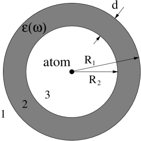
FIG. 1.: Scheme of the spherical cavity.

We apply the formalism developed in Sec. II to the spontaneous decay of an excited two-level atom placed inside a spherical three-layered structure (Fig. 1). The outer layer ($r$ $\!>$ $\!R_{1}$) and the inner layer ($0$ $\!\leq$ $\!r$ $\!<$ $\!R_{2}$) are vacuum, while the middle layer ($R_{2}$ $\!\leq$ $\!r$ $\!\leq$ $\!R_{1}$) is a dispersing and absorbing dielectric. The Green tensor of the configuration is given in Appendix B.

We have performed the calculations assuming a Lorentz-type dielectric with a single resonance (in the relevant frequency region):

$$\epsilon(\omega)=1+{\omega_{\rm P}^{2}\over\omega_{\rm T}^{2}-\omega^{2}-i\omega\gamma}\,.$$ (72)

Here, $\omega_{\rm P}$ is the plasma frequency, which is proportional to the square root of the number density of the Lorentz oscillators and plays the role of the coupling constant between the medium polarization and the electromagnetic field, and $\omega_{\rm T}$ and $\gamma$, respectively, are the position and the width of the medium resonance. The plots in Fig. 2 of the real and imaginary parts of the index of refraction

$$n(\omega)=\sqrt{\epsilon(\omega)}=n_{\rm R}(\omega)+in_{\rm I}(\omega)$$ (73)

illustrate a typical band-gap behavior of the configuration.

FIG. 2.: (a) The real part $n_{\rm R}(\omega)$ and (b) the imaginary part $n_{\rm I}(\omega)$ of the complex refractive index are shown for $\omega_{\rm P}$ $\!=$ $\!0.5\,\omega_{\rm T}$ and $\gamma$ $\!=$ $\!10^{-4}\,\omega_{\rm T}$ (solid line), $\gamma$ $\!=$ $\!10^{-3}\,\omega_{\rm T}$ (dashed line), and $\gamma$ $\!=$ $\!10^{-2}\,\omega_{\rm T}$ (dotted line). The longitudinal frequency $\omega_{\rm L}$ $\!=$ $\!\sqrt{\omega_{\rm T}^{2}\!+\!\omega_{\rm P}^{2}}$ is $\omega_{\rm L}$ $\!\simeq$ $\!1.12\,\omega_{\rm T}$, and hence $\omega_{\rm L}$ $\!-$ $\!\omega_{\rm T}$ $\!\simeq$ $\!0.12\,\omega_{\rm T}$.

B Weak-coupling regime

In the weak-coupling regime, the excited atomic state decays exponentially [Eq. (44)]. For simplicity let us assume that the atom is positioned at the center of the cavity. From Eqs. (42), (45), (46), and (B31), the cavity-modified decay rate is then found to be

$$A=\bar{A}(\omega_{A})\,A_{0}\,,$$ (74)

where $A_{0}$ is decay rate in free space, Eq. (47), and

$$\bar{A}(\omega)=1+{\rm Re}\,C^{33}_{N}(\omega)\ ,$$ (75)

with $C^{33}_{N}(\omega)$ being given by Eqs. (B15) – (B28). Note that if mode expansion applies, $\bar{A}(\omega)$ would correspond to the change of the density of modes due to the presence of the cavity.

When far from the medium resonance absorption is disregarded and hence the (frequency-independent) refractive index is assumed to be real, then previous results obtained by mode decomposition can be recovered. In particular, for $R_{2}$ $\!\to$ $\!0$ we recognize the decay rate obtained in [22, 26] for microspheres and liquid droplets. However, it should be pointed out that even far from the medium resonance the imaginary part of the refractive index cannot be set equal to zero in general, since the contribution to the decay rate of the nonradiative decay associated with absorption increases $\sim$ $\!R_{2}^{-3}$ for decreasing $R_{2}$ (and nonvanishing imaginary part of the refractive index) [11].

FIG. 3.: The function $\bar{A}(\omega)$, Eq. (75), is shown for $R_{2}$ $\!=$ $\!30\,\lambda_{\rm T}$, $d$ $\!=$ $\!\lambda_{\rm T}$, $\omega_{\rm P}$ $\!=$ $\!0.5\,\omega_{\rm T}$, and $\gamma$ $\!=$ $\!10^{-2}\,\omega_{\rm T}$. The curves in the inset correspond to $\gamma=10^{-2}\,\omega_{\rm T}$ (solid line), $\gamma=2\times 10^{-2}\,\omega_{\rm T}$ (dashed line), and $\gamma=5\times 10^{-2}\,\omega_{\rm T}$ (dotted line).

Let us restrict our attention to a true microcavity ($R_{2}\omega_{\rm A}/c$ $\!\gg$ $\!1$). From Fig. 3 it is seen that the rate of spontaneous decay sensitively depends on the transition frequency. Narrow-band enhancement of spontaneous decay ($\bar{A}$ $\!>$ $\!1$) alternates with broadband inhibition ($\bar{A}$ $\!<$ $\!1$). The frequencies where the maxima of enhancement are observed correspond to the resonance frequencies of the cavity. Within the band gap the heights and widths of the frequency intervals in which spontaneous decay is feasible are essentially determined by the material losses. Outside the band-gap zone the change of the decay rate is less pronounced because of the relatively large input–output coupling, the (small) material losses being of secondary importance.

When $R_{2}\omega/c$ $\!\gg$ $\!1$ and $\exp[-n_{\rm I}(R_{1}$ $\!-$ $\!R_{2})\omega/c]$ $\!\ll$ $\!1$, then Eqs. (B15) – (B28) drastically simplify and $\bar{A}(\omega)$ [Eq. (75)] reads

$$\bar{A}(\omega)\simeq{\rm Re}\!\left[\frac{n(\omega)-i\tan(R_{2}\omega/c)}{1-in(\omega)\tan(R_{2}\omega/c)}\right].$$ (76)

The positions $\omega_{m}$ of the maxima of $\bar{A}(\omega)$ can then be obtained from the equation $d\bar{A}/d\omega$ $\!=$ $\!0$. As long as $n(\omega)$ can be regarded as being slowly varying compared with $\tan(\omega R_{2}/c)$, we may neglect $dn/d\omega$ and thus determine the resonance frequencies from the equation

$$2n_{\rm I}(\omega_{m})\,\tan(R_{2}\omega_{m}/c)$$ (78)

$$\hskip 8.61108pt\simeq\,|n(\omega_{m})|^{2}\!-\!1\!-\!\sqrt{(|n(\omega_{m})|^{2}\!-\!1)^{2}\!+\!4n_{\rm I}^{2}(\omega_{m})}\,.$$

Note that Eq. (78) is exact when it is regarded as conditional equation of $R_{2}$ for a desired resonance frequency.

In the band-gap zone we may assume that $n_{\rm I}$ $\!\gg$ $\!n_{\rm R}$ (see Fig. 2). From Eqs. (76) and (78) it then follows that the maximum values $\bar{A}(\omega_{m})$ and half widths at half maximum, $\delta\omega_{m}$, of the cavity resonance lines, i.e., the regions where enhanced spontaneous decay can be observed, are given by

$$\bar{A}(\omega_{m})\simeq{n_{\rm I}^{2}(\omega_{m})+1\over n_{\rm R}(\omega_{m})}\simeq\frac{2\sqrt{(\omega_{\rm L}^{2}-\omega_{m}^{2})(\omega_{m}^{2}-\omega_{\rm T}^{2})}}{\gamma\omega_{m}}\,,$$ (79)

$$\delta\omega_{m}\simeq{c\over R_{2}\bar{A}(\omega_{m})}\,,$$ (80)

where we have assumed that the material losses are small, i.e., $\gamma$ $\!\ll$ $\!\omega_{\rm T},\,\omega_{\rm P},\,\omega_{\rm P}^{2}/\omega_{\rm T}$. Equations (79) and (80) reveal that in the approximation made the heights (widths) of the resonance lines (Lorentzians) are proportional (inversely proportional) to $\gamma$, the highest and narrowest line being in the center of the band gap. Note that the product $\bar{A}(\omega_{m})\delta\omega_{m}$ does not depend on $\gamma$.

Outside the band-gap zone the inequality $n_{\rm R}$ $\!\gg$ $\!n_{\rm I}$ is typically valid (see Fig. 2), and thus Eqs. (76) and (78) yield

$$\bar{A}(\omega_{m})\simeq n_{\rm R}(\omega_{m})\simeq\sqrt{\frac{\omega_{\rm L}^{2}-\omega_{m}^{2}}{\omega_{\rm T}^{2}-\omega_{m}^{2}}}\,,$$ (81)

$$\delta\omega_{m}\simeq{c\over R_{2}\bar{A}(\omega_{m})}\,.$$ (82)

The heights and widths of the resonance lines are now seen to be (approximately) independent of $\gamma$. The lines become higher and narrower if $\omega_{m}$ becomes close to $\omega_{\rm T}$.

The widths of the resonance lines are responsible for the damping of intracavity fields. There are two damping mechanisms: photon leakage to the outside of the cavity and photon absorption by the cavity-wall material. From the analysis given above it is seen that the first mechanism is the dominant one outside the band gap where normal dispersion ($dn_{\rm R}/d\omega$ $\!>$ $\!0$) is observed, while the latter dominates inside the band gap where anomalous dispersion ($dn_{\rm R}/d\omega$ $\!<$ $\!0$) is observed. To illustrate this in more detail, we have calculated the amount of radiation energy observed outside the cavity,

$$W=2c\epsilon_{0}\int_{0}^{\infty}dt\int_{0}^{2\pi}d\phi\int_{0}^{\pi}d\theta\,\rho^{2}\sin\theta\,I({\bf r},t)$$ (83)

($\rho$ $\!>$ $\!R_{1}$), and compared it with the emitted energy in free space $W_{0}$ $\!=$ $\!\hbar\omega_{\rm A}$. Assuming without loss of generality that the atomic transition dipole is $z$-oriented and restricting our attention to the relevant far-field contribution, from Eqs. (59) and (61) together with Eq. (B1) and Eqs. (B35) – (B35) we derive (see Appendix C)

$${W\over W_{0}}\simeq\frac{|A^{13}_{N}(\omega_{\rm A})|^{2}}{1+{\rm Re}C^{33}_{N}(\omega_{\rm A})}\,.$$ (84)

Examples of the dependence on the atomic transition frequency of the amount of radiation energy observed outside the cavity are plotted in Fig. 4. It is seen that inside the gap most of the energy emitted by the atom is absorbed by the cavity wall in the course of time, while outside the gap the absorption is (for the chosen values of $\gamma$) much less significant. Note that with increasing value of $\gamma$ the band gap is smoothed a little bit, and thus the fraction of light that escapes from the cavity can increase.

FIG. 4.: The amount of radiation energy $W$, Eq. (84), observed outside the cavity is shown as a function of the atomic transition frequency $\omega_{\rm A}$ for $\gamma=10^{-2}\,\omega_{\rm T}$ (solid line), $\gamma=2\times 10^{-2}\,\omega_{\rm T}$ (dashed line), and $\gamma=5\times 10^{-2}\,\omega_{\rm T}$ (dotted line). The other parameters are the same as in Fig. 3.

C Strong-coupling regime

The strength of the atom-field coupling increases when the atomic transition frequency $\omega_{\rm A}$ approaches a cavity-resonance frequency $\omega_{m}$. In order to gain insight into the strong-coupling regime, let us first consider the limiting case of one cavity-resonance line being involved in the atom-field interaction. Indeed, when $\omega_{\rm A}$ is close to $\omega_{m}$, then contributions from the other resonance lines become small. Using Eqs. (42), (74), and (75), and recalling that $\bar{A}(\omega)$ behaves like a Lorentzian in the vicinity of $\omega_{m}$, we may simplify Eq. (36) to

$$K(t-t^{\prime})\simeq-{A_{0}\over 2\pi}\,\bar{A}(\omega_{m})(\delta\omega_{m})^{2}e^{-i(\omega_{m}-\omega_{\rm A})(t-t^{\prime})}$$ (87)

$$\hskip 64.58313pt\times\,\int_{-\infty}^{+\infty}\!\!d\omega\,\frac{e^{-i(\omega-\omega_{m})(t-t^{\prime})}}{(\omega-\omega_{m})^{2}+(\delta\omega_{m})^{2}}$$

$$\hskip 12.91663pt=-{\textstyle\frac{1}{2}}A_{0}\bar{A}(\omega_{m})\delta\omega_{m}e^{-i(\omega_{m}-\omega_{\rm A})(t-t^{\prime})}e^{-\delta\omega_{m}|t-t^{\prime}|}\,.$$

Substituting this expression into Eq. (34) and differentiating both sides of the resulting equation with regard to time, we arrive at

$$\ddot{C}_{u}(t)+\left[i(\omega_{m}\!-\!\omega_{\rm A})+\delta\omega_{m}\right]\dot{C}_{u}(t)+(\Omega/2)^{2}C_{u}(t)=0$$ (88)

where

$$\Omega=\sqrt{2A_{0}\bar{A}(\omega_{m})\delta\omega_{m}}\,.$$ (89)

Hence we are left, in the approximation made, with a damped-oscillator equation of motion for the upper-state probability amplitude, where $\bar{A}(\omega_{m})$ and $\delta\omega_{m}$, respectively, are given by Eqs. (79) and (80) [or Eqs. (81) and (82)]. Obviously, when $\omega_{A}$ $\!=$ $\omega_{m}$ and

$$\Omega\gg\delta\omega_{m}$$ (90)

(i.e., strong coupling), then damped Rabi oscillations are observed:

$$\left|C_{u}(t)\right|^{2}=e^{-\delta\omega_{m}t}\cos^{2}(\Omega t/2).$$ (91)

Note that in the opposite case where $\Omega$ $\!\ll$ $\!\delta\omega_{m}$ the solution of Eq. (88) is $|C_{u}(t)|^{2}$ $\!=$ $\!e^{-At}$ with $A$ from Eq. (74) for $\omega_{A}$ $\!=$ $\!\omega_{m}$, which is in agreement with Eq. (44). Equations (89) and (90) together with Eqs. (79) and (80) [or Eqs. (81) and (82)] provide us with an easy rule of thumb for deciding whether the strong-coupling regime is realized or not.

FIG. 5.: The temporal evolution of the occupation probability $|C_{u}(t)|^{2}$ of the upper atomic state is shown for $R_{2}$ $\!=$ $\!30\,\lambda_{\rm T}$, $d$ $\!=$ $\!\lambda_{\rm T}$, $\omega_{\rm P}$ $\!=$ $\!0.5\,\omega_{\rm T}$, $\omega_{\rm A}$ $\!=$ $\!1.046448\omega_{\rm T}$, $A_{0}\lambda_{\rm T}/(2c)$ $\!=$ $\!10^{-6}$, and $\gamma$ $\!=$ $\!10^{-4}\,\omega_{\rm T}$ (solid line), $\gamma$ $\!=$ $\!5\times 10^{-4}\,\omega_{\rm T}$ (dashed line), $\gamma$ $\!=$ $\!10^{-3}\,\omega_{\rm T}$ (dotted line). For comparison, the exponential decay in free space is shown (dashed-dotted line).

FIG. 6.: The temporal evolution of the occupation probability $|C_{u}(t)|^{2}$ of the upper atomic state is shown for $d$ $\!=$ $\!\lambda_{\rm T}$, $\omega_{\rm A}$ $\!=$ $\!0.9999\,\omega_{\rm T}$, $A_{0}\lambda_{\rm T}/(2c)$ $\!=$ $\!10^{-5}$, and (a) $\omega_{\rm P}$ $\!=$ $\!3\,\omega_{\rm T}$, $R_{2}$ $\!=$ $\!30.00197\,\lambda_{\rm T}$, (b) $\omega_{\rm P}$ $\!=$ $\!1.5\,\omega_{\rm T}$, $R_{2}$ $\!=$ $\!30.00179\,\lambda_{\rm T}$. The solid lines correspond to the exact solution and the dashed lines to the approximate analytical solution [solution of Eq. (88)] shifted forwards by (a) $A_{0}\Delta$ $\!t=$ $\!0.009$ and (b) $A_{0}\Delta$ $\!t=$ $\!0.02$. For comparison, the exponential decay in free space is shown (dashed-dotted line).

In order to obtain the exact solution to the problem, we have also solved the basic integral equation (37) [together with the kernel function (49)] numerically. Typical examples of the temporal evolution of the occupation probability of the upper atomic state are shown in Fig. 5 for the case where the atomic transition is tuned to the resonance line in the center of the band gap. The figure reveals that with increasing value of the intrinsic damping constant $\gamma$ of the wall material the Rabi oscillations become less pronounced, in agreement with Eqs. (79), (80), (89), and the inequality (90). From Eqs. (79) and (80) it is seen that (in the approximation made there) the product $\bar{A}(\omega_{m})\delta\omega_{m}$ $\!\simeq$ $\!c/R_{2}$ does not vary with $\gamma$, whereas $\delta\omega_{m}$ linearly increases with $\gamma$. According to Eq. (89), $\Omega$ $\!\propto$ $\!\sqrt{\gamma}$ and thus $\Omega/\delta\omega_{m}$ $\!\propto$ $\!1/\sqrt{\gamma}$, i.e., the condition of strong coupling (90) becomes violated with increasing $\gamma$. Physically, increasing $\gamma$ means increasing probability of (irreversible) absorption of the emitted photon by the wall material and therefore reduced probability of (reversible) atom-field energy exchange. It should be mentioned that with increasing $\gamma$ the (very small) probability that the photon (irreversibly) leaves the cavity also increases. Note that the variation of $\gamma$ in Fig. 5 leaves the imaginary part of the refractive index nearly unchanged, $n_{\rm I}$ $\!\simeq$ $\!1.2$, while the (small) real part $n_{\rm R}$ slightly increases with $\gamma$ (see Fig. 2).

The examples of the temporal evolution of the occupation probability of the upper atomic state shown in Fig. 6 refer to the case where the atomic transition is tuned to a resonance line closest to $\omega_{\rm T}$ below the band gap. According to Eqs. (81), (82), (89), and the condition (90), the resonance frequencies close to $\omega_{\rm T}$ are most favorable for realizing the strong-coupling regime in the range of normal dispersion, because of the rising real part of the refractive index [see Fig. 2(a)]. As expected, the strength of the the Rabi oscillations now varies with the plasma frequency $\omega_{\rm P}$ such that they are less pronounced for small values of $\omega_{\rm P}$. Obviously, decreasing $\omega_{\rm P}$ means increasing input-output coupling, i.e., increasing probability that the emitted photon leaves the cavity instead of back-acting upon the atom.

Finally, Fig. 6 presents a comparison between the exact solution, and the approximate analytical solution [solution of Eq. (88)]. To compensate for the short-time inaccuracy of the analytical solution, it is somewhat shifted forward in time. The agreement between the exact solution and the (shifted) analytical solution is quite good. Obviously, Eq. (88) predicts an initial decay somewhat faster than the exact one. In fact, the spontaneous decay is accelerated only gradually under the back-action of the radiated field being multiply reflected at the boundaries [24, 28], and the single-resonance coupling is established only after a certain interval of time. The sharper is the cavity resonance, the shorter is this interval, which is fully confirmed by the figure.

IV Summary and Conclusions

We have developed a formalism for studying spontaneous decay of an excited atom in the presence of arbitrary dispersing and absorbing dielectric bodies. The formalism is based on a source-quantity representation of the electromagnetic field in terms of the Green tensor of the classical problem and appropriately chosen bosonic quantum fields. It replaces the standard concept of mode decomposition which fails for complex permittivity. All relevant information about the bodies such as form and intrinsic dispersion and absorption properties are contained in the Green tensor. It is worth noting that the Green tensor has been available for a large variety of configurations such as planarly, spherically, and cylindrically multilayered media [31].

We have applied the theory to the spontaneous decay of a two-level atom placed at the center of a three-layered spherical microcavity, modeling the wall by a Lorentz dielectric. The formalism has enabled us to study both the range of normal dispersion and the anomalous-dispersion range within the band gap in a unified way. Whereas in the range of normal dispersion the cavity input–output coupling dominates the strength of the atom-field interaction, the dominating effect within the band gap is the photon absorption by the wall material.

In the study of the spherical-cavity problem, we have assumed that the atom is placed at the center of the cavity, which has drastically reduced the mathematical effort, because only the spherical Bessel function of order $n$ $\!=$ $\!1$ contributes to the Green tensor. The price we paid is that the interaction of the atom with cavity excitations of large $n$, which correspond to high-$Q$ whispering gallery modes and concentrate near the surface by repeated internal reflections has not been included in the analysis. Since the complete Green tensor is known, there is of course no obstacle to perform the calculations for an arbitrary position of the atom. In particular, when the atom is near the surface then nonradiative energy transfer from the atom to the absorbing medium can substantially contribute to the process of spontaneous decay. Further investigations are also necessary in order to give a more detailed analysis of the evolution of the emitted radiation, to answer the question of the ratio of photon emission to nonradiative decay, and to extend the theory to multilevel atom-field interactions.

A The Hamiltonian in the dipole and rotating wave approximations

The Hamiltonian (21) can be rewritten as

$$\displaystyle\hat{H}=\hat{H}_{\rm F}+\hat{H}_{\rm A}+\hat{H}_{\rm AF},$$ (A1)

$$\displaystyle\hat{H}_{\rm F}=\int d^{3}{\bf r}\int_{0}^{\infty}d\omega\,\hbar\omega\,\hat{\bf f}^{\dagger}({\bf r},\omega)\cdot\hat{\bf f}({\bf r},\omega),$$ (A2)

$$\displaystyle\hat{H}_{\rm A}=\sum_{\alpha}{\hat{\bf p}_{\alpha}^{2}\over 2m_{\alpha}}+{1\over 2}\int d^{3}{\bf r}\hat{\rho}_{\rm A}({\bf r})\hat{\varphi}_{\rm A}({\bf r}),$$ (A3)

$$\displaystyle\hat{H}_{\rm AF}=-\sum_{\alpha}{q_{\alpha}\over m_{\alpha}}\hat{\bf p}_{\alpha}\cdot\hat{\bf A}({\bf r}_{\alpha})+\int d^{3}{\bf r}\hat{\rho}_{\rm A}({\bf r})\hat{\varphi}({\bf r}),$$ (A4)

where we have ignored the small $\hat{\bf A}^{2}$ term. Note that in the Coulomb gauge $[\hat{\bf p}_{\alpha},\hat{\bf A}]=0$. For a neutral atom with the nucleus being positioned at ${\bf r}_{\rm A}$, the atomic dipole operator reads

$$\hat{\mathchoice{{\hbox{\boldmath$\displaystyle\mu$}}}{{\hbox{\boldmath$\textstyle\mu$}}}{{\hbox{\boldmath$\scriptstyle\mu$}}}{{\hbox{\boldmath$\scriptscriptstyle\mu$}}}}_{\rm A}\equiv\sum_{\alpha}q_{\alpha}(\hat{\bf r}_{\alpha}-{\bf r}_{\rm A})=\sum_{\alpha}q_{\alpha}\hat{\bf r}_{\alpha}\ ,$$ (A5)

and the first term in the interaction part of the Hamiltonian $\hat{H}_{\rm AF}$ takes the form

$$-\sum_{\alpha}{q_{\alpha}\over m_{\alpha}}\hat{\bf p}_{\alpha}\cdot\hat{\bf A}({\bf r}_{\alpha}) \ \simeq\,-\sum_{\alpha}{q_{\alpha}\over i\hbar}\left[\hat{\bf r}_{\alpha},\hat{H}_{\rm A}\right]\cdot\hat{\bf A}({\bf r}_{\rm A})$$ (A7)

$$\ =\,-{1\over i\hbar}\left[\hat{\mathchoice{{\hbox{\boldmath$\displaystyle\mu$}}}{{\hbox{\boldmath$\textstyle\mu$}}}{{\hbox{\boldmath$\scriptstyle\mu$}}}{{\hbox{\boldmath$\scriptscriptstyle\mu$}}}}_{\rm A},\hat{H}_{\rm A}\right]\cdot\hat{\bf A}({\bf r}_{\rm A}),$$

where the dipole approximation has been employed to replace $\hat{\bf A}({\bf r}_{\alpha})$ $\!\rightarrow$ $\!\hat{\bf A}({\bf r}_{\rm A})$ and $\hat{\bf p}_{\alpha}$ $\!=$ $\!(m_{\alpha}/(i\hbar))[\hat{\bf r}_{\alpha},\hat{H}_{\rm A}]$ has been used.

Now we restrict ourselves to a two-state model of an atom with upper state $|u\rangle$ and lower state $|l\rangle$. These are eigenstates of the unperturbed part of the Hamiltonian $\hat{H}_{\rm A}$ with the eigenvalues $\hbar\omega_{u}$ and $\hbar\omega_{l}$, respectively. Then one can write

$$\displaystyle\hat{H}_{\rm A}=\hbar\omega_{u}|u\rangle\langle u|+\hbar\omega_{l}|l\rangle\langle l|,$$ (A8)

$$\displaystyle|u\rangle\langle u|+|l\rangle\langle l|=\hat{I}.$$ (A9)

In this atomic state space, the dipole operator $\hat{\mathchoice{{\hbox{\boldmath$\displaystyle\mu$}}}{{\hbox{\boldmath$\textstyle\mu$}}}{{\hbox{\boldmath$\scriptstyle\mu$}}}{{\hbox{\boldmath$\scriptscriptstyle\mu$}}}}_{\rm A}$ has the matrix elements $\langle u|\hat{\mathchoice{{\hbox{\boldmath$\displaystyle\mu$}}}{{\hbox{\boldmath$\textstyle\mu$}}}{{\hbox{\boldmath$\scriptstyle\mu$}}}{{\hbox{\boldmath$\scriptscriptstyle\mu$}}}}_{\rm A}|l\rangle=\langle l|\hat{\mathchoice{{\hbox{\boldmath$\displaystyle\mu$}}}{{\hbox{\boldmath$\textstyle\mu$}}}{{\hbox{\boldmath$\scriptstyle\mu$}}}{{\hbox{\boldmath$\scriptscriptstyle\mu$}}}}_{\rm A}|u\rangle\equiv\mathchoice{{\hbox{\boldmath$\displaystyle\mu$}}}{{\hbox{\boldmath$\textstyle\mu$}}}{{\hbox{\boldmath$\scriptstyle\mu$}}}{{\hbox{\boldmath$\scriptscriptstyle\mu$}}}$ and $\langle u|\hat{\mathchoice{{\hbox{\boldmath$\displaystyle\mu$}}}{{\hbox{\boldmath$\textstyle\mu$}}}{{\hbox{\boldmath$\scriptstyle\mu$}}}{{\hbox{\boldmath$\scriptscriptstyle\mu$}}}}_{\rm A}|u\rangle=\langle l|\hat{\mathchoice{{\hbox{\boldmath$\displaystyle\mu$}}}{{\hbox{\boldmath$\textstyle\mu$}}}{{\hbox{\boldmath$\scriptstyle\mu$}}}{{\hbox{\boldmath$\scriptscriptstyle\mu$}}}}_{\rm A}|l\rangle=0$. Using them and Eqs. (17), (A7) – (A9), we arrive at

$$-\sum_{\alpha}{q_{\alpha}\over m_{\alpha}}\,\hat{\bf p}_{\alpha}\cdot\hat{\bf A}({\bf r}_{\alpha})$$ (A12)

$$\hskip 21.52771pt\simeq\left(\hat{\sigma}-\hat{\sigma}^{\dagger}\right)\left[\int_{0}^{\infty}d\omega\,{\omega_{\rm A}\over\omega}\underline{\hat{\bf E}}^{\perp}({\bf r}_{\rm A},\omega)-{\rm H.c.}\right]\cdot\mathchoice{{\hbox{\boldmath$\displaystyle\mu$}}}{{\hbox{\boldmath$\textstyle\mu$}}}{{\hbox{\boldmath$\scriptstyle\mu$}}}{{\hbox{\boldmath$\scriptscriptstyle\mu$}}}$$

$$\hskip 21.52771pt\simeq-\left[\hat{\sigma}^{\dagger}\hat{\bf E}^{\perp(+)}({\bf r}_{\rm A})\cdot\mathchoice{{\hbox{\boldmath$\displaystyle\mu$}}}{{\hbox{\boldmath$\textstyle\mu$}}}{{\hbox{\boldmath$\scriptstyle\mu$}}}{{\hbox{\boldmath$\scriptscriptstyle\mu$}}}+{\rm H.c.}\right],$$

where $\hat{\sigma}=|l\rangle\langle u|,\ \hat{\sigma}^{\dagger}=|u\rangle\langle l|$, $\omega_{\rm A}=\omega_{u}-\omega_{l}$, and $\omega=\omega_{\rm A}$ is set in the integral, because of the rotating wave approximation.

In order to deal with the second term in $\hat{H}_{\rm AF}$, we expand $\hat{\rho}_{\rm A}({\bf r})$ in a multi-polar form and retain only the first non-vanishing term

$$\hat{\rho}_{\rm A}({\bf r})\simeq\sum_{\alpha}q_{\alpha}\delta({\bf r}-{\bf r}_{\rm A})$$ (A15)

$$\hskip 34.44434pt-\mathchoice{{\hbox{\boldmath$\displaystyle\nabla$}}}{{\hbox{\boldmath$\textstyle\nabla$}}}{{\hbox{\boldmath$\scriptstyle\nabla$}}}{{\hbox{\boldmath$\scriptscriptstyle\nabla$}}}\cdot\Big{[}\delta({\bf r}-{\bf r}_{\rm A})\sum_{\alpha}q_{\alpha}(\hat{\bf r}_{\alpha}-{\bf r}_{\rm A})\Big{]}$$

$$\hskip 25.83325pt=-\mathchoice{{\hbox{\boldmath$\displaystyle\nabla$}}}{{\hbox{\boldmath$\textstyle\nabla$}}}{{\hbox{\boldmath$\scriptstyle\nabla$}}}{{\hbox{\boldmath$\scriptscriptstyle\nabla$}}}\cdot\delta({\bf r}-{\bf r}_{\rm A})\hat{\mathchoice{{\hbox{\boldmath$\displaystyle\mu$}}}{{\hbox{\boldmath$\textstyle\mu$}}}{{\hbox{\boldmath$\scriptstyle\mu$}}}{{\hbox{\boldmath$\scriptscriptstyle\mu$}}}}_{\rm A}\,.$$

Then we have

$$\int d^{3}{\bf r}\,\hat{\rho}_{\rm A}({\bf r})\hat{\varphi}({\bf r})\simeq-\int d^{3}{\bf r}\,\big{\{}\mathchoice{{\hbox{\boldmath$\displaystyle\nabla$}}}{{\hbox{\boldmath$\textstyle\nabla$}}}{{\hbox{\boldmath$\scriptstyle\nabla$}}}{{\hbox{\boldmath$\scriptscriptstyle\nabla$}}}\cdot[\delta({\bf r}-{\bf r}_{\rm A})\hat{\mathchoice{{\hbox{\boldmath$\displaystyle\mu$}}}{{\hbox{\boldmath$\textstyle\mu$}}}{{\hbox{\boldmath$\scriptstyle\mu$}}}{{\hbox{\boldmath$\scriptscriptstyle\mu$}}}}_{\rm A}]\big{\}}\hat{\varphi}({\bf r})$$ (A19)

$$\hskip 43.05542pt=\int d^{3}{\bf r}[\delta({\bf r}-{\bf r}_{\rm A})\hat{\mathchoice{{\hbox{\boldmath$\displaystyle\mu$}}}{{\hbox{\boldmath$\textstyle\mu$}}}{{\hbox{\boldmath$\scriptstyle\mu$}}}{{\hbox{\boldmath$\scriptscriptstyle\mu$}}}}_{\rm A}]\cdot\mathchoice{{\hbox{\boldmath$\displaystyle\nabla$}}}{{\hbox{\boldmath$\textstyle\nabla$}}}{{\hbox{\boldmath$\scriptstyle\nabla$}}}{{\hbox{\boldmath$\scriptscriptstyle\nabla$}}}\hat{\varphi}({\bf r})\qquad$$

$$\hskip 43.05542pt=-\hat{\mathchoice{{\hbox{\boldmath$\displaystyle\mu$}}}{{\hbox{\boldmath$\textstyle\mu$}}}{{\hbox{\boldmath$\scriptstyle\mu$}}}{{\hbox{\boldmath$\scriptscriptstyle\mu$}}}}_{\rm A}\cdot\hat{\bf E}^{\parallel}({\bf r}_{\rm A})\qquad$$

$$\hskip 43.05542pt\simeq-\left[\hat{\sigma}^{\dagger}\hat{\bf E}^{\parallel(+)}({\bf r}_{\rm A})\cdot\mathchoice{{\hbox{\boldmath$\displaystyle\mu$}}}{{\hbox{\boldmath$\textstyle\mu$}}}{{\hbox{\boldmath$\scriptstyle\mu$}}}{{\hbox{\boldmath$\scriptscriptstyle\mu$}}}+{\rm H.c.}\right],\qquad$$

where integration by parts and Eq. (16) have been employed for deriving the second and the third equation, respectively, and the rotating wave approximation has been used in deriving the forth equation. Combining (A4), (A12), and (A19) gives

$$\hat{H}_{\rm AF}\simeq-\left[\hat{\sigma}^{\dagger}\hat{\bf E}^{(+)}({\bf r}_{\rm A})\cdot\mathchoice{{\hbox{\boldmath$\displaystyle\mu$}}}{{\hbox{\boldmath$\textstyle\mu$}}}{{\hbox{\boldmath$\scriptstyle\mu$}}}{{\hbox{\boldmath$\scriptscriptstyle\mu$}}}+{\rm H.c.}\right].$$ (A20)

Equations (A1), (A2), (A20), and a subtraction of $(\hbar/2)(\omega_{u}+\omega_{l})\hat{I}$ from $\hat{H}_{\rm A}$, Eq. (A8), lead to the Hamiltonian (25).

B The Green tensor of the spherical cavity

Following[31, 34], we write the Green tensor of the cavity in Fig. 1 in the form

$$\mathchoice{{\hbox{\boldmath$\displaystyle G$}}}{{\hbox{\boldmath$\textstyle G$}}}{{\hbox{\boldmath$\scriptstyle G$}}}{{\hbox{\boldmath$\scriptscriptstyle G$}}}({\bf r},{\bf r^{\prime}},\omega)=\mathchoice{{\hbox{\boldmath$\displaystyle G$}}}{{\hbox{\boldmath$\textstyle G$}}}{{\hbox{\boldmath$\scriptstyle G$}}}{{\hbox{\boldmath$\scriptscriptstyle G$}}}^{\rm V}({\bf r},{\bf r^{\prime}},\omega)\delta_{fs}+\mathchoice{{\hbox{\boldmath$\displaystyle G$}}}{{\hbox{\boldmath$\textstyle G$}}}{{\hbox{\boldmath$\scriptstyle G$}}}{{\hbox{\boldmath$\scriptscriptstyle G$}}}^{(fs)}({\bf r},{\bf r^{\prime}},\omega),$$ (B1)

where $\mathchoice{{\hbox{\boldmath$\displaystyle G$}}}{{\hbox{\boldmath$\textstyle G$}}}{{\hbox{\boldmath$\scriptstyle G$}}}{{\hbox{\boldmath$\scriptscriptstyle G$}}}^{\rm V}({\bf r},{\bf r^{\prime}},\omega)$ represents the contribution of the direct waves from the radiation sources in an unbounded medium, which is vacuum in our case, $f$ and $s$ denote the layers where the field point and source point locate, $\delta_{fs}$ is the usual Kronecker symbol, and the scattering Green tensor $\mathchoice{{\hbox{\boldmath$\displaystyle G$}}}{{\hbox{\boldmath$\textstyle G$}}}{{\hbox{\boldmath$\scriptstyle G$}}}{{\hbox{\boldmath$\scriptscriptstyle G$}}}^{(fs)}({\bf r},{\bf r^{\prime}},\omega)$ describes the contribution of the multiple reflection ($f=s$) and transmission ($f\neq s$) waves. In particular, $\mathchoice{{\hbox{\boldmath$\displaystyle G$}}}{{\hbox{\boldmath$\textstyle G$}}}{{\hbox{\boldmath$\scriptstyle G$}}}{{\hbox{\boldmath$\scriptscriptstyle G$}}}^{(13)}({\bf r},{\bf r^{\prime}},\omega)$ and $\mathchoice{{\hbox{\boldmath$\displaystyle G$}}}{{\hbox{\boldmath$\textstyle G$}}}{{\hbox{\boldmath$\scriptstyle G$}}}{{\hbox{\boldmath$\scriptscriptstyle G$}}}^{(33)}({\bf r},{\bf r^{\prime}},\omega)$ read as [34]

$$\mathchoice{{\hbox{\boldmath$\displaystyle G$}}}{{\hbox{\boldmath$\textstyle G$}}}{{\hbox{\boldmath$\scriptstyle G$}}}{{\hbox{\boldmath$\scriptscriptstyle G$}}}^{(13)}({\bf r},{\bf r^{\prime}},\omega)={ik_{3}\over 4\pi}\sum_{e,o}\sum_{n=1}^{\infty}\sum_{m=0}^{n}$$ (B5)

$$\hskip 34.44434pt\times\Biggl{\{}\frac{2n\!+\!1}{n(n\!+\!1)}\frac{(n\!-\!m)!}{(n\!+\!m)!}(2\!-\!\delta_{0m})$$

$$\hskip 34.44434pt\times\biggl{[}A^{13}_{M}(\omega){\bf M}^{(1)}_{{e\atop o}nm}({\bf r},k_{1}){\bf M}_{{e\atop o}nm}({\bf r}^{\prime},k_{3})$$

$$\hskip 34.44434pt+A^{13}_{N}(\omega){\bf N}^{(1)}_{{e\atop o}nm}({\bf r},k_{1}){\bf N}_{{e\atop o}nm}({\bf r}^{\prime},k_{3})\biggr{]}\Biggr{\}}\ ,$$

$$\mathchoice{{\hbox{\boldmath$\displaystyle G$}}}{{\hbox{\boldmath$\textstyle G$}}}{{\hbox{\boldmath$\scriptstyle G$}}}{{\hbox{\boldmath$\scriptscriptstyle G$}}}^{(33)}({\bf r},{\bf r^{\prime}},\omega)={ik_{3}\over 4\pi}\sum_{e,o}\sum_{n=1}^{\infty}\sum_{m=0}^{n}$$ (B9)

$$\hskip 34.44434pt\times\Biggl{\{}\frac{2n\!+\!1}{n(n\!+\!1)}\frac{(n\!-\!m)!}{(n\!+\!m)!}(2\!-\!\delta_{0m})$$

$$\hskip 34.44434pt\times\biggl{[}C^{33}_{M}(\omega){\bf M}_{{e\atop o}nm}({\bf r},k_{1}){\bf M}_{{e\atop o}nm}({\bf r}^{\prime},k_{3})$$

$$\hskip 34.44434pt+C^{33}_{N}(\omega){\bf N}_{{e\atop o}nm}({\bf r},k_{1}){\bf N}_{{e\atop o}nm}({\bf r}^{\prime},k_{3})\biggr{]}\Biggr{\}}\ ,$$

where

$$k_{1}=k_{3}={\omega\over c},\qquad k_{2}=\sqrt{\epsilon(\omega)}\,{\omega\over c}\,$$

and ${\bf M}$ and ${\bf N}$ represent TM- and TE-waves, respectively,

$${\bf M}_{{e\atop o}nm}({\bf r},k) =\mp{m\over\sin\theta}j_{n}(kr)P_{n}^{m}(\cos\theta){\sin\choose\cos}(m\phi){\bf e}_{\theta}$$ (B11)

$$-j_{n}(kr)\frac{dP_{n}^{m}(\cos\theta)}{d\theta}{\cos\choose\sin}(m\phi){\bf e}_{\phi}\ ,$$

$${\bf N}_{{e\atop o}nm}({\bf r},k) ={n(n+1)\over kr}j_{n}(kr)P_{n}^{m}(\cos\theta){\cos\choose\sin}(m\phi){\bf e}_{r}$$ (B14)

$$+{1\over kr}\frac{d[rj_{n}(kr)]}{dr}\Biggl{[}\frac{dP_{n}^{m}(\cos\theta)}{d\theta}{\cos\choose\sin}(m\phi){\bf e}_{\theta}$$

$$\mp{m\over\sin\theta}P_{n}^{m}(\cos\theta){\sin\choose\cos}(m\phi){\bf e}_{\phi}\Biggr{]},$$

with $j_{n}(x)$ being the spherical Bessel function of the first kind and $P_{n}^{m}(x)$ being the associated Legendre function. The superscript ${(1)}$ in Eq. (B5) indicates that in Eqs. (B11) and (B14) the spherical Bessel function $j_{n}(x)$ has to be replaced by the first-type spherical Hankel function $h^{(1)}_{n}(x)$.

The coefficients $A^{13}_{M,N}$ and $C^{33}_{M,N}$ in Eqs. (B5) and (B9) are defined by

$$A^{13}_{M,N}(\omega) =\frac{T_{F1}^{M,N}T_{F2}^{M,N}T_{P1}^{M,N}}{T_{P1}^{M,N}+T_{F1}^{M,N}R_{P1}^{M,N}R_{F2}^{M,N}}\ ,$$ (B15)

$$C^{33}_{M,N}(\omega) ={A^{13}_{M,N}\over T_{P2}^{M,N}}\left[{R_{P2}^{M,N}\over T_{F1}^{M,N}}+{R_{P1}^{M,N}\over T_{P1}^{M,N}}\right],$$ (B16)

where

$$R^{M}_{Pf} =\frac{k_{f+1}H^{\prime}_{(f+1)f}H_{ff}-k_{f}H^{\prime}_{ff}H_{(f+1)f}}{k_{f+1}J_{ff}H^{\prime}_{(f+1)f}-k_{f}J^{\prime}_{ff}H_{(f+1)f}},$$ (B17)

$$R^{M}_{Ff} =\frac{k_{f+1}J^{\prime}_{(f+1)f}J_{ff}-k_{f}J^{\prime}_{ff}J_{(f+1)f}}{k_{f+1}J^{\prime}_{(f+1)f}H_{ff}-k_{f}J_{(f+1)f}H^{\prime}_{ff}},$$ (B18)

$$R^{N}_{Pf} =\frac{k_{f+1}H_{(f+1)f}H^{\prime}_{ff}-k_{f}H_{ff}H^{\prime}_{(f+1)f}}{k_{f+1}J^{\prime}_{ff}H_{(f+1)f}-k_{f}J_{ff}H^{\prime}_{(f+1)f}},$$ (B19)

$$R^{N}_{Ff} =\frac{k_{f+1}J_{(f+1)f}J^{\prime}_{ff}-k_{f}J_{ff}J^{\prime}_{(f+1)f}}{k_{f+1}J_{(f+1)f}H^{\prime}_{ff}-k_{f}J^{\prime}_{(f+1)f}H_{ff}},$$ (B20)

$$T^{M}_{Pf} =\frac{k_{f+1}\left(J_{(f+1)f}H^{\prime}_{(f+1)f}-J^{\prime}_{(f+1)f}H_{(f+1)f}\right)}{k_{f+1}J_{ff}H^{\prime}_{(f+1)f}-k_{f}J^{\prime}_{ff}H_{(f+1)f}},$$ (B21)

$$T^{M}_{Ff} =\frac{k_{f+1}\left(J^{\prime}_{(f+1)f}H_{(f+1)f}-J_{(f+1)f}H^{\prime}_{(f+1)f}\right)}{k_{f+1}J^{\prime}_{(f+1)f}H_{ff}-k_{f}J_{(f+1)f}H^{\prime}_{ff}},$$ (B22)

$$T^{N}_{Pf} =\frac{k_{f+1}\left(J^{\prime}_{(f+1)f}H_{(f+1)f}-J_{(f+1)f}H^{\prime}_{(f+1)f}\right)}{k_{f+1}J^{\prime}_{ff}H_{(f+1)f}-k_{f}J_{ff}H^{\prime}_{(f+1)f}},$$ (B23)

$$T^{N}_{Ff} =\frac{k_{f+1}\left(J_{(f+1)f}H^{\prime}_{(f+1)f}-J^{\prime}_{(f+1)f}H_{(f+1)f}\right)}{k_{f+1}J_{(f+1)f}H^{\prime}_{ff}-k_{f}J^{\prime}_{(f+1)f}H_{ff}}$$ (B24)

with

$$J_{il} =j_{n}(k_{i}R_{l}),$$ (B25)

$$H_{il} =h^{(1)}_{n}(k_{i}R_{l}),$$ (B26)

$$J^{\prime}_{il} ={1\over\rho}{d[\rho j_{n}(\rho)]\over d\rho}\bigg{|}_{\rho=k_{i}R_{l}},$$ (B27)

$$H^{\prime}_{il} ={1\over\rho}{d[\rho h^{(1)}_{n}(\rho)]\over d\rho}\bigg{|}_{\rho=k_{i}R_{l}}.$$ (B28)

Note that $A^{13}_{M,N}$ and $C^{33}_{M,N}$ are functions of $n$ but not of $m$. When the atom is positioned at the cavity center, we have [11]

$${\bf M}_{{e\atop o}nm}({\bf r},k)\Big{|}_{kr\rightarrow 0}\longrightarrow(kr)^{n},$$ (B29)

$${\bf N}_{{e\atop o}nm}({\bf r},k)\Big{|}_{kr\rightarrow 0}\longrightarrow(kr)^{n-1}.$$ (B30)

In this case, only TM-waves with $n$ $\!=$ $\!1$ contribute and the Eq. (B9) simplifies to

$$\mathchoice{{\hbox{\boldmath$\displaystyle G$}}}{{\hbox{\boldmath$\textstyle G$}}}{{\hbox{\boldmath$\scriptstyle G$}}}{{\hbox{\boldmath$\scriptscriptstyle G$}}}^{\rm R}\equiv\mathchoice{{\hbox{\boldmath$\displaystyle G$}}}{{\hbox{\boldmath$\textstyle G$}}}{{\hbox{\boldmath$\scriptstyle G$}}}{{\hbox{\boldmath$\scriptscriptstyle G$}}}^{(33)}({\bf r},{\bf r^{\prime}},\omega)\Big{|}_{r=r^{\prime}\rightarrow 0}={i\omega\over 6\pi c}C^{33}_{N}(\omega)\mathchoice{{\hbox{\boldmath$\displaystyle I$}}}{{\hbox{\boldmath$\textstyle I$}}}{{\hbox{\boldmath$\scriptstyle I$}}}{{\hbox{\boldmath$\scriptscriptstyle I$}}}.$$ (B31)

Similarly, Eq. (B5) reduces to

$$G^{(13)}_{rz}({\bf r},{\bf r^{\prime}},\omega)\Big{|}_{r^{\prime}\rightarrow 0}={i\cos\theta\over 2\pi r}h_{1}^{(1)}(k_{3}r)A^{13}_{N}(\omega),$$ (B35)

$$G^{(13)}_{\theta z}({\bf r},{\bf r^{\prime}},\omega)\Big{|}_{r^{\prime}\rightarrow 0}=-{i\sin\theta\over 4\pi r}{d[rh_{1}^{(1)}(k_{3}r)]\over dr}A^{13}_{N}(\omega),$$

$$G^{(13)}_{\phi z}({\bf r},{\bf r^{\prime}},\omega)\Big{|}_{r^{\prime}\rightarrow 0}=0.$$

C Derivation of Eq. (84)

For an atom at the cavity center and $z$-oriented dipole, from Eqs. (61) and (B35) – (B35) we derive

$$F_{r}({\bf r},{\bf r}_{\rm A},\omega_{\rm A})={\cal O}(\rho^{-2}),$$ (C1)

$$F_{\theta}({\bf r},{\bf r}_{\rm A},\omega_{\rm A})=-{k_{\rm A}^{2}\mu\sin\theta\over 4\pi^{2}\epsilon_{0}\rho}$$ (C3)

$$\hskip 8.61108pt\times\int_{0}^{\infty}\!\!d\omega\ {\rm Im}\!\left[A^{13}_{N}(\omega)e^{i\omega\rho/c}\right]\zeta(\omega_{\rm A}\!-\!\omega)+{\cal O}(\rho^{-2}),$$

$$F_{\phi}({\bf r},{\bf r}_{\rm A},\omega_{\rm A})=0.$$ (C4)

Recalling the relation $\zeta(x)$ $\!=$ $\!i/(x+i0)$, we perform the $\omega$-integration in Eq. (C3) to obtain

$$\int_{0}^{\infty}d\omega\,{\rm Im}\!\left[A^{13}_{N}(\omega)e^{i\omega\rho/c}\right]\zeta(\omega_{\rm A}-\omega)$$ (C7)

$$\hskip 21.52771pt=-{1\over 2}\int_{0}^{\infty}d\omega\,\frac{\left\{A^{13}_{N}(\omega)e^{i\omega\rho/c}-{\rm c.c.}\right\}}{\omega-(\omega_{\rm A}+i0)}$$

$$\hskip 21.52771pt\simeq-i\pi A^{13}_{N}(\omega_{\rm A})e^{i\omega_{\rm A}\rho/c},$$

where we have (approximately) replaced $A^{13}_{N}(\omega)$ by $A^{13}_{N}(\omega_{\rm A})$, extended the lower limit of the integral to $-\infty$, and applied contour-integration techniques. Combining Eqs. (59), (61), (83), (C1), (C4), and (C7), it is not difficult to prove that

$$W\simeq\hbar\omega_{\rm A}\,\frac{|A^{13}_{N}(\omega_{\rm A})|^{2}}{1+{\rm Re}C^{33}_{N}(\omega_{\rm A})}\,.$$ (C8)

Taking into account that the free-space value $W_{0}$ $\!=$ $\!\hbar\omega_{\rm A}$ is obtained by setting $A^{13}_{N}$ $\!=$ $\!1$ and $C^{33}_{N}$ $\!=$ $\!0$, Eq. (C8) just yields Eq. (84).

REFERENCES

• [1] on leave from the Institute of Physics, National Center for Sciences and Technology, 1 Mac Dinh Chi St., Dist. 1, Ho Chi Minh city, Vietnam.
• [2] Cavity Quantum Electrodynamics, edited by P. R. Berman (Academic, New York, 1994).
• [3] E. A. Hinds, in Advances in Atomic, Molecular, and Optical Physics, edited by D. Bates and B. Bederson (Academic, New York, 1991), Vol. 28, p. 237.
• [4] M. I. Gorodetsky, A. A. Savchenkov, and V. S. Ilchenko, Opt. Lett. 21, 453 (1996).
• [5] S. M. Barnett, B. Huttner, and R. Loudon, Phys. Rev. Lett. 68, 3698 (1992); S. M. Barnett, B. Huttner, R. Loudon, and R. Matloob, J. Phys. B 29, 3763 (1996).
• [6] Y. Lee and M. Yamanishi, Phys. Rev. A 52, 2312 (1995).
• [7] G. Juzeliūnas, Phys. Rev. A 55, R4015 (1997).
• [8] M. S. Tomaš and Z. Lenac, Phys. Rev. A 56, 4197 (1997).
• [9] A. Tip, Phys. Rev. A 57, 4818 (1998).
• [10] S. Scheel, L. Knöll, D.-G. Welsch, and S. M. Barnett, Phys. Rev. A 60, 1590 (1999).
• [11] S. Scheel, L. Knöll, and D.-G. Welsch, Phys. Rev. A 60, 4094 (1999).
• [12] M. Fleischhauer, Phys. Rev. A 60, 2534 (1999).
• [13] S. D. Gupta and G. S. Agarwal, Opt. Commun. 115, 597 (1995).
• [14] M. S. Tomaš and Z. Lenac, Phys. Rev. A 60, 2431 (1999).
• [15] T. Gruner and D.-G. Welsch, Phys. Rev. A 53, 1818 (1996).
• [16] R. Matloob, R. Loudon, S. M. Barnett, and J. Jeffers, Phys. Rev. A 52, 4823 (1995); R. Matloob and R. Loudon, ibid. 53, 4567 (1997).
• [17] Ho Trung Dung, L. Knöll, and D.-G. Welsch, Phys. Rev. A 57, 3931 (1998).
• [18] S. Scheel, L. Knöll, and D.-G. Welsch, Phys. Rev. A 58, 700 (1998).
• [19] V. B. Braginsky, M. L. Gorodetsky, and V. S. Ilchenko, Phys. Lett. A 137, 393 (1989).
• [20] V. Sandoghdar, F. Treussart, J. Hare, V. Lefèvre-Seguin, J.-M. Raimond, and S. Haroche, Phys. Rev. A 54, R1777 (1996).
• [21] D. W. Vernooy, A. Furusawa, N. Ph. Georgiades, V. S. Ilchenko, and H. J. Kimble, Phys. Rev. A 57, R2293 (1998).
• [22] H. Chew, J. Chem. Phys. 87, 1355 (1987); Phys. Rev. A 38, 3410 (1988); S. C. Ching, H. M. Lai, and K. Young, J. Opt. Soc. Am. B 4, 2004 (1987); K. G. Sullivan and D. G. Hall, Phys. Rev. A 50, 2708 (1994); W. Jhe and J. W. Kim, Phys. Rev. A 51, 1150 (1995); W. Jhe and K. Jang, Phys. Rev. A 53, 1126 (1996); V. V. Klimov, M. Ducloy, and V. S. Letokhov, J. Mod. Opt. 43, 549 (1996); ibid 43, 2251 (1996).
• [23] H-B. Lin, J. D. Eversole, C. D. Merritt, and A. J. Campillo, Phys. Rev. A 45, 6756 (1992). M. D. Barnes, C-Y. Kung, W. B. Whitten, J. M. Ramsey, S. Arnold, and S. Holler, Phys. Rev. Lett. 76, 3931 (1996); H. Fujiwara, K. Sasaki, and H. Masuhara, J. App. Phys. 85, 2052 (1999); H. Yukawa, S. Arnold, and K. Miyano, Phys. Rev. A 60, 2491 (1999).
• [24] J. Parker and C. R. Stroud, Phys. Rev. A 35, 4226 (1987).
• [25] H. M. Lai, P. T. Leung, and K. Young, Phys. Rev. A 37, 1597 (1988); D. Lenstra, G. Kurizki, L. D. Bakalis and K. Banaszek, Phys. Rev. A 54, 2690 (1996); V. V. Klimov, V. S. Letokhov, and M. Ducloy, Phys. Rev. A 56, 2308 (1997); V. V. Klimov, M. Ducloy, and V. S. Letokhov, Phys. Rev. A 59, 2996 (1999).
• [26] Fam Le Kien, Nguyen Hong Quang, and K. Hakuta, Opt. Commun., to appear.
• [27] W. H. Press, S. A. Teukolsky, W. T. Vetterling, and B. P. Flannery, Numerical recipes in FORTRAN: the art of scientific computing (Cambridge University Press, Cambridge, England, 1992), p. 786.
• [28] R. J. Cook and P. W. Milonni, Phys. Rev. A 35, 5081 (1987).
• [29] X. P. Feng and K. Ujihara, IEEE J. Quantum Electron. QE-25, 2332 (1989).
• [30] Ho Trung Dung and K. Ujihara, Phys. Rev. A 60, 4067 (1999).
• [31] W. C. Chew, Waves and Fields in Inhomogeneous Media (IEEE Press, New York, 1995).
• [32] A. A. Abrikosov, L. P. Gorkov, and I. E. Dzyaloshinski, Methods of Quantum Field Theory in Statistical Physics (Dover, New York, 1975).
• [33] W. Vogel and D.–G. Welsch, Lectures on Quantum Optics (Akademie Verlag, Berlin, Germany, 1994), pp. 212.
• [34] L. W. Li, P. S. Kooi, M. S. Leong, and T. S. Yeo, IEEE Trans. Microwave Theory Tech. 42, 2302 (1994).