Comparing Protein Interaction Networks via a Graph Match-and-Split Algorithm

Abstract

We present a method that compares the protein interaction networks of two species to detect functionally similar (conserved) protein modules between them. The method is based on an algorithm we developed to identify matching subgraphs between two graphs. Unlike previous network comparison methods, our algorithm has provable guarantees on correctness and efficiency. Our algorithm framework also admits quite general connectivity and local matching criteria that define when two subgraphs match and constitute a conserved module.

We apply our method to pairwise comparisons of the yeast protein network with the human, fruit fly and nematode worm protein networks, using a lenient criterion based on connectedness and matching edges, coupled with a betweenness clustering heuristic. We evaluate the detected conserved modules against reference yeast protein complexes using sensitivity and specificity measures. In these evaluations, our method performs competitively with and sometimes better than two previous network comparison methods. Further under some conditions (proper homolog and species selection), our method performs better than a popular single-species clustering method. Beyond these evaluations, we discuss the biology of a couple of conserved modules detected by our method. We demonstrate the utility of network comparison for transferring annotations from yeast proteins to human ones, and validate the predicted annotations.

1 Introduction

Making sense of it all.

Protein-protein interactions are the basis of many processes that maintain cellular structure and function. Organizing the myriad protein interactions in a cell into functional modules of proteins is a natural step in exploring these cellular processes [12]. The need for such organization is readily evident from a glance at the network of interactions observed in the yeast Saccharomyces cerevisiae (Figure 1). Numerous such interactions are publicly available for other organisms too from high-throughput though noisy experiments or extensive literature scanning [5]. Computational methods are valuable to make sense of this raw data and cope with its scale. These methods are similar in spirit to ones that organize raw genomic sequences into functional elements like genes, regulatory sequences, etc.

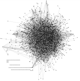
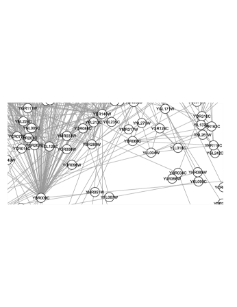
Figure 1: Global view of the protein interaction network of Saccharomyces cerevisiae (left) comprising $14,319$ interactions over $4389$ proteins, and a zoomed view of some proteins (right). A dot or circle represents a protein and a line joins two interacting proteins. The protein networks in this paper are drawn using the Cytoscape software [21].

In this work, a protein (interaction) network refers to a graph whose nodes are the proteins of an organism and edges indicate physical interactions between proteins, and a protein module refers to a subset of proteins in this network along with the interactions between them. A functional module is then a protein module known or supposed to be involved in a common cellular process (eg. a protein complex or a signaling pathway). Note however that concrete definition of a cellular process is a subject of continuing discussion in biology [12].

Previous work.

Several methods analyse a single organism’s protein network to identify functional modules (see review [5]). A typical single-species method uses connectivity information to cluster a protein network into highly connected modules (eg. MCODE [3]). The method is effective if the modules it outputs align well with a set of reference or known functional modules, and if the output modules that don’t match any known functional module suggest plausible and testable biological hypotheses.

A few recent methods compare protein networks from two or more species to identify functionally similar (conserved) protein modules between them (see review [22]). These pairwise or multiple network comparison methods improve over single-species methods by using information on conservation (cross-species similarity of protein sequences and interaction patterns) as well as connectivity of the networks. For instance amidst noisy data, conservation could reinforce evidence that some connected proteins participate in a common function. These comparative methods also enable transfer of functional annotations between organisms at the level of conserved modules, interactions and proteins, a key utility single-species methods cannot provide. Similarly, conserved modules could provide a basis for studies on the evolution of cellular structures and networks.

Current network comparison methods include NetworkBLAST [23], MaWISh [15], a Bayesian method [4] and Græmlin [9]. At a high level, these methods formulate a biologically-inspired measure to score when a set of subgraphs from the input networks constitute a conserved module and use a greedy heuristic to search for all high-scoring similar subgraphs between the networks. Heuristics are necessary as their complicated scoring measures lead to intractable (NP-hard [10]) search problems.

This work.

We present a pairwise network comparison method based on a graph-matching algorithm with provable guarantees. Our novel graph-matching algorithm and the guarantees on both its correctness and running time makes this work markedly different from previous methods relying on search heuristics. Our search formulation is biologically meaningful and yields promising results in detecting functional modules and transferring functional annotations.

We formulate a conserved protein module as a pair of connected and locally matching subsets of proteins, one from each input network. A locally matching subset pair comprises protein pairs that have similar sequences and similar neighborhood or context in the networks. Search for such conserved modules is simpler than search formulations in previous methods and hence admits an efficient polynomial-time algorithm. The main operation of this algorithm is a recursive match and split of the proteins in the two input networks. We assess the statistical significance of the conserved modules found by the algorithm using similar paths statistics and reliabilities of noisy interactions.

Our polynomial-time search problem is a novel contribution in the broader field of graph-matching as well. Graph-matching refers to a class of problems that find similar subgraphs between two graphs (see [20] for other classes). Many graph-matching problems in literature are NP-hard [10], permitting only heuristic or approximate solutions, due to a stringent global structural match that they require between the similar subgraphs, as opposed to the local match our problem requires. For instance, the maximum common subgraph problem requires an exact isomorphic match between subgraphs and is NP-hard [10]. Problems that require inexact match between graphs to deal with error-prone data are NP-hard too for a family of graph edit cost functions [7]. Some studies use a scoring function to measure how similar two subgraphs are. They find high-scoring subgraph pairs by finding heavy-weight subgraphs in a product graph of the input graphs [23, 15], which is also NP-hard by reduction from the maximum weight induced subgraph [15] or maximum clique problem [10].

2 Methods

2.1 Conserved module premise

Our method compares protein networks from two species to find functionally similar or conserved protein modules between them. A conserved module is intuitively a pair of protein modules that share cross-species similarity at the node level (homology of corresponding protein sequences) and graph structure level (pattern of interactions). Our method’s specific premise is that a conserved module is a pair of connected and locally matching subsets of proteins, one from each input graph. Two proteins locally match if their sequences and neighborhood in the network are similar, and a collection of such protein pairs is a locally matching subset pair. We support this premise in this section and formalize it in the next.

Our premise is biologically motivated. The premise’s connectivity criterion makes it likely for a subset of proteins to be functionally homogeneous and its local matching criterion makes it likely for two protein subsets to be functionally similar. Moreover, these criteria are minimal requirements and hence sensitive in detecting reference functional modules. To illustrate, a functional module’s counterparts in two different species needn’t match exactly in their graph structure due to evolutionary divergence or errors in the interaction data, which makes a local match more sensitive than a stringent structural match like exact isomorphism. The two criteria yield good specificity too with some additional improvements detailed in Section 2.3.1. Note that a method’s sensitivity denotes the fraction of reference modules it detects and specificity the fraction of modules output by it that match some reference module.

Our premise is also computationally attractive as it results in a search problem that admits provably good algorithms for many choices of the connectivity and local matching criteria. As mentioned before in Section 1, our method’s tractable search formulation contrasts it from previous network comparison methods and graph-matching problems.

2.2 Graph-matching engine

Finding conserved modules under the premise just outlined reduces to a graph-matching problem of finding similar subgraphs between two input graphs. We present this graph-matching problem variant and our polynomial-time algorithm for it in this section, keeping formal details to a minimum for reader convenience (see Supplemental text for complete analysis). We also discuss the algorithm’s generality, which makes it relevant for application areas beyond protein networks.

Figure 2: Pictorial sketch of the main operations of our graph-matching algorithm. We show the input graphs $G,H$ and their subgraphs as ovals, hiding node and edge details. The algorithm focuses only on the shaded subgraph pairs at any point in its execution, and refines them recursively until all solutions (similar subgraph pairs) are found. A refinement involves doing a match and a split step to compute locally matching and connected node-sets between two shaded subgraphs (see text for details). The subgraph pair $S_{1},T_{1}$ is a solution, and the algorithm might find more solutions as it recurses on the subgraph pairs $E_{i},F_{j}$. The statistically significant solutions are finally output as conserved modules.

As a prelude, we sketch our graph-matching engine in Figure 2 and informally outline it now in the context of protein networks. Say we start with the yeast and human protein networks along with the homologous protein pairs between them. Our algorithm first computes locally matching proteins between the two networks, and safely discards the other proteins (i.e., any yeast protein with no human homolog or with some human homolog but with poor local match, and vice versa). The algorithm next splits the remaining yeast and human networks into connected sets of proteins. These connected subgraphs are locally matching with respect to the full input networks and contain amongst them the actual solutions with refined local matching relations. To find the solutions, our algorithm repeats the above match and split steps on each pair of the connected subgraphs recursively (as in Figure 2). The ensuing text provides precise descriptions on matching general graphs.

2.2.1 Problem statement

We are given as input two graphs and a node similarity function sim$(.,.)$. The function sim$(u,v)$ is true whenever node $u$ is similar to node $v$ (eg. based on sequence similarity of proteins) and false otherwise. This sim$(.,.)$ is a symmetric function defined over all pairs of nodes $u,v$, one from each input graph. The problem now is to list pairs of connected and locally matching subgraphs between the input graphs. In this work, a subgraph of a graph usually refers to an induced subgraph, which is a subset of nodes in the graph along with all edges between them.

We first build a local-match${}_{S,T}(u,v)$ function for any subgraph pair $S,T$ of the input graphs using the sim$(.,.)$ function. This new function captures local or contextual match between the nodes $u$ of $S$ and $v$ of $T$ using similar local structures present around these nodes in $S$ and $T$. Two possible choices of similar local structures are: similar length-$p$ paths for some small $p$ (say $2$), and $s$-similar neighborhoods around nodes for some small $s$ (see Figure 3). In the former case, local-match${}_{S,T}(u,v)$ is true whenever some length-$p$ path in $S$ containing $u$ is similar to some length-$p$ path in $T$ containing $v$ (two paths are similar if all their corresponding nodes are similar according to sim$(.,.)$). In the latter case, local-match${}_{S,T}(u,v)$ is true whenever sim$(u,v)$ is true and sim$(u^{\prime},v^{\prime})$ is true for at least $s$ distinct neighbor pairs $u^{\prime}$ of $u$ in $S$ and $v^{\prime}$ of $v$ in $T$. The stringency of this criterion increases with $s$, with $1$-similar neighborhoods being the least stringent.

Figure 3: Illustration of two similar local structures (left) and two solutions (right). Assume sim$(u_{i},v_{j})$ is true whenever $u_{i},v_{j}$ have the same label shown inside brackets. The dotted lines (left) show some of the locally matching node pairs. The subgraph pair $S_{1},T_{1}$ is a solution when the local matching criterion is based on similar length-$p$ paths ($p\!=\!1\mbox{ or }2$) or $1$-similar neighborhoods, and $S_{2},T_{2}$ is a solution when the criterion is based also on $2$-similar neighborhoods.

We are ready to state the problem. Given two input graphs $G,H$, a node similarity function sim$(.,.)$, and a local-match${}_{S,T}(.,.)$ function computable for any two subgraphs $S,T$, the problem is to find all maximal induced subgraph pairs $S\subseteq G$, $T\subseteq H$ that satisfy two criteria:

Connectivity: $S,T$ are each connected, and

Local Matching: Each node $u$ in $S$ locally matches at least one node $v$ in $T$ according to the local-match${}_{S,T}(u,v)$ function, and vice versa.

Any subgraph pair that satisfy the above two criteria is called a solution (see Figure 3), and maximality requires that of two solutions $S,T$ and $S^{\prime},T^{\prime}$ with $S^{\prime}\subseteq S,T^{\prime}\subseteq T$, we only output the maximal one $S,T$ to avoid redundancy.

2.2.2 Algorithm and analysis

We present a simple and efficient algorithm for the above problem for any monotone local matching criterion. A monotone criterion is one where any two nodes that locally match remain so even after adding more nodes to the subgraphs under consideration (i.e., if local-match${}_{S,T}(u,v)$ is true, then local-match${}_{S^{\prime},T^{\prime}}(u,v)$ is also true for any $S^{\prime}\supseteq S,T^{\prime}\supseteq T$). The similar length-$p$ paths or $s$-similar neighborhoods criterion from last section are monotone. A useful property of monotonicity is that the maximal solutions are only quadratic in number, since it lets us merge any two solutions $S,T$ and $S^{\prime},T^{\prime}$ with a common node pair $u,v$ (i.e., $u\in S\cap S^{\prime},v\in T\cap T^{\prime}$) into one solution $S\cup S^{\prime},T\cup T^{\prime}$.

Our algorithm presented below matches and splits the nodes of G and H into smaller components, and then recurses on each of the component pairs. For induced subgraphs $S\subseteq G,T\subseteq H$, we let $lm(S,T)$ denote all nodes $u$ in $S$ for which local-match${}_{S,T}(u,v)$ is true for some node $v$ in $T$.

Match-and-Split($G,H$):

[Match] Compute induced subgraph:

$G^{\prime}$ of $G$ over the locally matching nodes $lm(G,H)$, and

$H^{\prime}$ of $H$ over the locally matching nodes $lm(H,G)$.
[Split] Find connected components:

$G_{1},\ldots,G_{c}$ of $G^{\prime}$, and

$H_{1},\ldots,H_{d}$ of $H^{\prime}$.
[Recurse]
if ($c=1,d=1$ and $G^{\prime}=G,H^{\prime}=H$)

Output the maximal solution $G,H$. [base case]
else

for $i=1\mbox{ to }c,j=1\mbox{ to }d$

Match-and-Split($G_{i},H_{j}$). [recursive case]

Correctness.

Consider any solution $S,T$. Each recursive call retains all locally matching nodes and processes all pairs of resulting components. Hence in at least one path of the recursion call tree, all nodes in $S,T$ remain locally matching due to monotonicity and connected as part of a bigger subgraph pair. This retained unsplit $S,T$ is finally output as part of a solution. Further, the output solutions are maximal because no node pair is common to any two output solutions (as shown in the Supplemental text).

Running time.

Let $n_{F},m_{F}$ denote the number of nodes, edges respectively in a graph $F$. The algorithm runs in time $O(n_{G}n_{H}+(n_{G}+n_{H})m_{G}m_{H})$ on the graphs $G,H$ when the local matching criterion is similar length-$1$ paths. This running time bound follows from bounds proved in the Supplemental text, which hold for more general monotone local matching criteria. The algorithm is efficient in practice too as the locally matching proteins between two graphs in our experiments reduces drastically as the recursion depth increases.

2.2.3 Generality of the algorithm

Our algorithm framework admits quite general schemes to search for similar subgraph pairs and score them, and is hence attractive in a biological setting. The searching scheme is flexible as our problem variant and algorithm works for different connectivity and local matching criteria. The scoring scheme is flexible as it is decoupled from the searching scheme. Besides, the number of maximal solutions is only quadratic, so it is not expensive to compute a sophisticated, biologically-inspired score for every solution.

We discuss the flexibility of the local matching and connectivity criteria in more detail. We already saw different monotone local matching criteria. We could also combine such monotone criteria to get a new monotone criterion. For example, declaring two nodes as locally matching if they are so with respect to similar length-$p$ paths or $s$-similar neighborhoods gives a less stringent criterion. Many connectivity criteria are possible too. We could replace connectedness with biconnectedness [2] for instance by simply changing the algorithm’s split step, and still obtain a provably efficient algorithm (see Supplemental text).

2.3 Overall method

Our method of detecting conserved modules between two protein networks involves a searching scheme to find similar subgraph pairs (candidate conserved modules or candidates) using our graph-matching algorithm above, and a scoring scheme to rank these candidates using statistics of similar paths between a subgraph pair. We now describe these schemes and their place in the overall Match-and-Split method.

2.3.1 Searching scheme (via graph-matching)

To adapt the generic graph-matching algorithm Match-and-Split to the specific task of comparing protein networks, we make default choices for certain graph-matching parameters and incorporate a clustering heuristic to handle solutions that are large. In this section, our algorithm’s maximal solutions are referred to simply as solutions.

Choosing parameters.

Our default parameter choices result in a lenient graph-matching criterion, for we would like to detect as many functional modules as possible from noisy protein networks of divergent organisms (eg. yeast and human). The default choices we made on exploring a limited parameter space follow.

Connectedness defines our connectivity criterion. We choose it over biconnectedness as some functional modules (eg. linear signaling pathways) are not biconnected, and even those over highly interacting proteins (eg. protein complexes) may not appear biconnected due to incomplete interaction data.

Similar length-$p$ paths (for $p\!=\!1,2$) defines our local matching criterion. We choose it over $s$-similar neighborhoods (for $s\!=\!1,2$) again on the basis of sensitivity. For $p,s\!=\!1$, both options are equivalent as they yield the same $lm(S,T)$ node-set (defined in Section 2.2.2). However for $p,s\!=\!2$, this node-set from similar paths is a superset of the one from similar neighborhoods, so similar paths is a more lenient criterion.

Sequence similarity defines our node similarity function as in previous network comparison methods. We in fact choose the same criteria used in two previous methods for fair evaluation. The two criteria are: ($A$) sim$(u,v)$ is true whenever the BLAST E-value of proteins $u,v$ is at most $10^{-7}$ and each protein is among the $10$ best BLAST matches of the other [23], and ($B$) sim$(u,v)$ is true whenever the BLAST E-value of $u,v$ is less than that of $60\%$ of ortholog pairs in some ortholog database (see [16] for details).

Incorporating clustering heuristic.

Increased sensitivity from the lenient graph-matching criterion above comes at a cost. Sometimes, a solution is over a large number of proteins and hence less specific. For instance, a solution from a preliminary comparison of yeast and human networks covers more than $500$ yeast and human proteins! To split such large solutions, we incorporate a betweenness clustering heuristic in our Match-and-Split algorithm. This clustering splits a graph into highly-connected, smaller clusters based on iterative computations of an edge betweenness centrality measure [11] (see Supplemental text for details). One could also cluster a graph using other methods such as the popular spectral clustering methods [25].

We incorporate the clustering by replacing our algorithm’s ‘[base-case]’ statement with the code block below. As before $n_{G}$ refers to the number of nodes in $G$, and we may assume $n_{G}\geq n_{H}$ without loss of generality. The parameter $n_{\max}$ (say $25$) indicates when a solution is large.

[base case] code block:
if ($n_{G}\leq n_{\max}$ and $n_{H}\leq n_{\max}$)

Output the maximal solution $G,H$.
else [large solution]

Split $G$ into clusters $G_{1},\ldots,G_{e}$ using betweenness clustering.

for $i=1\mbox{ to }e$

Match-and-Split($G_{i},H$).

A betweenness clustering of $G$ takes $O(n_{G}m_{G}^{2})$ running time [11]. In practice, incorporating the clustering heuristic is not expensive as our experiments result in very few large solutions (mostly one), each covering just a few hundred nodes.

2.3.2 Scoring scheme (via similar paths)

We score a candidate conserved module based on the number of similar length-$p$ paths, and express the statistical significance of the score as a P-value. We use the P-values both to rank the candidates from the searching scheme and to retain only those with P-values at $10\%$ significance level after multiple testing. Our scoring scheme is flexible, as seen in Section 2.2.3, in permitting complicated scoring measures including measures in previous network comparison methods. Still we use a simple scoring measure and the promising results we obtain shows the strength of our searching scheme based on the graph-matching algorithm.

The score of a candidate conserved module $S\subseteq G,T\subseteq H$, where $G,H$ are the input protein networks, is simply the number of pairs of similar length-$p$ paths between them (defined in Section 2.2.1). We evaluate the P-value of this score using a null model that randomizes the edges and node similarity function of $G,H$ to exclude the mechanism of interest viz., conservation of protein modules. To provide a stringent control, the randomization loosely preserves the degree sequence and node similarity distribution as in previous methods. The simplicity of our scoring measure and null model allows us to develop an analytical bound on the P-value (see Supplemental text). This bound can also incorporate reliabilities of noisy protein interactions.

2.3.3 Implementation pipeline and dataset

The overall Match-and-Split method proceeds in a pipeline to detect candidate conserved modules between two protein networks. First our searching scheme uses the novel graph-matching algorithm to produce candidates, then a size filter retains only medium-sized candidates, and finally our scoring scheme ranks the candidates by their P-values and retains those at $10\%$ significance level (after multiple testing). A fast implementation of the method is publicly available (see Supplemental text for website reference), and it takes only a minute or few (at most $4$) on a $3.4$ GHz Pentium Linux machine to compare two studied networks.

The size filter, similar to one in a previous method [23], retains any candidate subgraph pair $S,T$ whose number of nodes $n_{S},n_{T}$ satisfy $n_{\min}\leq n_{S},n_{T}\leq n_{\max}$ ($n_{\min}=3,n_{\max}=25$ in our experiments, and $n_{\max}$ is same as in the searching scheme’s clustering heuristic). We focus on such medium-sized candidates for the following reasons. A large module as a whole is likely to correspond to a less specific function and worse causes artifactual increase in sensitivity in our evaluation studies. A small module, over say two proteins, is likely to result from a spurious match occurring simply by chance.

The protein networks for model organisms Saccharomyces cerevisiae, Drosophila melanogaster and Caenorhabditis elegans (referred hereafter as yeast, fly and worm respectively) are experimentally-derived (eg. two-hybrid, immunoprecipitation) interactions collected in the DIP database [19]. The version of the networks used and the interaction reliabilities based on a logistic regression model are taken from a previous study [23]. Our human protein network is from the HPRD database [18] (binary or direct interactions; Sep 2005 version), and we assume unit reliability for these interactions as they are literature-based.

2.4 Evaluation measures

We describe some measures that we would need in the Results section to evaluate and interpret the conserved modules from pairwise network comparisons. The notation yeast-human comparison denotes the comparison between yeast and human protein networks, and yeast-human modules the resulting conserved modules. Similar notations apply for other two-species comparisons too.

2.4.1 Performance (sensitivity and specificity)

The performance of a pairwise network comparison method depends on the quality of candidate conserved modules it outputs, which we could measure by how well the candidate set aligns with a reference set of conserved modules. But such reference sets, even if available, are not comprehensive or applicable for our purpose (eg. STKE (http://stke.sciencemag.org/cm/, Jun 2005) contains only a couple of fly-worm conserved signaling pathways and no protein complexes; Biocarta (http://www.biocarta.com/genes/allPathways.asp, Jan 2006) has many human-mouse conserved pathways but available mouse interaction data is sparse).

A viable alternative is to use known functional modules in a single species as reference to evaluate part of a candidate set. Our reference modules are the literature-based yeast protein complexes present in MIPS [17] (May 2006 version), at level at most $3$ in its complex category hierarchy. We consider only complexes with $3$ to $25$ proteins due to our study’s focus on medium-sized modules (see Section 2.3.3 for reasons). To test a method, we compare the yeast network against the human, fly or worm network (dataset details in Section 2.3.3), collect the yeast subgraphs $S$ from each output candidate $S,T$, and measure the overlap of these single-species candidate modules with the reference modules.

Our main measures are module-level sensitivity and specificity, which are the fraction of reference modules covered by some candidate module and that of candidate modules covered by some reference module respectively. A module $S$ of proteins from a single species (yeast) is covered by another module $S^{\prime}$ if $|S\cap S^{\prime}|/|S|\geq 50\%$, a stringent criterion given the noisy interaction data.

We also present measures at the interaction and protein levels to assess the quality of different components of candidate modules (similar to measures at the gene, exon and nucleotide levels in gene structure prediction methods [8]). Define the protein interactions spanned by a set of modules as the union of interactions present in each of these modules. If set $A$ denotes the interactions spanned by all candidate modules and $B$ that by all reference modules, then interaction-level sensitivity is $|A\cap B|/|B|$ and specificity is $|A\cap B|/|A|$. Protein-level measures are defined similarly.

2.4.2 GO analysis measures

We use the GO resource [24] for functional annotations of genes. Specifically, all our functional descriptions are based on known GO Biological Process annotations (Aug 2006 version) of proteins to terms at level at least $4$ in the GO hierarchy. Given these annotations, we next define many GO-related concepts that we would need later.

The best GO term of a protein module is the term the module’s proteins are enriched for with the least hypergeometric P-value (computed by GO::TermFinder [6] at $10\%$ significance level with Bonferroni correction). Given two GO terms, the match between them is the overlap $\min(|A\cap B|/|A|,|A\cap B|/|B|)$ between the set $A,B$ of terms they imply, where a GO term implies itself and its ancestors in the GO ontology. This match is based on a well-justified measure [14].

We call a protein module functionally homogeneous if at least $50\%$ of its proteins are annotated with the best GO term the whole module is enriched for. We call a candidate conserved module $S,T$ (eg. yeast-human candidate) as functionally similar with respect to GO if $S$ and $T$ are each functionally homogeneous and the match between their best GO terms is at least $75\%$.

When validating a predicted GO term of a protein, we use a well-justified criterion as for match between terms. This criterion requires the respective sets $A,B$ of terms implied by the predicted term and some known term annotated to the protein to have a high overlap $|A\cap B|/|A|\geq 75\%$.

3 Results

3.1 Performance against previous methods

We test our Match-and-Split method against two previous methods, NetworkBLAST and MaWISh. We try two Match-and-Split versions, $p\!=\!1$ and $p\!=\!2$, which specify the local matching criterion of similar length-$p$ paths. NetworkBLAST has two versions too, a clusters one to detect conserved protein complexes and a paths one to detect conserved paths of length just $4$. We don’t test the Bayesian [4] and Græmlin [9] methods as they are from very recent studies with results focusing on coexpression or prokaryotic networks, whereas the current study’s focus is eukaryotic protein networks. Fundamentally though, all these methods work for the networks of any species.

We evaluate a method by measuring how well the yeast modules it outputs (on pairwise protein network comparisons of yeast and other species) align with a reference set of yeast protein complexes in MIPS, as explained in Section 2.4.1. For fair evaluation, we attempt to use common input, default parameter values, and common output processing for all methods. For instance, the input networks and node similarity function sim$(.,.)$ are the same across methods. The $3,25$ size filter thresholds are same too, so we evaluate all methods only on the medium-sized candidates they output (see Section 2.3.3).

Different sim$(.,.)$ criteria could yield quite varying results, and we try two criteria used in previous methods as discussed in Section 2.3.1. The main text presents criterion $A$ results as every method has better or comparable module-level results with criterion $A$ than $B$. The Supplemental text has some criterion $B$ results to show few departures from this trend (mainly in yeast-worm comparison and minor increase of MaWISh specificity in yeast-human case) and indicate slight changes in the relative performance of the methods between the two criteria.

First, we discuss module-level results of Match-and-Split ($p\!=\!1$) relative to the other two methods. In yeast-human comparison (Table 1), Match-and-Split and MaWISh have comparable performance with Match-and-Split being somewhat better. A similar trend appears in the yeast-fly case (Table 2) and with an exception in the yeast-worm case (Table 1 of the Supplemental text). In all three cases, NetworkBLAST (clusters) has better sensitivity than other methods at the cost of very low specificity. NetworkBLAST (paths) achieves better sensitivity and reasonable specificity, but only by outputting too many and too small ($4$-protein) candidates. The small size permits a brute-force search for optimal candidates, which is better than the greedy heuristic search for larger candidates in NetworkBLAST (clusters). In contrast, the search in Match-and-Split is based on a provably efficient graph-matching algorithm with no candidate size restrictions.

Moving from relative to absolute performance, the values of module-level sensitivity and specificity are low (for example, a mere $25.0\%$ and $47.5\%$ respectively by Match-and-Split ($p\!=\!1$), a competitive method in yeast-human case). Low sensitivity could be due to factors like noisy interaction data, poor conservation of complexes across compared organisms, or differing computational and biological definitions of a functional module or complex. Finding which of these factors is key is a subject of future work. Low specificity is probably due to incompleteness of the reference set, and it does not indicate the output candidates are spurious (a claim supported by further analysis in Section 3.4).

3.2 Single-species vs pairwise network analysis

Pairwise network comparison methods use cross-species conservation in an attempt to improve over single-species methods in detection of functional modules (as seen in Section 1). But previous network comparison studies have not evaluated their methods against single-species ones. Here we undertake this evaluation by testing a popular single-species method MCODE [3] on the yeast network under the same measures and size range ($3$ to $25$ proteins) as before. It is beyond the scope of this study to test all single-species methods.

The performance of the pairwise methods relative to the single-species MCODE is varied. Under proper homolog and species selection, Match-and-Split performs better than MCODE in detecting reference yeast complexes. Comparing Table 1 on yeast-human comparison with Table 3, Match-and-Split ($p\!=\!1$) is much more sensitive than MCODE at the same specificity, and MaWISh performs similar to MCODE. The choice of homologs is important as changing the sim$(.,.)$ criterion from $A$ here to $B$ in Table 2 of the Supplemental text reduces the benefit of pairwise methods over MCODE. Species selection is also crucial as the pairwise methods have worse sensitivity than MCODE in the yeast-fly (Table 2) and yeast-worm (Table 1 of the Supplemental text) cases. Low sensitivity in the yeast-worm case could be due to the sparse worm interaction data, but the reason in the yeast-fly case is unclear as the fly network is interaction-rich.

Method	# output modules	Module		Interaction		Protein
	(interactions, proteins)	Sens.	Spec.	Sens.	Spec.	Sens.	Spec.
Match-and-Split
($p\!=\!1$)	80 (667, 421)	25.0	47.5	20	35	25	48
($p\!=\!2$)	72 (664, 411)	28.0	41.7	20	34	25	47
NetworkBLAST
(clusters)	66 (1042, 522)	32.6	18.2	30	33	33	50
(paths, length 4)	276 (625, 563)	28.0	48.2	18	33	34	48
MaWISh	151 (508, 389)	20.5	43.7	15	33	23	46

Table 1: Evaluation of output candidates from yeast-human network comparison using sensitivity (sens.) and specificity (spec.) measures (expressed as rounded percentages) at the module, interaction and protein levels. The second column shows the number of yeast modules (candidates) output, and the number of interactions and proteins spanned by these yeast modules. The reference set comprises $132$ medium-sized (size 3 to 25) yeast complexes in MIPS that span $1144$ interactions and $791$ proteins. All relevant definitions are in Section 2.4.1.

Method	# output modules	Module		Interaction		Protein
	(interactions, proteins)	Sens.	Spec.	Sens.	Spec.	Sens.	Spec.
Match-and-Split
($p\!=\!1$)	27 (155, 123)	6.8	51.9	5	35	8	49
($p\!=\!2$)	25 (131, 110)	7.6	48.0	4	37	7	53
NetworkBLAST
(clusters)	71 (626, 442)	12.1	2.8	10	19	19	34
(paths, length 4)	165 (296, 405)	7.6	27.3	5	18	17	34
MaWISh	26 (81, 87)	5.3	50.0	3	40	6	52

Table 2: Evaluation of output candidates from yeast-fly network comparison, using the same format as Table 1.

Method	# output modules	Module		Interaction		Protein
	(interactions, proteins)	Sens.	Spec.	Sens.	Spec.	Sens.	Spec.
MCODE	53 (614, 323)	16.7	47.2	19	36	20	48

Table 3: Evaluation of output clusters from yeast network analysis by MCODE, a single-species clustering method, using the same format as Table 1. We focus on medium-sized (size 3 to 25) clusters as in other evaluations.

Our Match-and-Split searching scheme includes a betweenness clustering heuristic. The heuristic is by itself a single-species method (denoted Split-only) for it can cluster the full yeast network into highly connected modules. Table 4 compares Match-and-Split and Split-only to show the boost in specificity from adding pairwise match criterion to plain clustering. Split-only detects more reference yeast complexes but at the cost of outputting too many candidate modules at very low specificity. Adding pairwise match criterion also drastically reduces running time by restricting the size of graphs that need to be betweenness clustered.

Method	# output modules	Module		Interaction		Protein
	(interactions, proteins)	Sens.	Spec.	Sens.	Spec.	Sens.	Spec.
Match-and-Split	81 (634, 410)	24.2	48.2	20	35	25	49
Split-only	569 (3597, 2776)	50.0	12.3	58	18	76	22

Table 4: Evaluation of Match-and-Split ($p\!=\!1$) on pairwise yeast-human network comparison against Split-only on single-species yeast network clustering, again using the same format as Table 1. Similar results from Match-and-Split ($p\!=\!2$) is omitted. As betweenness clustering of large graphs is compute-intensive, Split-only uses a quicker version of it (see Supplemental text; Split-only still requires orders of magnitude more time than Match-and-Split). For fairness, the Match-and-Split version here uses the quicker clustering inside its searching scheme.

 

Figure 4: Select candidates from Match-and-Split ($p\!=\!1$) yeast-human comparison. Each candidate is a conserved module of yeast (left) and human (right) proteins. Two proteins similar by the sim$(.,.)$ function are roughly aligned horizontally.

3.3 Select conserved modules

The results above evaluate the candidates from our method on a global scale. Here we discuss the biology of a select few candidates. We start with a flavour of some top-ranked candidates from the Match-and-Split ($p\!=\!1$) yeast-human comparison in Tables 5 and 6. These tables contain functional descriptions based on some known GO Biological Process annotations as described in Section 2.4.2. The format of these tables is inspired from a previous study [15].

Consider the candidate ranked $2$ in Table 5 and shown in Figure 4. From literature-based descriptions in SGD [13] and UniProt [1], the yeast and human proteins of this candidate are each components of the TIM23 complex, a mitochondrial inner membrane translocase. This complex mediates translocation of preproteins across the mitochondrial inner membrane. Typical preproteins are nuclear-encoded, synthesized in the cytosol and contain a targeting sequence (presequence or transit peptide) to direct transport.

We now elaborate on the candidate ranked $72$ in Table 6 and shown in Figure 4. The candidate may seem too heterogeneous to be conserved but it actually contains many homologous complexes as inferred from literature-based comments at SGD and UniProt. This example illustrates how a lenient matching criterion over noisy interactions could detect known complexes. The origin recognition complex (of the ORC proteins) with counterparts in yeast and human binds replication origins, and plays a role in DNA replication and transcriptional silencing. The RAD1, RAD10 and RAD14 proteins are subunits of the Nucleotide Excision Repair Factor 1 (NEF1) in yeast and homologous to the ERCC4, ERCC1 and XPA respectively in human. The RFA1, RFA2 in yeast (homologs RPA1, RPA2 in human) are subunits of heterotrimeric Replication Factor A (RF-A), a single-stranded DNA-binding protein involved in DNA replication, repair and recombination.

Ra-	P-value	Size	Best GO term of module (% annotated proteins)
nk	(score)		Yeast	Human	Terms’ match
1	3.33e-13 (8)	5, 3	purine ribonucleoside salvage (100%)	nucleoside metabolism (100%)	53%
2	1.05e-12 (3)	3, 4	protein import into mitochondrial matrix (100%)	protein targeting to mitochondrion (75%)	89%
3	1.38e-12 (4)	3, 3	postreplication repair (100%)	DNA repair (100%)	94%
4	1.40e-12 (6)	4, 3	ER to Golgi vesicle-mediated transport (100%)	ER to Golgi vesicle-mediated transport (100%)	100%
5	1.89e-12 (2)	3, 3	processing of 20S pre-rRNA (100%)	rRNA processing (100%)	95%

Table 5: Five top-ranked candidates from Match-and-Split ($p\!=\!1$) yeast-human comparison. The size of a candidate (third column) is the number of its yeast, human proteins. The ‘% annotated proteins’ is the fraction of proteins in a module annotated with the module’s best GO term, and the match shown is between the best GO terms of yeast module $S$ and human module $T$ in a candidate $S,T$ (see Section 2.4.2 for definitions).

Ra-	P-value	Size	Best GO term of module (% annotated proteins)
nk	(score)		Yeast	Human	Terms’ match
50	7.76e-10 (40)	12, 10	ubiquitin-dependent protein catabolism (100%)	ubiquitin-dependent protein catabolism (100%)	100%
72	1.02e-08 (16)	12, 12	DNA-dependent DNA replication (75%)	DNA metabolism (91.7%)	83%
74	1.48e-08 (95)	16, 17	protein amino acid phosphorylation (81.2%)	phosphorus metabolism (88.2%)	35%
77	6.40e-08 (18)	15, 13	transcription initiation (86.7%)	transcription initiation (69.2%)	100%
78	1.28e-07 (79)	20, 23	actin filament organization (65%)	Rho protein signal transduction (43.5%)	11%

Table 6: Five top-ranked candidates with at least $10$ yeast and $10$ human proteins from Match-and-Split ($p\!=\!1$) yeast-human comparison, presented in the same format as Table 5.

3.4 Annotation transfer from yeast to human

The candidates output by pairwise network comparison methods, like the ones sampled in last section, enable transfer of functional annotations between organisms. The idea is to annotate a protein module in one organism with a function that a similar module in another organism is known to be enriched for. Our focus here is annotation transfer from yeast to human based on candidate conserved modules (i.e., yeast-human candidates) output by Match-and-Split ($p\!=\!1$), using certain known GO Biological Process annotations described in Section 2.4.2. The Match-and-Split results in this section are competitive with the corresponding results of other tested methods (shown in Tables 3 and 4 of the Supplemental text).

We first present results on functional homogeneity and similarity of yeast-human candidates (as defined with respect to GO in Section 2.4.2). Collect the yeast module $S$ of every yeast-human candidate $S,T$. Then all ($100\%$) of these yeast modules are homogeneous for some function, which could then be transferred. This fraction is $83.8\%$ for the human modules collected similarly. The fraction of yeast-human candidates functionally similar with respect to GO is a reasonable $42.5\%$, which further supports annotation transfer.

The actual transfer on each yeast-human candidate $S,T$ involves assigning all human proteins in $T$ to the best GO term the yeast module $S$ is enriched for. If this procedure predicts more than one GO term for a human protein, we retain the term with the least hypergeometric P-value (described in Section 2.4.2). We predict GO Biological Process terms for a total of $462$ human proteins (predictions available online; see Supplemental text). This annotation transfer is reliable as a reasonable $295$ of these predictions are valid by a stringent, well-justified criterion in Section 2.4.2. This transfer covers only $462$ proteins though, a small fraction of the $1882$ proteins in the human network sequence-similar to some protein in the yeast network (by the sim$(.,.)$ function).

4 Discussion

In the context of comparing two protein networks, this work shows it is possible to design a provably good search algorithm that also translates to promising performance in practice. The algorithmic guarantees of our Match-and-Split method distinguishes it from previous methods based on greedy heuristics. Formal guarantees are important as they lend credibility to the conserved modules found by a bounded-time search procedure.

Our method Match-and-Split performs competitively in tests against two previous pairwise network comparison methods. For instance, Match-and-Split performs comparable to or somewhat better than the MaWISh method. Relative to NetworkBLAST, Match-and-Split detects less reference complexes but at much higher specificity. In tests against a single-species method MCODE, Match-and-Split performs better in yeast-human comparison. This single-species test, which was not done in previous pairwise studies, also reveals comparisons (yeast-fly and yeast-worm) where the pairwise methods are poorer than MCODE.

The above evaluations, especially the single-species one, leads to an immediate future question. Are the poor results of pairwise methods in some comparisons mainly due to incomplete interaction data or something intrinsic to the choice of the species pair and homologs between them? The answer could inform the conditions when pairwise methods exploit cross-species conservation to improve single-species detection of functional modules.

The conserved modules our method detects and their functional descriptions would be the findings of most practical interest to biologists. Also of interest would be the reasonably accurate functional predictions resulting from the transfer of GO annotations between conserved modules. We make these findings publicly available (at a website mentioned in the Supplemental text), along with a fast Match-and-Split implementation to facilitate new network comparisons.

Our graph-matching algorithm is flexible in allowing diverse local matching and connectivity criteria. A biologist could for instance design a stringent matching criterion to detect similar instances of a functional module in a single-species network (duplicated modules). We could even compare other types of networks like metabolic networks within the same algorithmic framework. A challenge then is the judicious design of a matching criterion for the biological comparison of interest.

Our algorithm guarantees are limited to monotone local matching criteria. Many useful criteria, such as one that declares two nodes locally matching if they are similar and at least half of their neighbors are similar, are non-monotone. A future direction is to explore tractable search formulations for non-monotone criteria. Another limitation with the current study, but not with our framework, is the use of a simple scoring scheme. The simple scores yield reasonably good results, however network conservation scores that correlate better with the biological significance of a conserved module is a subject of future work.

References

- [1] R. Apweiler, A. Bairoch, C. Wu, W. Barker, B. Boeckmann, S. Ferro, E. Gasteiger, H. Huang, R. Lopez, M. Magrane, and et al. UniProt: the Universal Protein Knowledgebase. Nucleic Acids Research, 32:D115–D119, 2004.
- [2] S. Baase. Computer algorithms : Introduction to design and analysis. Addison-Wesley, 2nd edition, 1991.
- [3] G. Bader and C. Hogue. An automated method for finding molecular complexes in large protein interaction networks. BMC Bioinformatics, 4:2, 2003.
- [4] J. Berg and M. Lassig. Cross-species analysis of biological networks by Bayesian alignment. Proc. Natl. Acad. Sci., USA, 103(29):10967–10972, 2006.
- [5] P. Bork, L. Jensen, C. von Mering, A. Ramani, I. Lee, and E. Marcotte. Protein interaction networks from yeast to human. Curr Opin Struct Biol., 14(3):292–299, 2004.
- [6] E. Boyle, S. Weng, J. Gollub, H. Jin, D. Botstein, J. Cherry, and G. Sherlock. GO::TermFinder–open source software for accessing Gene Ontology information and finding significantly enriched Gene Ontology terms associated with a list of genes. Bioinformatics, 20(18):3710–3715, 2004.
- [7] H. Bunke. Error correcting graph matching: On the influence of the underlying cost function. IEEE Trans. Pattern Anal. Mach. Intell., 21(9):917–922, 1999.
- [8] M. Burset and R. Guigo. Evaluation of gene structure prediction programs. Genomics, 34(3):353–367, 1996.
- [9] J. Flannick, A. Novak, B. Srinivasan, H. McAdams, and S. Batzoglou. Græmlin: General and robust alignment of multiple large interaction networks. Genome Research, 16(9):1169–1181, 2006.
- [10] M. Garey and D. Johnson. Computers and intractability: A guide to the theory of NP-completeness. Freeman, New York, 1979.
- [11] M. Girvan and M. Newman. Community structure in social and biological networks. Proc. Natl. Acad. Sci., USA, 99(12):7821–7826, 2002.
- [12] L. Hartwell, J. Hopfield, S. Leibler, and A. Murray. From molecular to modular cell biology. Nature, 402(6761):C47–C52, 1999.
- [13] E. Hong, R. Balakrishnan, K. Christie, M. Costanzo, S. Dwight, S. Engel, D. Fisk, J. Hirschman, M. Livstone, R. Nash, and et al. Saccharomyces Genome Database (Aug 2006), 2006. http://www.yeastgenome.org/.
- [14] S. Kiritchenko, S. Matwin, and A. Famili. Functional annotation of genes using hierarchical text categorization. BioLINK SIG: Linking Literature, Information and Knowledge for Biology, 2005.
- [15] M. Koyuturk, A. Grama, and W. Szpankowski. Pairwise local alignment of protein interaction networks guided by models of evolution. In Proc. 9th Intl. Conf. on Computational Molecular Biology, pages 48–65, 2005.
- [16] M. Koyuturk, Y. Kim, U. Topkara, S. Subramaniam, W. Szpankowski, and A. Grama. Pairwise alignment of protein interaction networks. Journal of Computational Biology, 13(2):182–199, 2006.
- [17] H. Mewes, C. Amid, R. Arnold, D. Frishman, U. Guldener, G. Mannhaupt, M. Munsterkotter, P. Pagel, N. Strack, V. Stumpflen, and et al. MIPS: analysis and annotation of proteins from whole genomes. Nucleic Acids Research, 32(Database issue):D41–D44, 2004.
- [18] S. Peri, J. Navarro, R. Amanchy, T. Kristiansen, C. Jonnalagadda, V. Surendranath, V. Niranjan, B. Muthusamy, T. Gandhi, M. Gronborg, and et al. Development of human protein reference database as an initial platform for approaching systems biology in humans. Genome Research, 13(10):2363–2371, 2003.
- [19] L. Salwinski, C. Miller, A. Smith, F. Pettit, J. Bowie, and D. Eisenberg. The Database of Interacting Proteins. Nucleic Acids Research, 32(Database issue):D449–D551, 2004.
- [20] C. Schellewald. Convex mathematical programs for relational matching of object views. PhD thesis, Dept. of Mathematics and Computer Science, University of Mannheim, 2005.
- [21] P. Shannon, A. Markiel, O. Ozier, N. Baliga, J. Wang, D. Ramage, N. Amin, B. Schwikowski, and T. Ideker. Cytoscape: a software environment for integrated models of biomolecular interaction networks. Genome Research, 13(11):2498–2504, 2003.
- [22] R. Sharan and T. Ideker. Modeling cellular machinery through biological network comparison. Nature Biotechnology, 24(4):427–433, 2006.
- [23] R. Sharan, S. Suthram, R. Kelley, T. Kuhn, S. McCuine, P. Uetz, T. Sittler, R. Karp, and T. Ideker. Conserved patterns of protein interaction in multiple species. Proc. Natl. Acad. Sci., USA, 102(6):1974–1979, 2005.
- [24] The Gene Ontology Consortium. Gene Ontology: tool for the unification of biology. Nature Genetics, 25(1):25–29, 2000.
- [25] Y. Weiss. Segmentation using eigenvectors: a unifying view. In Proc. IEEE Intl. Conf. on Computer Vision, pages 975–982, 1999.