Ancestral processes with selection:
Branching and Moran models

Abstract

We consider two versions of stochastic population models with mutation and selection. The first approach relies on a multitype branching process; here, individuals reproduce and change type (i.e., mutate) independently of each other, without restriction on population size. We analyse the equilibrium behaviour of this model, both in the forward and in the backward direction of time; the backward point of view emerges if the ancestry of individuals chosen randomly from the present population is traced back into the past.

The second approach is the Moran model with selection. Here, the population has constant size $N$. Individuals reproduce (at rates depending on their types), the offspring inherits the parent’s type, and replaces a randomly chosen individual (to keep population size constant). Independently of the reproduction process, individuals can change type. As in the branching model, we consider the ancestral lines of single individuals chosen from the equilibrium population. We use analytical results of Fearnhead (2002) to determine the explicit properties, and parameter dependence, of the ancestral distribution of types, and its relationship with the stationary distribution in forward time.

Figure

Primary 92D15; Secondary 60J70. E. Baake and R. Bialowons Ancestral processes with selection

1 Introduction.

Like most dynamical processes, stochastic models of biological populations are usually considered in the forward direction of time. Ancestral processes arise if attention is shifted to the past history of a population, given its present state. This backward point of view is particularly important in the area of population genetics, which is concerned with the genetic structure of populations under the joint action of evolutionary forces like mutation and selection. Here, the large time scales involved usually make it impossible to observe the dynamics over any relevant time span; one therefore resorts to taking samples from present-day populations, and inferring their history, in a probabilistic or statistical sense. More precisely, starting from population sequence data (sequences from a single locus analysed in a sample of individuals of the same species), three different sorts of inference questions can be addressed (see [26]):

1. What are the genetic parameters (mutation rates, selective intensities) governing the dynamics of the process?

2. The past history of the genetic types observed in the sample; for example, the age of a mutation (e.g., when has a disease gene arisen?)

3. The demographic history of the population from which the data was sampled; for example, when did the most recent common ancestor live?

For an overview of the area and the corresponding inference techniques, see [26]. Clearly, such endeavour relies crucially on a good knowledge of the population process viewed in the reverse direction of time.

We will discuss such ancestral processes here for two classes of models that describe the interaction of mutation and selection (or, more generally, type-dependent reproduction). We will first consider certain (multi-type) branching processes, where individuals mutate and reproduce independently of each other, and, in particular, independently of the current population size, which is, therefore, free to fluctuate. At the other extreme, we will consider the so-called Moran model, which assumes that birth events are strictly coupled to death events (any newborn individual replaces one of the individuals already present), so that the population size remains constant throughout.

The purpose of the article is twofold. The larger part of the paper will explain, in a tutorial manner, the forward and the ancestral processes in both types of models, with special emphasis on the asymptotic behaviour. We will start with the branching process (Sec. 2–5), because it is simpler due to the independence of individual lines. The corresponding backward process is analogous to the usual time reversal of a Markov chain, and directly leads to the composition of that part of the population that will become ancestral to future generations. Genealogies (of individuals sampled from today’s population) are not relevant, and not required, in this context.

In contrast, reversing time in the Moran model is more intricate, but also yields more information. Genealogies of individuals sampled today play a central role here. As long as selection is absent (i.e., all individuals reproduce at the same rate), genealogies are easily constructed through the famous Kingman’s coalescent [20, 21], which starts with a sample from today’s population and proceeds backward, joining pairs of lines at certain rates and thus producing genealogical trees. This process is quite tractable due to the crucial fact that the lineages of the sampled individuals may be considered independently of the remaining population. The properties of the resulting genealogies are, therefore, quite well understood.

This lucky situation changes when individuals reproduce at different rates. Due to the coupling of birth and death events, individual lineages now cease to be independent of the (type composition of) the remaining population, and a more intricate construction must be used, which is known as the ancestral selection graph. This is no longer a tree, but a branching/coalescing graph, into which all possible genealogies are embedded, and the ‘true’ one (in the porbabilistic sense) can be extracted according to certain rules. We will put forward the Moran model, and its backward constructions, in Secs. 6–12.

So far, our exposition will mainly be a review of results available in the literature, but not easily accessible for the uninitiated. In Secs. 13 and 14, we will then present some new results on a two-type example with asymmetric mutation, which illustrates the presented concepts, and establishes connections between the Moran and the corresponding branching models.

2 Multitype branching: the mutation-reproduction model.

Let $S$ be a finite set of types (with $|S|>1$), and consider a population of individuals, each characterised by a type $i\in S$. We will think of types as genotypes, since children inherit their parents’ type. (Genetically speaking, our individuals are haploid, i.e., carry only one copy of the genetic information per cell, and types are alleles.)

Figure 1: The parallel mutation-reproduction model.

We consider the most basic mutation-reproduction model, in which mutation and reproduction occur in parallel. As depicted in Fig. 1, an individual of type $i\in S$ may, at any instant in continuous time, do either of three things: It may split, i.e., produce a copy of itself (this happens at birth rate $B_{i}\geq 0$), it may die (at rate $D_{i}\geq 0$), or it may mutate to type $j,j\neq i$ (at rate $U_{ij}\geq 0$). This defines a multi-type Markov branching process in continuous time (see [1, Ch. V.7] or [17, Ch. 8] for a general overview, and [3] for the context considered here). That is, an $i$-individual waits for an exponential time with parameter $A_{i}=B_{i}+D_{i}+\sum_{j:j\neq i}U_{ij}$, and then dies, splits or mutates to type $j\neq i$ with probabilities $B_{i}/A_{i},D_{i}/A_{i}$, and $U_{ij}/A_{i}$, respectively. The number of individuals of type $j$ at time $t$, $Z_{j}(t)\in\mathbb{Z}_{\geq 0}:=\{0,1,2\dots\}$, is a random variable; the collection $Z(t)=\big{(}Z_{j}(t)\big{)}_{j\in S}$ is a random vector. The corresponding expectation is described by the first-moment generator $\boldsymbol{A}=\boldsymbol{U}+\boldsymbol{R}$. Here, $\boldsymbol{U}$ is the Markov generator $\boldsymbol{U}=(U_{ij})_{i,j\in S}$, where the mutation rates $U_{ij}$ for $j\neq i$ are complemented by $U_{ii}:=-\sum_{j:j\neq i}U_{ij}$ for all $i\in S$. Further, $\boldsymbol{R}:=\mbox{diag}\{R_{i}\mid i\in S\}$, where $R_{i}:=B_{i}-D_{i}$ is the net reproduction rate (or Malthusian fitness) of an $i$-individual. More precisely, we have $\mathbb{E}^{i}(Z_{j}(t))=(e^{t\boldsymbol{A}})_{ij}$, where $\mathbb{E}^{i}(Z_{j}(t))$ is the expected number of $j$-individuals at time $t$ in a population started by a single $i$-individual at time $0$.

3 Properties of the branching model.

We will assume throughout that $\boldsymbol{A}$ (or, equivalently, $\boldsymbol{U}$) is irreducible. Perron-Frobenius theory then tells us that $\boldsymbol{A}$ has a principal eigenvalue $\lambda$ (namely a real eigenvalue exceeding the real parts of all other eigenvalues) and associated positive left and right eigenvectors $\pi$ and $h$, which will be normalised so that $\langle\pi,\mathbb{1}\rangle=1=\langle\pi,h\rangle$, where $\mathbb{1}=(1)_{i\in S}$ denotes the vector with all coordinates equal to $1$, and $\langle.\,,.\rangle$ is the scalar product. We will further assume that $\lambda>0$, i.e., the branching process is supercritical. This implies that the population will, in expectation, grow in the long run; in individual realisations, it will survive with positive probability, and then grow to infinite size with probability one, see (2) below. The asymptotic properties of our model are, to a large extent, determined by $\lambda,\pi$, and $h$. The left eigenvector $\pi$ holds the stationary composition of the population, in the sense that

(1) $$\lim_{t\to\infty}\frac{Z(t)}{\|Z(t)\|_{1}}=\pi\quad\text{with probability one, conditionally on survival},$$

where $\|Z(t)\|_{1}:=\sum_{j\in S}Z_{j}(t)$ is the total population size. This is due to the famous Kesten-Stigum theorem, see [19] for the discrete-time original, and [1, Thm. 2, p. 206] and [13, Thm. 2.1] for continuous-time versions. Furthermore, with $R=(R_{i})_{i\in S}$,

(2) $$\langle\pi,R\rangle=\lambda=\lim_{t\to\infty}\frac{1}{t}\log\|Z(t)\|_{1}$$

is the asymptotic growth rate (or equilibrium mean fitness) of the population. Here the first equality follows from the identity $\lambda=\langle\pi\boldsymbol{A},\mathbb{1}\rangle=\langle\pi,\boldsymbol{A}\mathbb{1}\rangle=\langle\pi,R\rangle$, and the second is from [13] and holds with probability one in the case of survival. Finally, the $i$-th coordinate $h_{i}$ of the right eigenvector $h$ measures the asymptotic mean offspring size of an $i$-individual, relative to the total size of the population:

(3) $$h_{i}=\lim_{t\to\infty}\mathbb{E}^{i}\big{(}\|Z(t)\|_{1}\big{)}e^{-\lambda t}.$$

For more details concerning this quantity, see [14] and [13] (for the deterministic and stochastic pictures, respectively).

In the above, we have adopted the traditional view on branching processes, which is forward in time. It is less customary, but equally rewarding, to look at branching populations backward in time. To this end, consider picking individuals randomly (with equal weight) from the current population and tracing their lines of descent backward in time (see Fig. 2). If we pick an individual at time $t$ and ask for the probability that the type of its ancestor is $i$ at an earlier time $t-\tau$, the answer will be $\alpha_{i}=\pi_{i}h_{i}$ in the limit when first $t\to\infty$ and then $\tau\to\infty$. Thus the distribution $\alpha=(\alpha_{i})_{i\in S}$ describes the population average of the ancestral types and is termed the ancestral distribution, see [13, Thm. 3.1] for details. In contrast and for easy distinction, we will sometimes denote the stationary distribution of the forward process, $\pi$, as the present distribution.

\psfrag{t}{$t$}\psfrag{ttau}{$t-\tau$}\includegraphics{backwardtree2.eps}

Figure 2: The backward point of view. The various types are indicated by different line styles (solid, dashed and dotted). The fat lines mark the lines of descent defined by three individuals (bullets) picked from the branching population at time $t$. After coalescence of two such lines, the common ancestor receives twice the ‘weight’, as indicated by the extra fat line; this motivates the factor $h_{i}$ in the ancestral distribution.

If we pick individuals from the population at a very late time (so that its composition is given by the stationary vector $\pi$), then the type process in the backward direction is the Markov chain with generator $\boldsymbol{G}=(G_{ij})_{i,j\in S}$, $G_{ij}=\pi_{j}(A_{ji}-\lambda\delta_{ij})\pi_{i}^{-1}$, as first identified by Jagers [15, 16]. Unsurprisingly, its stationary distribution is the ancestral distribution, $\alpha$.

4 An example: Sequence space model with single-peaked landscape.

Assume now that $S=\{0,1\}^{L}$, i.e., the type of an individual is characterised by a sequence of length $L$, of which every site may be either $0$ or $1$. (This may be interpreted as a sequence of matches (0) or mismatches (1) with respect to a reference sequence of nucleotides or amino acids, for example.) Assume that every site mutates at rate $\mu>0$ from $0$ to $1$ or vice versa, independently of the other sites. Assume further that $D_{i}=1$ for all $i=(i_{1},i_{2},\ldots,i_{L})\in S$, $B_{00\ldots 0}=1+s$, and $B_{i}=1$ for $00\ldots 0\neq i$; i.e., the reference sequence has a selective advantage of $s>0$ over all others, which are equally unfit. This is a branching process version of what is known as the single-peaked landscape of sequence evolution, which was introduced by Eigen [7] and has been discussed in numerous variants ever since (see [8] and [2] for reviews). Though not particularly realistic, it can serve as an instructive prototype model. Fig. 3 shows its stationary type distribution, $\pi$, as a function of the mutation rate. When there is little mutation, the population consists mainly of ‘fit’ individuals; with increasing $\mu$, more and more mutants come up, until the favourable type is (nearly) lost, and the population turns into an (approximate) equidistribution on $S$, thus losing its genetic structure. This transition occurs in a fairly abrupt manner, around a value of $\mu\approx\mu_{0}=s/L$, and becomes sharp (i.e., turns into a phase transition known as an error threshold) when $L\to\infty$. For a discussion of this and related threshold phenomena, see [14].

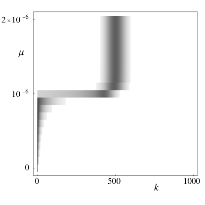
Figure 3: The stationary distribution, $\pi$, for the single-peaked landscape with $L=1000$ and $s=0.001$, as a function of the mutation rate per site, $\mu$. Types are lumped into classes: class $k$ contains all sequences with $\#_{1}(i)=k$, where $\#_{1}(i)$ is the number of 1’s in sequence $i$. Grey levels correspond to $\sum_{i:\#_{1}(i)=k}\pi_{k}$ (darker shading corresponds to larger values). The error threshold occurs at $\mu_{0}\approx s/L=10^{-6}$.

5 A two-type caricature.

To capture the essence of the single-peaked model, let us condense it radically. Assume that there are only two types, i.e., $S=\{0,1\}$, with birth rates $B_{0}=1+s$, $B_{1}=1$, death rates $D_{0}=D_{1}=1$, and mutation rates $U_{01}=u\nu_{1}$ and $U_{10}=u\nu_{0}$; cf. Fig. 4. Here, $u>0$ scales the overall mutation rate, whereas $\nu_{0}>0$ and $\nu_{1}>0$ ($\nu_{0}+\nu_{1}=1$) determine the asymmetry of mutation. To mimic the single-peaked model, with the fit sequence corresponding to type 0 and all others collected into type 1, a simple choice is $\nu_{0}=1/L$ and $u=\mu L$; it approximates the fact that, in the sequence picture, $\mu L$ is the total mutation rate away from $00\ldots 0$, and $\mu$ is the maximal rate at which an unfit individual can mutate back to the fit type. For this choice, $\pi$ and $\alpha$ are shown in Fig. 10 as a function of $u$. Unsurprisingly, the stationary frequency of the fit type decreases (almost linearly) with $u$, until it gets close to zero (around $u_{0}=s$). In contrast, the ancestral distribution consists almost exclusively of fit individuals until $u$ gets close to $u_{0}$, and then declines to zero quickly. (For $\nu_{0}\to 0$, the curves turn into piecewise linear ($\pi$) and piecewise constant ($\alpha$).) Obviously, for $u<u_{0}$, the present distribution carries with it a ‘comet tail’ of unfit mutants, which are present at any time, but do not survive in the long run. They therefore rarely show up as ancestors, nearly all of whom are fit.

Figure 4: The two-type mutation-reproduction process.

6 The Moran model with selection.

Branching processes have very nice features mathematically, because individuals reproduce independently of each other. Biologically, however, this independence can be quite unrealistic, because there is nothing to control population size. At the other extreme, one considers models for populations of fixed size. The standard models in this context are the Wright-Fisher model and the Moran model. We will use the Moran model here because, in contrast to the Wright-Fisher model, it has a continuous-time version, which leads to the coalescent in a most immediate way; furthermore, it readily compares to our branching process. Luckily, however, the choice is not essential, since both the Wright-Fisher and the Moran models share the same diffusion limit (up to a factor of 2, see Remark 2 below); and it is only in this limit that the model can be tackled explicitly anyway, as will become clear below.

Let us now embark on the counterpart of the two-type branching model of the previous Section, namely, the Moran model with two types, mutation and selection.

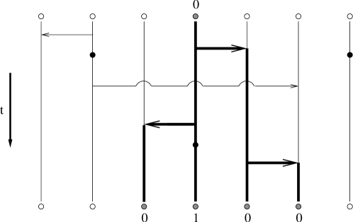
Figure 5: The Moran model. The fat lines represent the descendants of the single type-0 individual marked grey at the top ($t=0$). At the later time (bottom), its descendants consist of four individuals, one of whom has mutated to type 1 (mutation events are marked by blobs). Equivalently, the fat lines define the genealogy of the four ‘grey’ individuals at the bottom.

Moran models belong to the larger class of interacting particle systems, and are best explained in terms of their graphical representation, which, in our case, goes as follows (see Fig. 5). We have a fixed number of $N$ individuals, each characterised by a type $i\in S=\{0,1\}$, and represented by a vertical line; time runs from top to bottom. If an individual gives birth, the offspring inherits the parent’s type and replaces an individual chosen randomly from the population (maybe its own parent), thus keeping population size constant. In the graphical representation, such events are displayed as arrows, with the parent at the base and the offspring at the tip. Type-0 individuals reproduce at rate $1+s$, type-1 individuals at rate $1$. This type dependence of reproduction rates leads to selection, which means that, on average, unfit individuals are replaced by fit ones more often than vice versa, thus leading to a net replacement of unfit individuals by fit ones. Independently of reproduction, individuals may mutate, at rate $u\nu_{1}$ from type 0 to type 1, and at rate $u\nu_{0}$ in the reverse direction. Equivalently, we can say that every individual mutates at rate $u$, and the ensuing type is $i$ with probability $\nu_{i}$, $i\in S$; one thus includes some ‘empty events’ that, in effect, do not change the current type. Mutation events are represented as blobs in the graphical representation.

The graphical representation is not meant to encode any spatial information – all events are independent of the location of the individuals. Therefore, all relevant information is contained in the process $\{Y_{0}(t),Y_{1}(t)\}_{t\geq 0}$, where $Y_{i}(t)$, $i\in S$, is the number of individuals of type $i$ at time $t$ (of course, $Y_{0}(t)+Y_{1}(t)=N$, but we retain both components for convenience here). If the current state is $(Y_{0}(t),Y_{1}(t))=(k_{0},k_{1})$ ($k_{0}=0,\ldots,N$), the possible transitions are

$$(k_{0},k_{1})\to\begin{cases}(k_{0}+1,k_{1}-1)\;\text{at rate}\;u\nu_{0}k_{1}+(1+s)k_{0}k_{1}/N\\ (k_{0}-1,k_{1}+1)\;\text{at rate}\;u\nu_{1}k_{0}+k_{0}k_{1}/N\end{cases}$$

(note that transitions to ‘impossible’ states ($k_{i}\notin\{0,\ldots,N\}$) occur at rate zero and are therefore excluded).

The standard strategy to make the process tractable is to consider the normalised process $\{X_{0}(t),X_{1}(t)\}_{t\geq 0}:=\{Y_{0}(t),Y_{1}(t)\}_{t\geq 0}/N$, and take a diffusion limit, in which time is rescaled in units of $N$ generations, and the limit $N\to\infty$ is taken so that $Ns\to\sigma$ and $Nu\to\theta$, where $\theta>0$ and $\sigma\geq 0$. In this limit, the stationary distribution of type frequencies, in the forward direction of time, is well known: it is given by the density

(4) $$f(x_{0},x_{1})=\frac{1}{C}x_{0}^{\theta\nu_{0}-1}x_{1}^{\theta\nu_{1}-1}e^{\sigma x_{0}},$$

where $C$ is the normalising constant. Eq. (4) is a classical result known as Wright’s formula; see [11, Ch. 4,5] for a comprehensive review of diffusion theory in the context of population genetics.

In the diffusion limit, the above particle representation is no longer well-defined; a more advanced construction, known as the look-down process ([4, 5], see also [9, Ch. 5.2 and 5.3]) is required. In this tutorial introduction, we will only use the particle system for the finite population, and derive from it a good motivation for the backward construction in the diffusion limit.

Remark 1.  In most of the literature, the Moran model with selection is defined in a slightly different version, in which mutation events can only occur on the occasion of reproduction (see, e.g., [6, Chap. 3.1]). But this coupled version has the same diffusion limit as our parallel model, provided the parameters are interpreted in a suitable way; actually, one effect of the diffusion limit is to decouple mutation and selection, which are both rare events in the scaling chosen. We therefore prefer to start with the decoupled version right away.

Remark 2.  In the literature, a factor of 2 is often included in the mutation rates, selection intensities, and the time scale. The purpose of this is to make the Moran model comparable with the Wright-Fisher model, so that they share the same diffusion limit. More precisely, the factor of 2 comes from the fact that reproduction is tied to ordered pairs of individuals in the Moran model, but to unordered pairs in the Wright-Fisher model, cf. [6, p. 23]. Since we do not consider the Wright-Fisher model in this article, we will not stick to this convention, thus making our life easier. Let us note for completeness that a second factor of 2 may appear if populations are diploid (unlike the haploid populations considered here, they carry two copies of the genetic information per cell, which separate during reproduction, thus effectively duplicating the ‘population’ size).

7 Neutral genealogies.

The case without selection ($s=\sigma=0$), known as the neutral case in population genetics, is particularly simple. This is because reproduction rates do not depend on the type, and the reproduction and mutation processes may therefore be superimposed independently. This allows one to go beyond the ‘frequency picture’ considered in the previous Section, and also construct genealogies, i.e., answer the question: If I take a sample of $m$ individuals from a stationary population, which is the law that governs their joint history?

We will define a genealogy to consist of the genealogical tree and the types along the branches; the genealogical tree, in turn, is given by the tree topology together with the branch lengths (in units of time). If a realisation of the Moran model (in forward time) is given, the genealogy can be read off immediately by starting from the sampled individuals and tracing their ancestry backward (see Fig. 5): Every time the tip of an arrow is encountered, that arrow is followed backwards, and if it joins two lines in the genealogy, these lines merge. They thus give rise to a coalescence event, that is, two individuals go back to a common ancestor. The crucial point now is that realisations of genealogies can be constructed without constructing realisations of the forward process first, by a two-step procedure:

Start from our $m$ individuals and construct their genealogical tree, going backward in time and ignoring the types. To this end, recall that, in the graphical representation of the forward process, arrows appear at rate $1/N$ between any ordered pair of individuals (on the original time scale). Hence, arrows that lead to coalescence events appear at rate $1/N$ per ordered pair of lines in the genealogical tree. The number of lines currently in the tree is therefore a death process, which starts at $m$, decreases in unit steps at rate $n(n-1)/N$ if the current state is $n$, and ends in the absorbing state 1; at every death event, a random pair of lines is chosen to merge. The individual at the root of the tree is the most recent common ancestor (MRCA) of the sample. This verbal description defines the law, and an easy method of sampling, for genealogical trees. Rescaling of time turns the death rates into $n(n-1)$; the resulting stochastic process is known as the coalescent process, and goes back to Kingman [20, 21]. The types along the branches may then be determined in a second step, by picking the type of the most recent common ancestor from the stationary distribution (4) and running the mutation process forward in time along the genealogical tree (where, of course, both descendants inherit the parent’s type at a coalescence event).

8 The ancestral selection graph.

As mentioned above, the simplicity of the above construction relies on the fact that, in the neutral case, the mutation process may be superimposed independently onto the reproduction process, and hence the genealogical tree. But this independence breaks down as soon as there is selection. For this reason, the coalescent with selection has been considered intractable for more than a decade. Only within the last decade, Neuhauser and Krone [22, 23] and Donnelly and Kurtz [5] discovered constructions that overcome this problem. We will stick to the Neuhauser-Krone framework here, but the fundamental idea, in both constructions, is to again establish some kind of separation of the genealogical and the mutation processes. This is achieved by the following trick. Start with the forward particle system, and ignore the types. Decompose the original (type-dependent) reproduction process (before rescaling of time) into two independent processes, represented by two types of arrows: ‘neutral’ arrows that appear at rate 1 on every line regardless of the type (as in the neutral case, hence the name); and ‘selective’ arrows that appear at rate $s$, again on every line regardless of the type, but with the additional convention that the latter arrows are only ‘used’ if they emanate from a fit individual; otherwise, they are ignored. In contrast, neutral arrows are used in either case. Put differently, neutral arrows represent definitive birth events for everyone, whereas selective arrows correspond to potential birth events, to be used by fit individuals only. If we now reintroduce the types (by defining the initial types and adding in mutation events), the resulting process is equivalent to the original Moran model with selection (forward in time). Backward in time, it allows the construction of the genealogy of a sample taken from the stationary distribution, but now three steps are required, rather than two as in the neutral case. To explain the idea, let us give a verbal description, still starting from a given realisation of the collection of arrows in a finite particle system, but without knowledge of types; later, we will free ourselves from concrete realisations, and pass to the diffusion limit.

1. In a first step (see Fig. (A1), left panel), construct the so-called ancestral selection graph (ASG), without types. To this end, start from a sample of $m$ individuals from the present population, with the types unknown, and run time backward. This is done as follows. Given the realisation of the pattern of arrows, trace back the lines; every time you meet a neutral arrow, proceed in the familiar way, thus producing a coalescence event. However, if a selective arrow is encountered, there is a potential birth event which cannot be resolved yet since the types are still unknown. Depending on whether the arrow has or has not been used, there are two possible parents: the line at the base of the arrow (the incoming branch), or the line at the tip (the continuing branch). To keep track of both possibilities, the incoming branch is attached to the graph, which results in a branching event. (We ignore the possibility that the incoming branch may already be contained in the graph, since the probability for this vanishes in the diffusion limit.) The resulting branching-coalescing graph is known as the ASG (without types); all possible genealogical trees are embedded in it. When the number of lines reaches 1 for the first time, we have found the so-called ultimate ancestor (UA) of the population (not to be confused with the MRCA, see below). Note, however, that, going back further in time, the line emanating from the UA will, sooner or later, branch out again; the process may be continued indefinitely.

   Figure 6: Constructing the ASG. Left: Particle system with neutral arrows (solid) and selective arrows (dashed). Embedded (as bold lines) is the ASG without types, as obtained when going backward from the two ‘grey’ individuals sampled from the present population. Right: Starting from the UA, the mutation process is superimposed on the ASG, which may then be resolved into real (bold) and virtual (thin) branches according to Fig. (A2). The collection of bold lines (along with their types) constitutes the genealogy of the grey individuals.

   In the second step (see Fig. (A1), right panel), the type of the ultimate ancestor is drawn from the stationary distribution of the forward process. (It is not immediately obvious that the UA’s type should follow this distribution; the reason it does lies in the fact that the time when the ASG reaches size 1 is independent of the type, see the arguments in [26] and [5, Thm. 8.2]. Note that, even for finite $N$, the stationary distribution is available in closed form [28]; but it simplifies considerably in the diffusion limit.) Starting from the UA, the mutation process is then superimposed on the graph, running forward in time. As usual, both descendants inherit the parent’s type at a coalescence event. And now that the types are known, the branching events can be resolved as one goes along (see Fig. (A2)): If the incoming branch is fit, the selective birth event has indeed taken place, and the incoming branch is parental to the descendant individual (the one below the tip of the arrow); the continuing branch is called virtual. If the incoming branch is, however, unfit, then the birth event in question was fictitious, the incoming branch is virtual, and the continuing branch is the parental one. Note that, as a result, the descendant individual is unfit if and only if both the incoming and the continuing branches are unfit. The result of step (A2) is known as the ASG with types.

   Figure 7: Resolution of potential birth events. I incoming branch, C continuing branch, D descendant. The descendant line and its parental branch are marked bold.

   In the third and final step (see again Fig. (A1), right panel), the genealogy is extracted by moving backward in time once more. Starting at the sampled individuals, we trace their ancestry backwards along their parental lines identified in the previous step. The collection of all lines that are parental to the sampled individuals constitute the genealogical tree; they are also called real branches. All other lines are virtual (in particular, lines that are parental to virtual branches are themselves virtual), and are now removed from the picture to yield the genealogy. Note that the MRCA of the genealogical tree need not coincide with the UA of the ASG; it may be younger.

   The diffusion limit simplifies this construction in two respects. In (A1), the probability for the incoming branch to be one that is already within the ASG vanishes in the limit. And in (A2), it provides us with the simple explicit form of the stationary distribution (4) from which to pick the UA’s type. Forgetting about concrete realisations and considering that, after rescaling of time, selective arrows land on every line at rate $\sigma$, we can construct the ASG in the diffusive limit as the following analogue of (A1)–(A3):

   1. Construct the number of lines in the graph as a birth-death process, starting at $m$, with death rate $n(n-1)$ and birth rate $n\sigma$ when there are currently $n$ lines. From this, construct the ASG without types by choosing a random pair to coalesce at every death event, and choosing a random line to branch into two at every birth event. Stop when there is only one line left (this will almost surely happen in finite time [22, Thm. 3.2]).

   2. Pick the type of the ultimate ancestor from the stationary distribution (4). Run the mutation process down the graph (at rates $u\nu_{0}$ and $u\nu_{1}$) and resolve branching events as you go along, according to Fig. (A2).

   3. Extract the genealogy, as in (A3).

   An explicit algorithm is given in [26, Alg. 3.1].

   9 Tracing back single individuals.

   After describing the general idea of the ASG, we now turn to the simpler situation that arises if we trace back the ancestry of single individuals, picked from the stationary (present) distribution, rather than the genealogies of samples of several individuals. For this purpose, a simplified construction is available, which was recently presented by Fearnhead [12]. For a complementary approach, which relies on diffusion theory alone (without reference to genealogies), the reader is referred to Taylor [27]; we will restrict ourselves to the genealogical approach of [12] here. From now on, we will directly work with the diffusion limit.

   Even if only a single individual is sampled, its ancestral line will branch out at some stage; we will therefore still require the law for samples. Consider, therefore, a sample of size $m$ (which, for the moment, comes from the present population). One may either describe it as an ordered sample $\boldsymbol{c}=(c_{1},c_{2},\ldots,c_{m})$, where $c_{\ell}$ is the type of the $\ell$-th individual ($1\leq\ell\leq m$), or as an unordered sample $\boldsymbol{m}=(m_{0},m_{1})$, where $m_{i}$, $i\in S$, is the number of individuals of type $i$ (of course, $m_{0}+m_{1}=m$). Since there is no spatial information in our model, the law of our sample is invariant under permutations of the individuals. More precisely, if $p^{*}(\boldsymbol{c})$ is the probability of getting the ordered sample $\boldsymbol{c}$ when sampling $m$ individuals, we have $p^{*}(\hat{\boldsymbol{c}})=p^{*}(\boldsymbol{c})$ if $\#_{i}(\hat{\boldsymbol{c}})=\#_{i}(\boldsymbol{c})$, $i\in S$, where $\#_{i}(\boldsymbol{c})$ is the number of individuals of type $i$ in $\boldsymbol{c}$; this property is known as exchangeability in probability theory. One could therefore work with unordered samples; for our purpose, however, it is convenient (and compatible with [12]) to work with ordered samples, but to retain a slightly abusive notation reminiscent of unordered samples. Namely, we will denote by $p(\boldsymbol{m})$ the probability of any ordered sample that has $m_{0}$ 0-individuals and $m_{1}$ 1-individuals. More precisely, $p(\boldsymbol{m})$ satisfies $p^{*}(\boldsymbol{c})=p(\boldsymbol{m})$ for every $\boldsymbol{c}$ with $\#_{0}(\boldsymbol{c})=m_{0}$ and $\#_{1}(\boldsymbol{c})=m_{1}$. By Wright’s formula (4), we have $p(\boldsymbol{m})=\mathbb{E}(X_{0}^{m_{0}}X_{1}^{m_{1}})=\int_{\mathcal{X}}x_{0}^{m_{0}}x_{1}^{m_{1}}f(x_{0},x_{1})dx_{0}dx_{1}$, where $\mathcal{X}:=\{(x_{0},x_{1})\mid x_{0},x_{1}\geq 0\;\text{for}\;i\in S,x_{0}+x_{1}=1\}$. For later use, let us also define

   (5) $$p(j\mid\boldsymbol{m}):=\frac{p(\boldsymbol{m}+\boldsymbol{e}_{j})}{p(\boldsymbol{m})},\quad j\in S,$$

   where $\boldsymbol{e}_{0}:=(1,0)$ and $\boldsymbol{e}_{1}:=(0,1)$; in words, $p(j\mid\boldsymbol{m})$ is the probability of obtaining an individual of type $j$ if we have already drawn a sample $\boldsymbol{m}$ and pick one additional individual from the stationary distribution.

   Armed this way, let us now describe the construction of the ancestral line of a single individual. A further simplification will result from the fact that the types will be included throughout. Modifying the construction (A1’)–(A3’), one proceeds in the following way (see [12] and [26] for details):

   1. Pick an individual (i.e., a sample of size one) from the present population. Choose its type according to Wright’s formula (4), i.e., $p(\boldsymbol{e}_{i})=\mathbb{E}(X_{i})$, $i\in S$.

   2. Given this type, construct the ASG including the types. This only requires a single step because, given the initial type, the mutation process may be run backward, and, when a branching event is encountered, the type of the descendant is already known — and hence the type of the parental branch (be it ‘incoming’ or ‘continuing’), because it coincides with the type of the descendant. This way, potential birth events can be resolved on the way back already, thus contracting steps (A1’) and (A2’). In particular, this applies to the real branch (there is exactly one real branch throughout – the line parental to the single individual picked in step (B1)). What needs to be assigned at a branching event is the type of the virtual branch that appears; this can be done by using Fig. 8, and will be formalised below. Let us only conclude here that the ASG boils down to a process with states $(i;\boldsymbol{n})\in S\times\mathbb{Z}_{\geq 0}^{2}$, where $i$ denotes the type of the real branch, and $\boldsymbol{n}=(n_{0},n_{1})$ collects the numbers of virtual branches of type $0$ and $1$, respectively.

   Ultimately, to determine the ancestral distribution of types analogous to that of the branching process, we will only need the real branch – but to determine its type, the virtual ones are indispensable, as will become clear in a moment.

   10 Transitions and rates of the ASG, including the types.

   Let us now make precise step (B2) by recapitulating from [12] the definition of the ASG in terms of its transitions and the corresponding rates; for a detailed derivation, we refer the reader to [12] and [26, Alg. 3.2]. Let us only recall here that working backward in time (relative to the stationary measure $p$ of ordered samples) is analogous to constructing the generator for the time-reversed version of a continuous-time Markov chain on a state space $E$, as given by $\bar{Q}=(\bar{Q}_{ij})_{i,j\in E}$, where $\bar{Q}_{ij}=\pi_{i}^{-1}Q_{ji}\pi_{j}$ if $Q=(Q_{ij})_{i,j\in E}$ is the generator of the forward process and $\pi=(\pi_{i})_{i\in E}$ is the corresponding stationary distribution; cf. [24, Ch. 3.7] for some introductory material on time reversal; and compare the related time-reversed branching process in Sec. 2. Let us also note that, for ease of exposition, we will include ‘empty events’ in the context of mutation (as in Sec. 6).

   Given that the current state is $(i;\boldsymbol{n})$ and going backward in time, five types of events can occur (cf. Fig. 8); note that $(i;\boldsymbol{n})$ corresponds to a sample $\boldsymbol{n}+\boldsymbol{e}_{i}$.

   Figure 8: Transitions of the ASG, including the types. Transitions (C1)–(C5) out of $(i;\boldsymbol{n})$ in the ASG with types. The bold line is the real branch, the thin lines represent virtual branches. Blobs mark mutation events, crosses mark branches whose types are obtained as a random draw according to (5), and may be removed. In (C4), the continuing branch is parental; in (C5), the incoming branch is parental. Backward time runs from bottom to top.

   1. Mutation of the real branch: $(i;\boldsymbol{n})\to(j;\boldsymbol{n})$, $j\in S$, occurs at rate $\theta\nu_{i}p(\boldsymbol{n}+\boldsymbol{e}_{j})/p(\boldsymbol{n}+\boldsymbol{e}_{i})$, in accordance with the above reversion recipe.

   2. Mutation of a virtual branch: $(i;\boldsymbol{n})\to(i;\boldsymbol{n}+\boldsymbol{e}_{k}-\boldsymbol{e}_{j})$, $j,k\in S$, occurs at rate $n_{j}\theta\nu_{j}p(\boldsymbol{n}+\boldsymbol{e}_{i}-\boldsymbol{e}_{j}+\boldsymbol{e}_{k})/p(\boldsymbol{n}+\boldsymbol{e}_{i})$. The factor $n_{j}$ comes from the fact that, in the corresponding forward transition, $(i,\boldsymbol{n})$ is the target state and contains $n_{j}$ virtual branches of type $j$, each of which may have arisen by mutation (recall that $p(\boldsymbol{m})$ is the probability of any ordered sample of composition $\boldsymbol{m}$). Let us note for later use that, by (5), the rate may be rewritten as $(n_{j}\theta\nu_{j}p(\boldsymbol{n}+\boldsymbol{e}_{i}-\boldsymbol{e}_{j})/p(\boldsymbol{n}+\boldsymbol{e}_{i}))\times$ $p(k\mid\boldsymbol{n}+\boldsymbol{e}_{i}-\boldsymbol{e}_{j})$, that is, the type of the mutated branch can be obtained as a random draw from the stationary population, given the other branches in the sample.

   3. Coalescence of two branches of type $j$, $j\in S$: $(i;\boldsymbol{n})\to(i;\boldsymbol{n}-\boldsymbol{e}_{j})$ occurs at rate $(n_{j}+\delta_{ij})(n_{j}+\delta_{ij}-1)p(\boldsymbol{n}+\boldsymbol{e}_{i}-\boldsymbol{e}_{j})/p(\boldsymbol{n}+\boldsymbol{e}_{i})$. The combinatorial factor reflects the fact that coalescence events may involve both real and virtual branches, but can only occur between like types; for type $j$, there are $(n_{j}+\delta_{ij})(n_{j}+\delta_{ij}-1)$ ordered pairs of type $j$.

   4. Branching to an unfit incoming branch (see also Fig. (A2), (a) and (b)): $(i;\boldsymbol{n})\to(i;\boldsymbol{n}+\boldsymbol{e}_{1})$ occurs at rate $(n_{j}+\delta_{ij})\sigma p(\boldsymbol{n}+\boldsymbol{e}_{i}+\boldsymbol{e}_{1})/p(\boldsymbol{n}+\boldsymbol{e}_{i})$, for every $j\in S$. Here, the continuing branch (regardless of its type) is parental, and its type is thus the same as before the branching event.

   5. Branching to a fit incoming branch (see also Fig. (A2), (c) and (d)): $(i;\boldsymbol{n})\to(i;\boldsymbol{n}+\boldsymbol{e}_{k})$, $k\in S$, occurs at rate ($n_{0}+\delta_{i0})\sigma p(\boldsymbol{n}+\boldsymbol{e}_{i}+\boldsymbol{e}_{k})/p(\boldsymbol{n}+\boldsymbol{e}_{i})=(n_{0}+\delta_{i0})\sigma p(k\mid\boldsymbol{n}+\boldsymbol{e}_{i})$. Here, the incoming branch is parental; the type of the continuing branch may be obtained as a random draw conditional on the remaining sample, similar to the situation in (C2).

   The form of the mutation rate in (C1) is essential to understanding why we must keep track of the virtual branches at all, if we are, ultimately, only interested in the type of the real branch: the mutation process on the real branch depends on the full state of the process, including the virtual branches. Considering the real branch in isolation would, therefore, not lead to a Markov process. Indeed, the achievement of the ASG construction, and further simplifications like the common ancestor process below, lies just in the construction of a process with a state space that is ‘as small as possible’, with as few transitions as possible, while still retaining the Markov property. Indeed, the lines in the ASG only represent a vanishing proportion of the population (which is infinite in the diffusion limit!); loosely speaking, they may be considered a ‘representative sample’.

   11 The common ancestor process.

   Since we are only interested in the history of one individual, genealogical trees do not matter. This allows for a further simplification. According to [12, Thm. 1], virtual branches whose types have the law of a random draw from the stationary population (conditionally on the types of the remaining sample, as in events (C2) and (C5)) may be removed; the remaining ones still perform a Markov process defined by the events and rates (C1)–(C5). The intuition behind this is the following. Let $k$ be the type of a virtual branch in question, in a sample $(\boldsymbol{m}+\boldsymbol{e}_{k})$. If $k$ is distributed according to $p(k\mid\boldsymbol{m})$, then it contains no information about the history of the remaining sample, as suggested by the following thought experiment. Consider you draw $m+1$ individuals from the population, but determine only the type of $m$ of them, resulting in the (known) sample $\boldsymbol{m}$. Then $p(k\mid\boldsymbol{m})$ is the law of the type of the unknown individual. Clearly, then, the history of the known individuals is an ASG, regardless of the unknown type.

   Consider now events (C2) and (C5). Since, in both cases, the type of a virtual branch has a distribution of the form $p(k\mid\boldsymbol{m})$, it can safely be removed from the ASG without influencing the other branches (and, in particular, the history of the ancestor). Removal of the mutated virtual branch in (C2) turns this transition into one that is indistinguishable from a coalescence event of two virtual branches, (C3). Step (C5) may be removed altogether, since removal of the newly-created virtual branch turns the transition into an ‘empty’ one. As a consequence, virtual branches can now only arise due to (C4) and are all unfit. Therefore, $n_{0}=0$ throughout, and we set $n:=n_{1}$ in what follows. We thus arrive at what was termed the common ancestor process (CAP) in [12], and defined by its transitions out of $(i;\boldsymbol{n})$:

   1. Mutation of the real branch: $(i;\boldsymbol{n})\to(j;\boldsymbol{n})$, $j\in S$, at rate $\theta\nu_{i}p(\boldsymbol{n}+\boldsymbol{e}_{j})/p(\boldsymbol{n}+\boldsymbol{e}_{i})$;

   2. Removal of a virtual branch (by coalescence or mutation): $(i;\boldsymbol{n})\to(i;\boldsymbol{n}-\boldsymbol{e}_{1})$ at rate $[(n_{1}+\delta_{i1})(n_{1}+\delta_{i1}-1)+\theta\nu_{1}n_{1}]p(\boldsymbol{n}+\boldsymbol{e}_{i}-\boldsymbol{e}_{1})/p(\boldsymbol{n}+\boldsymbol{e}_{i})$;

   3. Branching: $(i;\boldsymbol{n})\to(i;\boldsymbol{n}+\boldsymbol{e}_{1})$ at rate $\sigma(n_{1}+1)p(\boldsymbol{n}+\boldsymbol{e}_{i}+\boldsymbol{e}_{j})/p(\boldsymbol{n}+\boldsymbol{e}_{i})$. (Note the typo in this rate in [12]: the factor $(n_{1}+1)$ is missing.)

   The process starts in state $(i;(0,0))$ with probability $p(\boldsymbol{e}_{i})$. A realisation is shown in Fig. 11. Note that the above notation of the states is somewhat redundant (the support of the process is $E=S\times\{0\}\times\mathbb{Z}_{\geq 0}$), but we retain it here for compatibility with the ‘full’ ASG.

   Figure 9: The common ancestor process. The solid line is the real branch, thin lines are virtual branches, numbers on lines mark their type. Backward time runs from bottom to top. Mutation events are marked by crosses; they lead to a change of type on the real branch, but to extinction on virtual branches. Virtual branches are all unfit. The state of the process between events is given to the right.

   12 The stationary distribution of the common ancestor process.

   By Thm. 3 and Lemma 1 of [12], the stationary distribution $a$ of the CAP is given by

   (6) $$a(i;\boldsymbol{n})=A_{n}(i)p(\boldsymbol{n}+\boldsymbol{e}_{i}),\quad(i;\boldsymbol{n})\in E,$$

   where $A_{n}(0):=\prod_{j=1}^{n}\lambda_{j}$, $A_{n}(1):=A_{n}(0)(1-\lambda_{n+1})$, and $\lambda_{j}:=\lim_{k\to\infty}\lambda_{j}^{(k)}$ ($j\geq 1$), where the $\lambda_{j}^{(k)}$ ($k\geq 0$) are defined by $\lambda_{k+1}^{(k)}=0$, together with the recursion

   (7) $$\lambda_{j-1}^{(k)}=\frac{\sigma}{j+\theta+\sigma-(j+\theta\nu_{1})\lambda_{j}^{(k)}}\,.$$

   The proof is by direct, though slightly cumbersome, verification; an alternate proof, which uses advanced diffusion theory rather than the ASG, is given in [27]. But a nice interpretation is also available [12], which turns (6) into the following rule for simulating from the distribution $a$ [12]. Choose an individual at random from the present distribution (4). If the individual is fit, call it the real branch (i.e., the ancestor). If the individual is unfit, then with probability $1-\lambda_{1}$ call it the ancestor; otherwise, call it a virtual branch, and pick another individual from the present distribution. Repeat this (i.e., if the $j$’th individual chosen is unfit, then with probability $1-\lambda_{j}$ it is the ancestor, otherwise draw another one) until you find the ancestor. When the ancestor has been found, the state $(i;\boldsymbol{n})$ is given by the type $i$ of the ancestor, and the number $n_{1}$ of virtual branches (and $n_{0}=0$).

   Marginalising over the virtual branches finally results in the stationary distribution of the ancestral type; more precisely, $a_{i}:=\sum_{n\geq 0}a(i;n)$ is the stationary probability that the ancestor has type $i$. Clearly, this is the desired analogue of $\alpha_{i}$ in the branching process.

   13 An example.

   Recall the two-type branching caricature of the single-peaked model (Sec. 5), and let us compare it to its Moran analogue. For the values of $s$ and $\nu_{0}$ used before, Fig. 10 shows the stationary frequencies of fit individuals in the present and ancestral population, as a function of $u$, and for various population sizes (that is, we take the approximating diffusion defined by the choice $\sigma=Ns$, $\theta=Nu$, for given $s$ and $u$). More precisely, the Figure depicts the expected frequency of fit individuals in the present population, $p(\boldsymbol{e}_{0})=\mathbb{E}(X_{0})$ as given by Wright’s formula; and the expected frequency of fit ancestors of individuals sampled randomly from the present population, as given by $a_{0}$. Comparing these with the corresponding stationary frequencies $\pi_{0}$ and $\alpha_{0}$ in the branching process suggests that the stationary distribution of the branching process is related to another $N\to\infty$ limit of the Moran model, which differs from the diffusion limit. Indeed, the Moran model (forward in time) also has a law of large numbers: Consider a sequence of Moran models with fixed $s$ and $u$, and increasing $N$, without rescaling of time. Denote the corresponding normalised processes by $\{X_{0}^{(N)}(t),X_{1}^{(N)}(t)\}_{t\geq 0}$, where the upper index is now introduced to denote dependence on population size. One can then show that, for $N\to\infty$, the sequence of generators of the processes $\{X_{0}^{(N)}(t),X_{1}^{(N)}(t)\}_{t\geq 0}$ converges, in a suitable sense, to the generator of the deterministic process defined by the system of ordinary differential equations

   (8) $$\dot{p}_{i}(t)=(R_{i}-\langle R,p\rangle)p_{i}(t)+\sum_{j:j\neq i}(p_{j}(t)U_{ji}-p_{i}(t)U_{ij}),\quad i\in S,$$

   where $p_{i}(t)$ is the relative frequency of type $i$ at time $t$ (details will be given elsewhere). By Thms. 1.6.1 and 4.9.10 of [10], this implies weak convergence of the stationary distributions of $\{X_{0}^{(N)}(t),X_{1}^{(N)}(t)\}_{t\geq 0}$ to the stationary distribution of (8). But the latter, in turn, is easily seen to coincide with the stationary distribution $\pi$ of the branching process (see, e.g., [3]). (A corresponding relationship for the backward process, suggestive as it may seem, remains to be formally established.)

   It is interesting to observe how the convergence of the stationary distribution manifests itself (see Fig. 10). The Moran curves follow the branching curves closely for small $u$ and then break off; this happens at values of $u$ that approach $u_{0}=s$ with increasing population size. Therefore, the branching result is an excellent approximation even for small and moderate-sized populations, as long as mutation rates are small.

   These observations complement previous studies [25, 28], which only considered the forward direction of time (they actually originated well before the ancestral selection graph). Let us note that the transition (in both branching and Moran models) becomes much steeper when the mutation rates are even more asymmetric than assumed here; the behaviour can then be interpreted as an error threshold for finite populations [28], but this is not our concern here.

   

   

   Figure 10: The present and ancestral frequencies of the fit type in the two-type branching process and the corresponding Moran model with selection, as a function of the mutation rate. Parameters: $s=0.001$, $\nu_{1}=0.999$. Left: Expected frequency of fit individuals in the stationary present distribution. Bold line: $\pi_{0}$, of the branching process; thin lines: $p(\boldsymbol{e}_{0})$ in the Moran model, for $N=10000$ (dotted), $N=30000$ (dashed), and $N=100000$ (solid line), according to Wright’s formula (4). Right: Expected frequency of fit individuals in the ancestral distribution. Bold line: $\alpha_{0}$, of the branching process; thin lines: $a_{0}$ in the Moran model, for $N=10000$ (dotted), $N=30000$ (dashed), and $N=100000$ (solid line). Here, $a_{0}$ is approximated by simulating according to the recipe resulting from (6), and averaging over 10000 realisations. The $\lambda_{j}$ required in the simulation are approximated by setting $\lambda_{500}^{(499)}=0$, and using the recursion (7).

   14 The virtual branches.

   The transition described above is intimately connected with the number of virtual branches – in fact, it is accompanied by an explosion of the expected number of virtual branches, see Fig. 11 (left panel). This can only be understood in the light of how the $\lambda_{j}$ depend on $u$. As shown in Fig. 11 (right panel), $\lambda_{1}$ is very close to 1 at $u=0$, and the $\lambda_{j}$ decrease with $u$, as well as $j$. The shape of the ancestral distribution may then be understood as follows. For $N=10000$, $s,\nu$ as in Fig. 10, and $u$ well below $0.0005$, simulation according to the ‘recipe’ resulting from (6) is similar to drawing from the present distribution until a fit individual is found, which is then identified as the ancestor — this is because $\lambda_{j}$ is close to 1 for $j\leq 100$; and the expected frequency of fit individuals in the present population, $p(\boldsymbol{e}_{0})$, is not too small, so that, typically, only few draws are required to find a fit individual. Therefore, the ancestors are almost all fit, although the present population is not — at the expense of an increasing number of virtuals. With increasing $u$ (and, correspondingly, decreasing $p(\boldsymbol{e}_{0})$), however, one needs more and more trials to find a fit individual; this leads to a further increase in the number of virtuals, increasing $j$ and decreasing $\lambda_{j}$. As a consequence, it becomes more and more likely to ‘accept’ an unfit individual as the ancestor; finally (beyond $u\sim 0.0005$), both the present and the ancestral population consist of mainly unfit individuals. But a large number of virtual branches is still present, because, for small $j$, the $\lambda_{j}$ are still close to one. The number of virtual branches only decreases slowly, in accordance with the decrease of the $\lambda_{j}$ with $u$.

   

   

   Figure 11: The virtual branches and how they originate. The situation corresponds to the dotted curve in Fig. 10, i.e., $N=10000$, $s=0.001$, $\nu_{1}=0.999$. Left panel: Expected number of virtual branches, as a function of the mutation rate. The number of virtual branches, $V$, is simulated as in Fig. 10 (right), and averaged over 10000 realisations to obtain an approximation of its expectation, $E(V)$. Right panel: The $\lambda_{j}$ as a function of the mutation rate, calculated as in Fig. 10 (right).

   15 Acknowledgement.

   It is our pleasure to thank Michael Baake, Paul Fearnhead, Steve Krone, and Jay Taylor for enlightening discussions and help with details, and Jay Taylor and John Wakeley for critically reading the manuscript. This work was supported by the Dutch-German Bilateral Research Group on Random Spatial Models in Physics and Biology (DFG-FOR 498).

References

- [1] K. B. Athreya and P. E. Ney, Branching Processes. Springer, New York, 1972.
- [2] E. Baake and W. Gabriel, Biological evolution through mutation, selection, and drift: an introductory review. In D. Stauffer (ed.), Ann. Rev. Comp. Phys., vol. 9, pp. 203–264, World Scientific, Singapore, 2000; arXiv:cond-mat/9907372.
- [3] E. Baake and H.-O. Georgii, Mutation, selection and ancestry in branching models: a variational approach. J. Math. Biol. 54 (2007), 257–303; arXiv:q-bio/0611018.
- [4] P. Donnelly and T. Kurtz, A countable representation of the Fleming-Viot measure-valued diffusion. Ann. Prob. 24 (1996), 698–742.
- [5] P. Donnelly and T. Kurtz, Genealogical processes for Fleming-Viot models with selection and recombination. Ann. Appl. Prob. 9 (1999), 1091–1148.
- [6] R. Durrett, Probability Models for DNA Sequence Evolution. Springer, New York, 2002.
- [7] M. Eigen, Selforganization of matter and the evolution of biological macromolecules. Naturwiss. 58 (1971), 465–523.
- [8] M. Eigen, J. McCaskill, and P. Schuster, The molecular quasi-species. Adv. Chem. Phys. 75 (1989), 149–263.
- [9] A. Etheridge. Introduction to Superprocesses. AMS, Providence, RI, 2000.
- [10] S. N. Ethier and T. G. Kurtz, Markov Processes – Characterization and Convergence. Wiley, New York, 1986; Reprint 2005.
- [11] W. Ewens. Mathematical Population Genetics. 2nd ed., Springer, Berlin, 2004.
- [12] P. Fearnhead, The common ancestor at a nonneutral locus. J. Appl. Prob. 39 (2002), 38–54.
- [13] H.-O. Georgii and E. Baake, Multitype branching processes: the ancestral types of typical individuals. Adv. Appl. Prob. 35 (2003), 1090–1110; arXiv:math/0302049.
- [14] J. Hermisson, O. Redner, H. Wagner, and E. Baake, Mutation-selection balance: Ancestry, load, and maximum principle. Theor. Pop. Biol. 62 (2002), 9–46; arXiv:cond-mat/0202432.
- [15] P. Jagers, General branching processes as Markov fields. Stoch. Proc. Appl. 32 (1989), 183–242.
- [16] P. Jagers, Stabilities and instabilities in population dynamics. J. Appl. Prob. 29 (1992), 770–780.
- [17] K. S. Karlin and H. M. Taylor, A first course in stochastic processes. 2nd ed., Academic Press, San Diego, CA, 1975.
- [18] J. G. Kemeny and J. L. Snell, Finite Markov Chains. Springer, New York, 1981.
- [19] H. Kesten and B. P. Stigum, A limit theorem for multidimensional Galton-Watson processes. Ann. Math. Statist. 37 (1966), 1211–1233.
- [20] J. F. C. Kingman, The coalescent. Stoch. Proc. Appl. 13 (1982), 235–248.
- [21] J. F. C. Kingman, On the genealogy of large populations. J. Appl. Prob. 19A (1982), 27–43.
- [22] S. Krone and C. Neuhauser, Ancestral processes with selection. Theor. Pop. Biol. 51 (1997), 210–237.
- [23] C. Neuhauser and S. Krone, The genealogy of samples in models with selection. Genetics 145 (1997), 519–534.
- [24] J. R. Norris, Markov Chains. Cambridge University Press, Cambridge, 1997 (reprint 1999).
- [25] M. Nowak and P. Schuster, Error thresholds of replication in finite populations: Mutation frequencies and the onset of Muller’s ratchet. J. Theor. Biol. 137 (1989), 375–395.
- [26] M. Stephens and P. Donnelly, Ancestral inference in population genetics models with selection. Austral. New Zeal. J. Stat. 51 (2003), 901–931.
- [27] J. E. Taylor, The common ancestor process for a Wright-Fisher diffusion, Electron. J. Probab. 12 (2007), 808–847.
- [28] T. Wiehe, E. Baake, and P. Schuster, Error propagation in reproduction of diploid organisms. J. Theor. Biol. 177 (1995), 1–15.
- (A2)